Enhanced Sliding Variable-Based Robust Adaptive Control for Canonical Nonlinear System with Unknown Dynamic and Control Gain

Abstract

This study presents an advanced Sliding Variable-Based Robust Adaptive Control (SVRAC) scheme designed for canonical nonlinear system with unknown dynamic and control gain functions. Leveraging neural network (NN) approximation, the proposed method simplifies control design by eliminating the need for traditional sliding mode control (SMC) components like equivalent and switching controls. SVRAC integrates three key elements: a feedback control term to stabilize system errors, a NN-based term to estimate and compensate for uncertainties, and a robustness adjustment term to maintain control integrity under dynamic variations. Theoretical validation through Lyapunov stability analysis confirms that the system errors are Semi-Globally Uniformly Ultimately Bounded (SGUUB), and the tracking error converges to a neighborhood of zero. Numerical and engineering simulations further demonstrate that SVRAC achieves superior tracking performance, robustness, and adaptability compared to conventional methods. This approach offers a streamlined yet effective solution for managing uncertainties in complex nonlinear systems, with potential applications across diverse engineering domains.

1. Introduction

Nonlinear systems in canonical form represent a class of systems that can be described in a standardized structure, simplifying the analysis and design of control strategies. Such systems frequently arise in engineering applications, including robotic manipulators [1], electrical power systems [2], and chemical processes [3], where precise modeling and control are critical. However, effectively controlling nonlinear systems in canonical form remains a challenging task, particularly in the presence of system uncertainties and dynamic variations.

Sliding mode control (SMC) is a robust control technique that has been extensively utilized in engineering applications, such as automotive systems, aerospace control, and robotics, owing to its resilience against parameter uncertainties and external disturbances [4]. SMC ensures desirable dynamic characteristics by driving the system states to a predefined sliding surface and maintaining them there [5,6]. Despite its advantages, traditional SMC often requires the computation of equivalent and switching controls. Designing the equivalent control involves accurately modeling system dynamics to derive a continuous control law that ensures the system state remains on the sliding surface, while switching control necessitates selecting appropriate gains to account for uncertainties and disturbances. These complexities limit the practicality of traditional SMC in real-world applications [7,8].

Adaptive control, another effective strategy, addresses uncertainties by dynamically tuning controller parameters based on observed errors. Neural network (NN) and fuzzy logic system (FLS) have been integrated into adaptive control to exploit their superior function approximation capabilities, particularly for systems with unknown or uncertain dynamics [9,10,11,12]. While adaptive control methods have demonstrated success in various fields, such as autonomous vehicles and aerospace systems, they often rely on error-based adaptation mechanisms, which can lead to slow convergence and reduced robustness in highly dynamic environments [13,14].

To overcome the limitations of traditional SMC and adaptive control, Sliding Variable-Based Adaptive Control (SVAC) has been introduced, utilizing sliding variable instead of system error variables for adaptation. This approach offers significant advantages, including simplified controller design and enhanced robustness. However, when internal system uncertainties are substantial, the performance of SVAC can degrade. To address this, Sliding Variable-Based Robust Adaptive Control (SVRAC) introduces an additional robustness adjustment term, combining the strengths of SMC, adaptive control, and robust control theories [15,16].

In this study, we propose an enhanced SVRAC framework for canonical nonlinear system with unknown dynamic and control gain functions. The key contributions of this work are as follows:

(1)

To improve existing adaptive control methods based on NN and FLS, a robust adaptive control scheme is designed, incorporating feedback, NN-based uncertainty compensation, and robustness adjustment terms to improve tracking performance and stability.

(2)

The proposed method simplifies controller design by eliminating the need for equivalent and switching controls in traditional SMC.

(3)

Lyapunov stability analysis demonstrates the Semi-Globally Uniformly Ultimately Bounded (SGUUB) behavior of error variables and the convergence of the tracking error to a small neighborhood of zero.

(4)

Comprehensive numerical and engineering simulations validate the effectiveness of the proposed SVRAC approach, highlighting its adaptability and robustness under varying conditions.

By integrating advanced control strategies and NN-based approximation, the proposed SVRAC framework offers a practical and efficient solution for managing uncertainties in nonlinear systems, paving the way for broader applications in modern engineering systems.

2. System Statement and Preliminaries

This section introduces the canonical nonlinear system under consideration and outlines its mathematical formulation. Key assumptions about the system’s properties, such as bounded reference trajectories and consistent control gain signs, are stated to facilitate the subsequent control design. This section also discusses the role of the neural network (NN) in approximating unknown functions, leveraging its universal approximation capability to address uncertainties effectively.

2.1. System Formulation

Consider the following nonlinear system expressed in canonical dynamic form:

$$\begin{array}{cc}\hfill {\dot{\varpi }}_1\left(t\right)& ={\varpi }_2\left(t\right),\hfill \\ \hfill {\dot{\varpi }}_2\left(t\right)& ={\varpi }_3\left(t\right),\hfill \\ \hfill \cdots \\ \hfill {\dot{\varpi }}_n\left(t\right)& =f\left(\overline{\varpi }\right)+g\left(\overline{\varpi }\right)u,\hfill \end{array}$$

(1)

where $\overline{\varpi }\left(t\right)={[{\varpi }_1\left(t\right),{\varpi }_2\left(t\right),\cdots ,{\varpi }_n\left(t\right)]}^T\in {\mathbb{R}}^n$ represents the system state vector, ${\varpi }_1\left(t\right)\in \mathbb{R}$ represents the system output, $u\in \mathbb{R}$ represents the system input, $f\left(\overline{\varpi }\right)\in \mathbb{R}$ indicates an unknown continuous nonlinear dynamic function, and $g\left(\overline{\varpi }\right)\in \mathbb{R}$ indicates an unknown continuous control gain function.

Control objectives. Utilizing NN approximation, we develop a SVRAC framework tailored for the canonical nonlinear system characterized by unknown dynamic and control gain functions. This design should achieve the following objectives:

(1)

Ensure that all error variables within the closed-loop system exhibit Semi-Globally Uniformly Ultimately Bounded (SGUUB) behavior;

(2)

Enhance the system output ${\varpi }_1\left(t\right)$ to closely align with the reference signal ${\varpi }_r\left(t\right)$.

Assumption 1

([17]). The reference ${\varpi }_r\left(t\right)$ and its derivatives ${\dot{\varpi }}_r\left(t\right)$, ${\ddot{\varpi }}_r\left(t\right)$, ⋯, ${\varpi }_r^{\left(n\right)}\left(t\right)$ are continuous and bounded.

Assumption 2

([18]). The sign of $g\left(\overline{\varpi }\right)$ remains unchanged, and without loss of generality, we assume it is strictly positive. Furthermore, there exist two known positive constants, ${\eta }_1$ and ${\eta }_2$, such that ${\eta }_1\le g\left(\overline{\varpi }\right)\le {\eta }_2$.

Lemma 1

([19]). For a continuous positive function $Q\left(t\right)\in \mathbb{R}$, if it satisfies the inequality $\dot{Q}\left(t\right)\le -{\alpha }_{1}Q\left(t\right)+{\alpha }_2$, where ${\alpha }_1$ and ${\alpha }_2$ are positive constants, then the inequality below is satisfied:

$$\begin{array}{c}\hfill Q\left(t\right)\le e^{-{\alpha }_{1}t}Q\left(0\right)+{\displaystyle \frac{{\alpha }_2}{{\alpha }_1}}(1-e^{-{\alpha }_{1}t}).\end{array}$$

(2)

2.2. Neural Network

NN has a remarkable ability to approximate an unknown continuous function, thanks to its superior function approximation capability. For an unknown continuous function $\beth \left(\nu \right)$: ${\mathbb{R}}^n\to {\mathbb{R}}^m$ defined on a compact set ${\Omega }_{\nu }\in {\mathbb{R}}^n$, its NN approximation can be expressed as

$$\begin{array}{c}\hfill \widehat{\beth }\left(\nu \right)=V^{T}O\left(\nu \right),\end{array}$$

(3)

where $V\in {\mathbb{R}}^{s\times m}$ is the weight matrix, and s represents the number of neurons. Each element $O_i\left(\nu \right),i=1,\cdots s$ of the Gaussian basis function vector $O\left(\nu \right)={[O_1\left(\nu \right),\cdots ,O_s\left(\nu \right)]}^T$, corresponding to the input vector $\nu \in {\Omega }_{\nu }$, is defined as $O_i\left(\nu \right)=exp\left(-{\displaystyle \frac{{(\nu -{\psi }_i)}^T(\nu -{\psi }_i)}{{\tau }_i^2}}\right),$ where ${\tau }_i$ and ${\psi }_i={[{\psi }_{i1},{\psi }_{i2},\cdots ,{\psi }_{in}]}^T\in {\mathbb{R}}^n$ represent the width and the center vector of the Gaussian function, respectively. Moreover, there exists an ideal NN weight $V^{*}$, defined as $V^{*}\triangleq \underset{V\in {\mathbb{R}}^{s\times m}}{\arg \min }\left\{\underset{\nu \in {\Omega }_{\nu }}{\sup }\parallel \beth \left(\nu \right)-V^{T}O\left(\nu \right)\parallel \right\}$. Using this ideal weight, the function $\beth \left(\nu \right)$ can be approximated as

$$\begin{array}{c}\hfill \beth \left(\nu \right)=V^{*T}O\left(\nu \right)+\epsilon \left(\nu \right),\end{array}$$

(4)

where $\epsilon \left(\nu \right)\in {\mathbb{R}}^m$ represents the bounded approximation error [20].

3. Main Results

The proposed Sliding Variable-Based Robust Adaptive Control (SVRAC) framework is detailed in this section. It includes feedback control for stabilization, NN-based uncertainty compensation, and robustness adjustment for resilience. Lyapunov stability analysis proves that the system achieves bounded error behavior and tracks the desired trajectories with minimal error.

3.1. SVRAC Design

The tracking errors are defined as follows:

$$\begin{array}{cc}\hfill \beta \left(t\right)& ={\varpi }_1\left(t\right)-{\varpi }_r\left(t\right),\hfill \\ \hfill \dot{\beta }\left(t\right)& ={\varpi }_2\left(t\right)-{\dot{\varpi }}_r\left(t\right),\hfill \\ \hfill & \cdots \hfill \\ \hfill {\beta }^{(n-2)}\left(t\right)& ={\varpi }_{n-1}\left(t\right)-{\varpi }_r^{(n-2)}\left(t\right),\hfill \\ \hfill {\beta }^{(n-1)}\left(t\right)& ={\varpi }_n\left(t\right)-{\varpi }_r^{(n-1)}\left(t\right),\hfill \end{array}$$

(5)

Subsequently, the sliding variable is formulated as

$$\begin{array}{cc}\hfill \rho \left(t\right)& =c_1\beta \left(t\right)+c_2\dot{\beta }\left(t\right)+\cdots +c_{n-1}{\beta }^{(n-2)}\left(t\right)+{\beta }^{(n-1)}\left(t\right),\hfill \end{array}$$

(6)

where the constants $c_1,c_2,\cdots ,c_{n-1}$ are chosen to satisfy the Hurwitz polynomial $h\left(\lambda \right)=c_1+c_2\lambda +\cdots +c_{n-1}{\lambda }^{n-2}+{\lambda }^{n-1}$. This ensures that all the roots of the polynomial are located in the left half-plane, where $\lambda$ denotes the Laplace operator [21,22].

Based on (1) and the fact that ${\beta }^{\left(n\right)}={\dot{\varpi }}_n\left(t\right)-{\varpi }_r^{\left(n\right)}\left(t\right)$, we can derive the following expression:

$$\begin{array}{cc}\hfill \dot{\rho }\left(t\right)& =c_1\dot{\beta }\left(t\right)+c_2\ddot{\beta }\left(t\right)+\cdots +c_{n-1}{\beta }^{(n-1)}\left(t\right)+f\left(\overline{\varpi }\right)+g\left(\overline{\varpi }\right)u-{\varpi }_r^{\left(n\right)}\left(t\right)\hfill \\ \hfill & =F\left(\overline{\varpi }\right)+g\left(\overline{\varpi }\right)u-M\left({\varpi }_r\right),\hfill \end{array}$$

(7)

where $F\left(\overline{\varpi }\right)=c_1{\varpi }_2\left(t\right)+c_2{\varpi }_3\left(t\right)+\cdots +c_{n-1}{\varpi }_n\left(t\right)+f\left(\overline{\varpi }\right)$, and $M\left({\varpi }_r\right)=c_1{\dot{\varpi }}_r\left(t\right)+c_2{\ddot{\varpi }}_r\left(t\right)+\cdots +c_{n-1}{\varpi }_r^{(n-1)}\left(t\right)+{\varpi }_r^{\left(n\right)}\left(t\right)$ is bounded according to Assumption 1.

Define $L\left(\overline{\varpi }\right)=g{\left(\overline{\varpi }\right)}^{-1}F\left(\overline{\varpi }\right)\in \mathbb{R}$; then, (7) will become

$$\begin{array}{c}\hfill \dot{\rho }\left(t\right)=g\left(\overline{\varpi }\right)L\left(\overline{\varpi }\right)+g\left(\overline{\varpi }\right)u-M\left({\varpi }_r\right),\end{array}$$

(8)

It should be noted that the function $L\left(\overline{\varpi }\right)$ is unknown but continuous. To address this, the NN is implemented to approximate it over the given compact $\Omega$ using the following equation:

$$\begin{array}{c}\hfill L\left(\overline{\varpi }\right)=V_L^{*T}O\left(\overline{\varpi }\right)+\epsilon \left(\overline{\varpi }\right),\end{array}$$

(9)

where $V_L^{*}\in {\mathbb{R}}^p$ denotes the ideal NN weight, $O\left(\overline{\varpi }\right)\in {\mathbb{R}}^p$ denotes the basis function vector, and $\epsilon \left(\overline{\varpi }\right)\in \mathbb{R}$ represents the approximation error.

To obtain the actual control, the unknown weight $V_L^{*}$ needs to be estimated using the following adaptive training mechanism:

$$\begin{array}{c}\hfill \widehat{L}\left(\overline{\varpi }\right)={\widehat{V}}_L^T\left(t\right)O\left(\overline{\varpi }\right),\end{array}$$

(10)

where $\widehat{L}\left(\overline{\varpi }\right)\in \mathbb{R}$ is the estimated output, and ${\widehat{V}}_L\left(t\right)\in {\mathbb{R}}^p$ is the estimated weight.

Then, the SVRAC is formulated as follows:

$$u=\stackrel{SVRAC}{\overbrace{\underset{SVAC}{\underbrace{\underset{\begin{array}{c}\mathit{feedback}\\ \mathit{control}\end{array}}{\underbrace{-{\sigma }_1\rho \left(t\right)}}-\underset{\begin{array}{c}\mathit{NN}\\ \mathit{approximation}\end{array}}{\underbrace{{\widehat{V}}_L^T\left(t\right)O\left(\varpi \right)}}}}\underset{\begin{array}{c}\mathit{robustness}\\ \mathit{adjustment}\end{array}}{\underbrace{-{\sigma }_2\mathrm{sgn}\left(\rho \right)}}}},$$

(11)

where ${\sigma }_1>{\displaystyle \frac{{\eta }_2^2}{{\eta }_1}}+{\displaystyle \frac{1}{2{\eta }_1}}$ is a positive control gain constant [23], ${\sigma }_2$ is a designed positive constant, and the sign function sgn(·) is defined as

$$\begin{array}{c}\hfill \mathrm{sgn}(·)=\left\{\begin{array}{c}\begin{array}{cc}1& \mathrm{if}·>0,\hfill \\ 0& \mathrm{if}·=0,\hfill \\ -1& \mathrm{if}·<0.\hfill \end{array}\hfill \end{array}\right.\end{array}$$

Remark 1.

Unlike the SVAC presented in [15,16], the proposed SVRAC consists of three main components. The first component is the feedback control term, which stabilizes the system by responding to the error between the desired and actual states. The second component is the NN approximation term, which compensates for the unknown dynamic and uncertainties in the system by leveraging the NN’s ability to estimate unmodeled dynamic. The third component is the robustness adjustment term, which ensures that the control system remains stable and robust, even in the presence of estimation errors [24].

The adaptive law for tuning weight ${\widehat{V}}_L\left(t\right)$ is formulated as

$$\begin{array}{c}\hfill {\dot{\widehat{V}}}_L\left(t\right)=-{\gamma }_1\left(O\left(\overline{\varpi }\right)O^T\left(\overline{\varpi }\right){\widehat{V}}_L\left(t\right)+{\gamma }_2{\widehat{V}}_L\left(t\right)\right),\end{array}$$

(12)

where ${\gamma }_1$ and ${\gamma }_2$ are positive designed constants.

3.2. Theorem with Proof

Theorem 1.

Consider the canonical nonlinear system described by (1). If the actual control law (11) is implemented alongside the adaptive law (12), and the designed constants satisfy the required conditions, then the following objectives can be achieved:

(1) 

All error signals in the closed-loop system will be SGUUB;

(2) 

The system output will be able to closely follow the reference signal.

Proof. 

Choose the Lyapunov function as follows:

$$\begin{array}{c}\hfill Q\left(t\right)={\displaystyle \frac{1}{2}}{\rho }^2\left(t\right)+{\displaystyle \frac{1}{2}}{\gamma }_1{\tilde{V}}_L^T\left(t\right){\tilde{V}}_L\left(t\right),\end{array}$$

(13)

where ${\tilde{V}}_L\left(t\right)={\widehat{V}}_L\left(t\right)-V_L^{*}$ represents the weight approximation error.

The time derivative of $Q\left(t\right)$, based on (8) and (12), is expressed as follows:

$$\begin{array}{cc}\hfill \dot{Q}\left(t\right)=& \rho \left(t\right)\left(g\left(\overline{\varpi }\right)\left(L\left(\overline{\varpi }\right)+u\right)-M\left({\varpi }_r\right)\right)-{\tilde{V}}_L^T\left(t\right)\left(O\left(\overline{\varpi }\right)O^T\left(\overline{\varpi }\right){\widehat{V}}_L\left(t\right)+{\gamma }_2{\widehat{V}}_L\left(t\right)\right)\hfill \\ \hfill =& \rho \left(t\right)\left(g\left(\overline{\varpi }\right)\left(-{\sigma }_1\rho \left(t\right)-{\tilde{V}}_L^T\left(t\right)O\left(\overline{\varpi }\right)-{\sigma }_2\mathrm{sgn}\left(\rho \right)+\epsilon \left(\overline{\varpi }\right)\right)-M\left({\varpi }_r\right)\right)\hfill \\ \hfill & -{\tilde{V}}_L^T\left(t\right)\left(O\left(\overline{\varpi }\right)O^T\left(\overline{\varpi }\right){\widehat{V}}_L\left(t\right)+{\gamma }_2{\widehat{V}}_L\left(t\right)\right).\hfill \end{array}$$

(14)

Utilizing Young’s inequality [${\tau }_1{\tau }_2\le {\displaystyle \frac{{\tau }_1^2}{2}}+{\displaystyle \frac{{\tau }_2^2}{2}}$], we can derive the following results [25]:

$$\begin{array}{cc}\hfill -\rho \left(t\right)g\left(\overline{\varpi }\right){\tilde{V}}_L^T\left(t\right)O\left(\overline{\varpi }\right)& \le {\displaystyle \frac{{\eta }_2^2}{2}}{\rho }^2\left(t\right)+{\displaystyle \frac{1}{2}}{\tilde{V}}_L^T\left(t\right)O\left(\overline{\varpi }\right)O^T\left(\overline{\varpi }\right){\tilde{V}}_L\left(t\right),\hfill \\ \hfill \rho \left(t\right)g\left(\overline{\varpi }\right)\epsilon \left(\overline{\varpi }\right)& \le {\displaystyle \frac{{\eta }_2^2}{2}}{\rho }^2\left(t\right)+{\displaystyle \frac{1}{2}}{\epsilon }^2\left(\overline{\varpi }\right),\hfill \\ \hfill -\rho \left(t\right)M\left({\varpi }_r\right)& \le {\displaystyle \frac{1}{2}}{\rho }^2\left(t\right)+{\displaystyle \frac{1}{2}}{M}^2\left({\varpi }_r\right),\hfill \end{array}$$

(15)

Inserting (15) into (14) yields

$$\begin{array}{cc}\hfill \dot{Q}\left(t\right)\le & -({\eta }_1{\sigma }_1-{\eta }_2^2-{\displaystyle \frac{1}{2}}){\rho }^2\left(t\right)+{\displaystyle \frac{1}{2}}{\tilde{V}}_L^T\left(t\right)O\left(\overline{\varpi }\right)O^T\left(\overline{\varpi }\right){\tilde{V}}_L\left(t\right)\hfill \\ \hfill & -{\tilde{V}}_L^T\left(t\right)O\left(\overline{\varpi }\right)O^T\left(\overline{\varpi }\right){\widehat{V}}_L\left(t\right)-{\gamma }_2{\tilde{V}}_L^T\left(t\right){\widehat{V}}_L\left(t\right)+{\displaystyle \frac{1}{2}}{\epsilon }^2\left(\overline{\varpi }\right)+{\displaystyle \frac{1}{2}}{M}^2\left({\varpi }_r\right).\hfill \end{array}$$

(16)

According to ${\tilde{V}}_L\left(t\right)={\widehat{V}}_L\left(t\right)-V_L^{*}$, we can obtain

$$\begin{array}{cc}\hfill -{\tilde{V}}_L^T\left(t\right)O\left(\overline{\varpi }\right)O^T\left(\overline{\varpi }\right){\widehat{V}}_L\left(t\right)=& -{\displaystyle \frac{1}{2}}{\tilde{V}}_L^T\left(t\right)O\left(\overline{\varpi }\right)O^T\left(\overline{\varpi }\right){\tilde{V}}_L\left(t\right)-{\displaystyle \frac{1}{2}}{\widehat{V}}_L^T\left(t\right)O\left(\overline{\varpi }\right)O^T\left(\overline{\varpi }\right){\widehat{V}}_L\left(t\right)\hfill \\ \hfill & +{\displaystyle \frac{1}{2}}{V}_L^{*}O\left(\overline{\varpi }\right)O^T\left(\overline{\varpi }\right)V_L^{*},\hfill \end{array}$$

(17)

$$\begin{array}{cc}\hfill -{\gamma }_2{\tilde{V}}_L^T\left(t\right){\widehat{V}}_L\left(t\right)=& -{\displaystyle \frac{{\gamma }_2}{2}}{\tilde{V}}_L^T\left(t\right){\tilde{V}}_L\left(t\right)-{\displaystyle \frac{{\gamma }_2}{2}}{\widehat{V}}_L^T\left(t\right){\widehat{V}}_L\left(t\right)+{\displaystyle \frac{{\gamma }_2}{2}}{V}_L^{*T}{V}_L^{*}.\hfill \end{array}$$

(18)

Inserting (17) and (18) into (16) results in

$$\begin{array}{cc}\hfill \dot{Q}\left(t\right)\le & -({\eta }_1{\sigma }_1-{\eta }_2^2-{\displaystyle \frac{1}{2}}){\rho }^2\left(t\right)-{\displaystyle \frac{{\gamma }_2}{2}}{\tilde{V}}_L^T\left(t\right){\tilde{V}}_L\left(t\right)-{\displaystyle \frac{1}{2}}{\widehat{V}}_L^T\left(t\right)O\left(\overline{\varpi }\right)O^T\left(\overline{\varpi }\right){\widehat{V}}_L\left(t\right)\hfill \\ \hfill & -{\displaystyle \frac{{\gamma }_2}{2}}{\widehat{V}}_L^T\left(t\right){\widehat{V}}_L\left(t\right)+{\displaystyle \frac{1}{2}}{V}_L^{*}O\left(\overline{\varpi }\right)O^T\left(\overline{\varpi }\right)V_L^{*}+{\displaystyle \frac{{\gamma }_2}{2}}{V}_L^{*T}{V}_L^{*}+{\displaystyle \frac{1}{2}}{\epsilon }^2\left(\overline{\varpi }\right)+{\displaystyle \frac{1}{2}}{M}^2\left({\varpi }_r\right)\hfill \\ \hfill \le & -({\eta }_1{\sigma }_1-{\eta }_2^2-{\displaystyle \frac{1}{2}}){\rho }^2\left(t\right)-{\displaystyle \frac{{\gamma }_2}{2}}{\tilde{V}}_L^T\left(t\right){\tilde{V}}_L\left(t\right)+\Pi \left(t\right),\hfill \end{array}$$

(19)

where $\Pi \left(t\right)={\displaystyle \frac{1}{2}}{V}_L^{*}O\left(\overline{\varpi }\right)O^T\left(\overline{\varpi }\right)V_L^{*}+{\displaystyle \frac{{\gamma }_2}{2}}{V}_L^{*T}{V}_L^{*}+{\displaystyle \frac{1}{2}}{\epsilon }^2\left(\overline{\varpi }\right)+{\displaystyle \frac{1}{2}}{M}^2\left({\varpi }_r\right)$ and ${\alpha }_2=\underset{t\ge 0}{sup}\{\Pi \left(t\right)\}$.

Furthermore, the inequality (19) can be rewritten as

$$\begin{array}{cc}\hfill \dot{Q}\left(t\right)& \le -({\eta }_1{\sigma }_1-{\eta }_2^2-{\displaystyle \frac{1}{2}}){\rho }^2\left(t\right)-{\displaystyle \frac{{\gamma }_2}{2{\gamma }_1}}{\gamma }_1{\tilde{V}}_L^T\left(t\right){\tilde{V}}_L\left(t\right)+{\alpha }_2.\hfill \end{array}$$

(20)

If we let ${\alpha }_1=\min \{2\left({\eta }_1{\sigma }_1-{\eta }_2^2-{\displaystyle \frac{1}{2}}\right),{\displaystyle \frac{{\gamma }_2}{{\gamma }_1}}\}$, the inequality (20) can be expressed as

$$\begin{array}{cc}\hfill \dot{Q}\left(t\right)& \le -{\alpha }_{1}Q\left(t\right)+{\alpha }_2,\hfill \end{array}$$

(21)

To ensure that ${\alpha }_1$ is positive, as required by Lemma 1, we must satisfy the following condition:

$$\begin{array}{c}\hfill {\eta }_1{\sigma }_1-{\eta }_2^2-{\displaystyle \frac{1}{2}}>0\Rightarrow {\sigma }_1>{\displaystyle \frac{{\eta }_2^2}{{\eta }_1}}+{\displaystyle \frac{1}{2{\eta }_1}},\end{array}$$

(22)

It is evident that the requirement here aligns with the range of the control gain constant designed in (11).

Furthermore, by applying Lemma 1 to (21), we can obtain

$$\begin{array}{c}\hfill 0\le Q\left(t\right)\le e^{-{\alpha }_{1}t}Q\left(0\right)+{\displaystyle \frac{{\alpha }_2}{{\alpha }_1}}(1-e^{-{\alpha }_{1}t}),\end{array}$$

(23)

By incorporating the fact that ${lim}_{t\to \infty }\left(e^{-{\alpha }_{1}t}Q\left(0\right)+{\displaystyle \frac{{\alpha }_2}{{\alpha }_1}}(1-e^{-{\alpha }_{1}t})\right)={\displaystyle \frac{{\alpha }_2}{{\alpha }_1}}$, we can further derive

$$\begin{array}{c}\hfill \underset{t\to \infty }{lim}Q\left(t\right)\le {\displaystyle \frac{{\alpha }_2}{{\alpha }_1}}.\end{array}$$

(24)

The inequality (24) demonstrates that, regardless of the initial condition $Q\left(0\right)$, after a sufficiently long duration T, the function $Q\left(t\right)$ will be eventually governed by the term ${\displaystyle \frac{{\alpha }_2}{{\alpha }_1}}$ [26]. Specifically, there exists a time $T>0$ such that for all $t\ge T$, the Lyapunov function $Q\left(t\right)$ will remain within the compact set $\Omega =[0,{\displaystyle \frac{{\alpha }_2}{{\alpha }_1}}]$. It is evident that this satisfies the definition of SGUUB [27]. As a result, all closed-loop error signals, $\rho \left(t\right)$ and ${\tilde{V}}_L\left(t\right)$, are SGUUB. Moreover, by selecting a sufficiently large gain ${\sigma }_1$ in actual control (11), we can guarantee that the tracking error $\beta \left(t\right)$ converges to a small neighborhood around zero. □

4. Simulation Examples

This section demonstrates the SVRAC framework through numerical and engineering simulations, including a numerical nonlinear system and a rigid manipulator.

4.1. Example 1 (Numerical Example)

Consider the following third-order nonlinear system for numerical analysis:

$$\begin{array}{cc}\hfill {\dot{\varpi }}_1\left(t\right)& ={\varpi }_2\left(t\right),\hfill \\ \hfill {\dot{\varpi }}_2\left(t\right)& ={\varpi }_3\left(t\right),\hfill \\ \hfill {\dot{\varpi }}_3\left(t\right)& =sin\left({\varpi }_1\right)+0.2{\varpi }_2\left(t\right)cos\left({\varpi }_3\right)+1.3cos\left({\varpi }_1{\varpi }_2{\varpi }_3\right)u,\hfill \end{array}$$

(25)

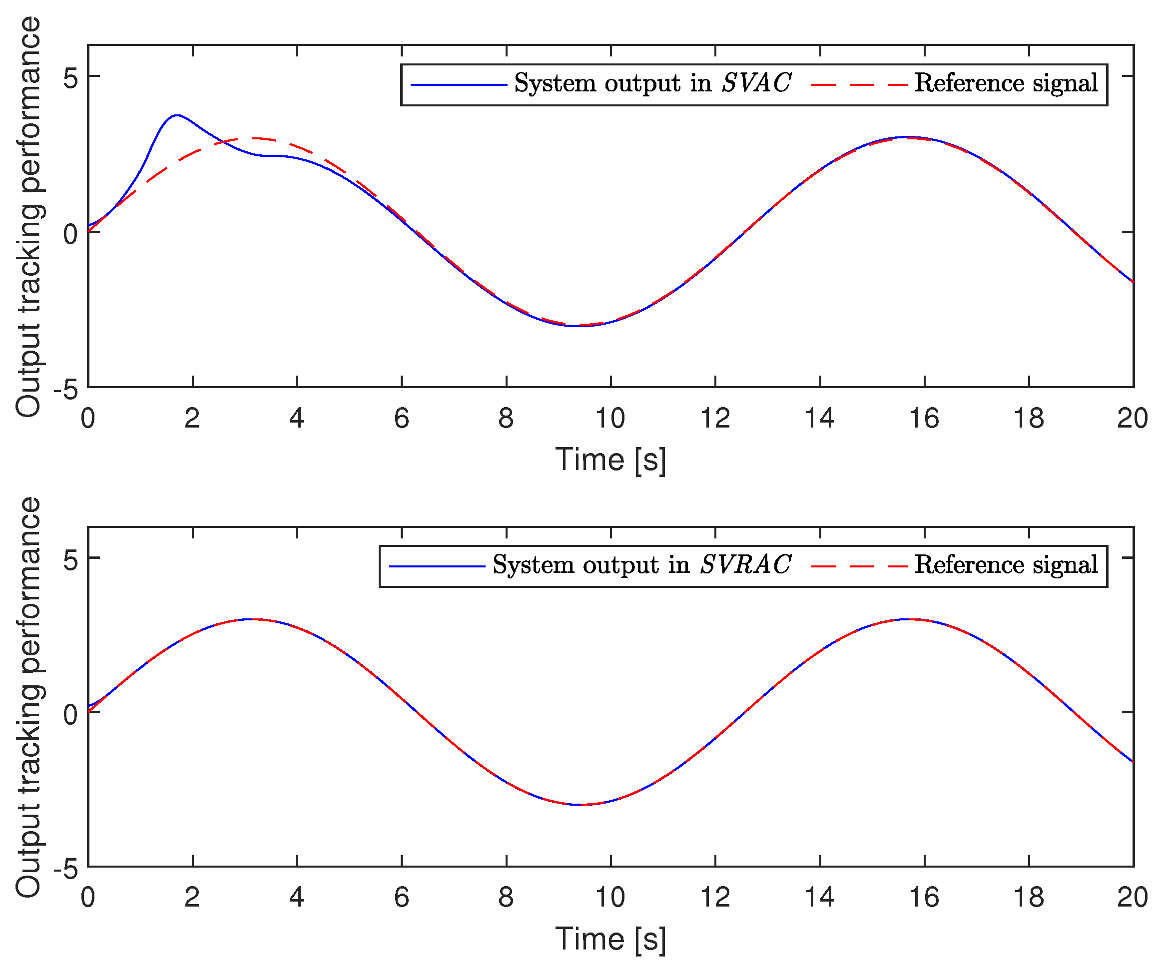
The system’s initial states are set to ${\varpi }_1\left(0\right)=0.2$, ${\varpi }_2\left(0\right)=0.5$, and ${\varpi }_3\left(0\right)=0.6$, with the chosen reference signal being ${\varpi }_r\left(t\right)=3sin\left(0.5t\right)$.

The sliding variable is formulated as follows:

$$\begin{array}{c}\hfill \rho \left(t\right)=3\left({\varpi }_1\left(t\right)-3sin\left(0.5t\right)\right)+5\left({\varpi }_2\left(t\right)-1.5cos\left(0.5t\right)\right)+{\varpi }_3\left(t\right)+0.75sin\left(0.5t\right).\end{array}$$

(26)

The comparative SVAC is defined as

$$\begin{array}{c}\hfill u=-13\rho \left(t\right)-{\widehat{V}}_L^T\left(t\right)O\left(\overline{\varpi }\right),\end{array}$$

(27)

and the proposed SVRAC is expressed as

$$\begin{array}{c}\hfill u=-13\rho \left(t\right)-{\widehat{V}}_L^T\left(t\right)O\left(\overline{\varpi }\right)-5\mathrm{sgn}\left(\rho \right).\end{array}$$

(28)

The NN for approximating $\widehat{L}\left(\overline{\varpi }\right)={\widehat{V}}_L^T\left(t\right)O\left(\overline{\varpi }\right)$ is configured with 24 neurons, with the centers evenly distributed across the range $[-8,8]$. The basis function is defined as follows:

$$\begin{array}{c}\hfill O_i\left(\overline{\varpi }\right)=\exp \left[{\displaystyle \frac{\parallel {[{\varpi }_1,{\varpi }_2,{\varpi }_3]}^T-{[8,8,8]}^T+\frac{2}{3}{[i,i,i]}^T{\parallel }^2}{3}}\right],i=1,\cdots ,24.\end{array}$$

(29)

The weight adaptive law corresponding to (12) is given by

$$\begin{array}{c}\hfill {\dot{\widehat{V}}}_L\left(t\right)=-\left(O\left(\overline{\varpi }\right)O^T\left(\overline{\varpi }\right){\widehat{V}}_L\left(t\right)+8{\widehat{V}}_L\left(t\right)\right),\end{array}$$

(30)

with the initial weight value specified as ${\widehat{V}}_L\left(0\right)={\left[0.6\right]}_{24\times 1}$.

The simulation results are presented in Figure 1, Figure 2, Figure 3, Figure 4 and Figure 5. Figure 1 illustrates that, compared to the SVAC scheme, our proposed SVRAC exhibits significantly improved tracking performance, particularly during the initial phase of the simulation. Figure 2 demonstrates that the tracking error under SVRAC is significantly smaller and converges to a small neighborhood near zero.

Table 1. Performance comparison of control methods.

Control Method	First-Time Settling Time for $\mathit{\beta }\left(\mathit{t}\right)<0.01$	Average Error
SVAC	0.36 s	0.0270
SVRAC	0.35 s	0.0021

shows that SVRAC achieves a faster convergence speed and a smaller tracking error compared to SVAC, highlighting its superior performance in ensuring precise and efficient system control. Figure 3 shows the norm of NN weight over time for the SVRAC scheme. The weight norm rapidly decreases and stabilizes close to zero, indicating fast convergence of the NN training process. Figure 4 shows that, despite some noticeable fluctuations, the control input under the SVRAC scheme stays bounded throughout the simulation. 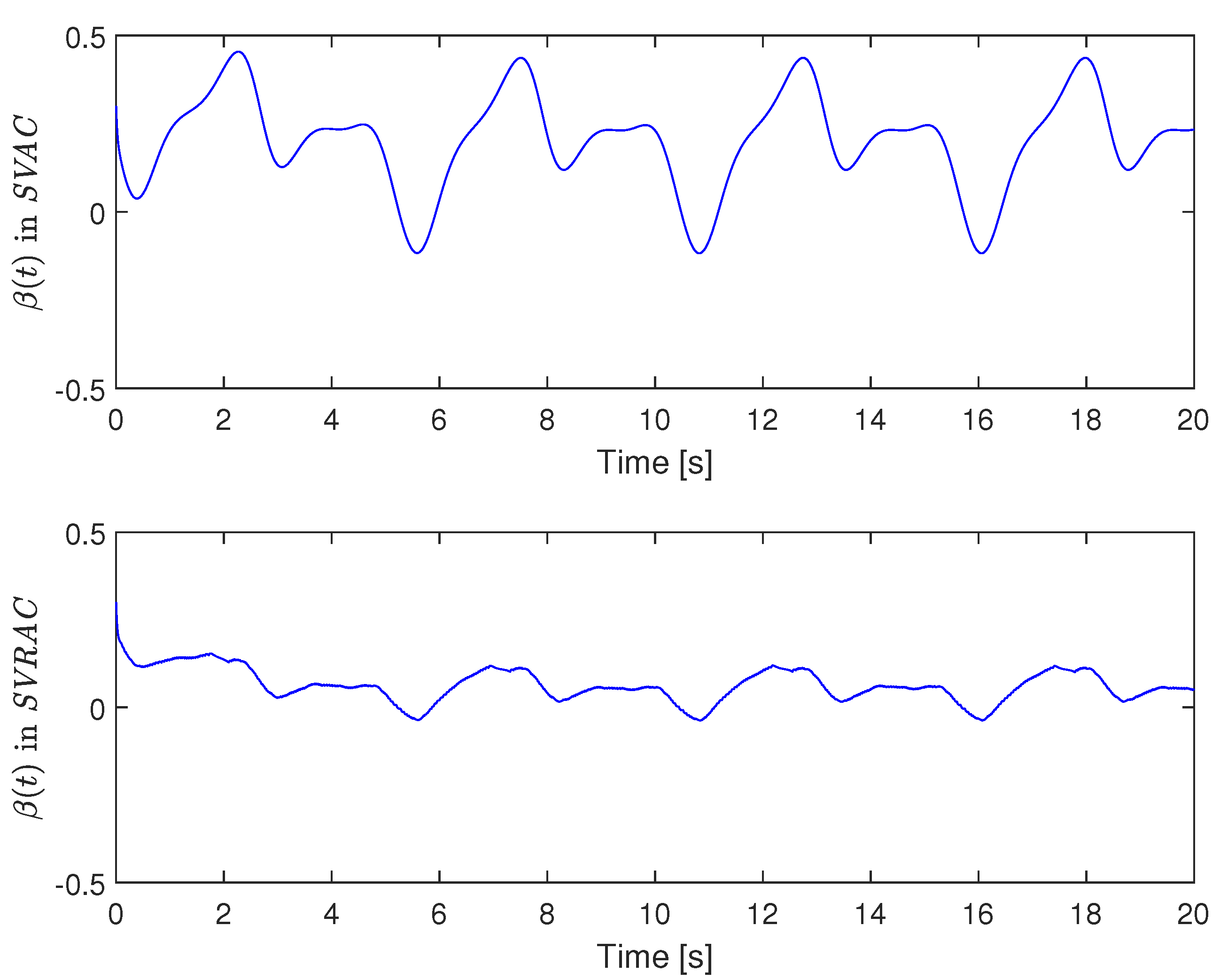Figure 5 presents the trajectory of the sliding variable in the SVRAC scheme. In summary, Figure 1, Figure 2, Figure 3, Figure 4 and Figure 5 further validate the effectiveness of the proposed SVRAC in numerical simulations. The results consistently demonstrate improved tracking performance, reduced tracking error, bounded NN weight, and stable control input, confirming the robustness and adaptability of the proposed control approach.

4.2. Example 2 (Application Example)

Consider the single-link rigid manipulator, which is governed by the following second-order nonlinear differential equation:

$$\begin{array}{c}\hfill M{L}^2\ddot{\eta }+b\dot{\eta }+ML{g}_{0}cos\left(\eta \right)=u,\end{array}$$

(31)

where the system parameters are detailed in

Table 2. Definition of system parameters.

Parameter	Description
$\eta$	The angle of the link relative to the horizontal direction
$\dot{\eta }$	The angular velocity of the link
$\ddot{\eta }$	The angular acceleration of the link motion
M	The mass of a single link manipulator
L	The length of the link
b	The damping coefficient
$g_0$	Gravitational acceleration

.

Let ${\varpi }_1\left(t\right)=\eta$ and ${\varpi }_2\left(t\right)=\dot{\eta }$. The dynamic Equation (31) can be rewritten in state-space form as follows:

$$\begin{array}{cc}\hfill \dot{{\varpi }_1}\left(t\right)& ={\varpi }_2\left(t\right),\hfill \\ \hfill \dot{{\varpi }_2}\left(t\right)& =-{\displaystyle \frac{g_0}{L}}cos\left({\varpi }_1\right)-{\displaystyle \frac{b}{M{L}^2}}{\varpi }_2\left(t\right)+{\displaystyle \frac{1}{M{L}^2}}u.\hfill \end{array}$$

(32)

The initial conditions are specified as ${\varpi }_1\left(0\right)=0.3$ and ${\varpi }_2\left(0\right)=0.6$. The selected system parameters are $M=5\mathrm{kg}$, $L=0.5\mathrm{m}$, $b=1\mathrm{N}·\mathrm{m}·\mathrm{s}/\mathrm{rad}$, and $g_0=9.81{\mathrm{m}/\mathrm{s}}^2$. Additionally, the reference trajectory for the manipulator is defined by ${\varpi }_r\left(t\right)=4sin\left(1.2t\right)$.

The sliding variable is formulated as

$$\begin{array}{c}\hfill \rho \left(t\right)={\varpi }_1\left(t\right)-4sin\left(1.2t\right)+{\varpi }_2\left(t\right)-4.8cos\left(1.2t\right).\end{array}$$

(33)

The comparative SVAC is defined as

$$\begin{array}{c}\hfill u=-50\rho \left(t\right)-{\widehat{V}}_L^T\left(t\right)O\left(\overline{\varpi }\right),\end{array}$$

(34)

and the proposed SVRAC is expressed as

$$\begin{array}{c}\hfill u=-50\rho \left(t\right)-{\widehat{V}}_L^T\left(t\right)O\left(\overline{\varpi }\right)-30\mathrm{sgn}\left(\rho \right).\end{array}$$

(35)

The NN for approximating $\widehat{L}\left(\overline{\varpi }\right)={\widehat{V}}_L^T\left(t\right)O\left(\overline{\varpi }\right)$ is configured with 36 neurons, with the centers evenly distributed across the range $[-9,9]$. The basis function is defined as follows:

$$\begin{array}{c}\hfill O_i\left(\overline{\varpi }\right)=\exp \left[{\displaystyle \frac{\parallel {[{\varpi }_1,{\varpi }_2]}^T-{[9,9]}^T+\frac{1}{2}{[i,i]}^T{\parallel }^2}{5}}\right],i=1,\cdots ,36.\end{array}$$

(36)

The weight adaptive law corresponding to (12) is given by

$$\begin{array}{c}\hfill {\dot{\widehat{V}}}_L\left(t\right)=-0.8\left(O\left(\overline{\varpi }\right)O^T\left(\overline{\varpi }\right){\widehat{V}}_L\left(t\right)+5{\widehat{V}}_L\left(t\right)\right),\end{array}$$

(37)

with the initial weight value specified as ${\widehat{V}}_L\left(0\right)={\left[0.9\right]}_{36\times 1}$.

Figure 6, Figure 7, Figure 8, Figure 9 and Figure 10 display the simulation results. Figure 6 illustrates the tracking performances under SVAC and SVRAC, respectively. Additionally, Figure 7 shows the corresponding tracking errors. The results presented in

Table 3. Performance comparison of control methods.

Control Method	First-Time Settling Time for $\mathit{\beta }\left(\mathit{t}\right)<0.01$	Average Error
SVAC	5.24 s	0.2001
SVRAC	5.15 s	0.0632

quantitatively validate the effectiveness of the proposed SVRAC method. It is evident that, compared to SVAC, the proposed SVRAC demonstrates superior tracking performance, with a shorter convergence time and a significantly smaller tracking error. Figure 8 presents the evolution of the NN weight norm over time for the SVRAC scheme. The weight norm initially decreases sharply and then remains close to zero, suggesting that the NN parameters quickly converge and stabilize. The bounded nature of SVRAC is depicted in Figure 9. Furthermore, Figure 10 plots the trajectory of the sliding variable within the SVRAC scheme. Overall, Figure 6, Figure 7, Figure 8, Figure 9 and Figure 10 collectively validate the effectiveness of the proposed SVRAC in engineering simulation. These results consistently demonstrate that SVRAC not only enhances tracking performance but also reduces tracking error and improves overall system stability. This empirical evidence reinforces the robustness and adaptability of the proposed strategy, confirming its efficacy in effectively managing uncertainties.

5. Conclusions

This article presents a robust control framework, Sliding Variable-Based Robust Adaptive Control (SVRAC), for canonical nonlinear system with unknown dynamic and control gain functions. By integrating NN approximations with SMC principles, the proposed SVRAC overcomes the limitations of traditional SMC and adaptive control methods. Unlike conventional approaches, SVRAC simplifies the controller design by eliminating the need for equivalent and switching controls while enhancing robustness and adaptability through a robustness adjustment term. Theoretical validation through Lyapunov stability analysis confirms that the system achieves Semi-Globally Uniformly Ultimately Bounded (SGUUB) error behavior, with the tracking error converging to a small neighborhood around zero. Numerical and engineering simulations further demonstrate the practical effectiveness of SVRAC in achieving superior tracking performance, faster convergence, and enhanced robustness compared to traditional methods. Despite its strengths, the use of a discontinuous sign function in the robustness adjustment term may lead to chattering, which can affect the smoothness of the control input. Future work will focus on mitigating this effect by developing chattering-free control techniques and extending the proposed framework to address more complex discrete-time and stochastic systems. These enhancements will further broaden the applicability of SVRAC in advanced engineering systems. Overall, the proposed SVRAC framework provides an efficient and practical solution for managing uncertainties in nonlinear systems, offering significant potential for applications in robotics, aerospace, and other dynamic control environments.

References

- Fu, J.; Liu, X.; Liu, Y.; Chen, Z.; Yao, B. Fast and accurate tracking control of robotic manipulators subject to state constraints and input saturation by effectively integrating planning strategies. ISA Trans. 2024, 149, 373–380. [Google Scholar] [CrossRef]
- Fei, J.; Wang, H.; Fang, Y. Novel neural network fractional-order sliding-mode control with application to active power filter. IEEE Trans. Syst. Man Cybern. Syst. 2021, 52, 3508–3518. [Google Scholar] [CrossRef]
- Herrera, M.; Camacho, O.; Leiva, H.; Smith, C. An approach of dynamic sliding mode control for chemical processes. J. Process Control 2020, 85, 112–120. [Google Scholar] [CrossRef]
- Xu, Q.; Zhao, H. Sliding Mode Control of Uncertain Switched Systems via Length-Limited Coding Dynamic Quantization. Mathematics 2024, 12, 3749. [Google Scholar] [CrossRef]
- Li, J.; Zhao, Z.; Qin, X. Adaptive sliding mode control using a novel fully feedback recurrent neural network for quad-rotor UAVs. Neurocomputing 2024, 610, 128592. [Google Scholar] [CrossRef]
- Liu, C.; Wei, T.; He, X.; Li, X. Sliding-mode control for target tracking of omnidirectional mobile robots subject to impulsive deception attacks. Chaos Solitons Fractals 2024, 187, 115439. [Google Scholar] [CrossRef]
- Hu, J.; Zhang, H.; Liu, H.; Yu, X. A survey on sliding mode control for networked control systems. Int. J. Syst. Sci. 2021, 52, 1129–1147. [Google Scholar] [CrossRef]
- Roy, S.; Baldi, S.; Fridman, L.M. On adaptive sliding mode control without a priori bounded uncertainty. Automatica 2020, 111, 108650. [Google Scholar] [CrossRef]
- Qiu, Q.; Su, H. Distributed adaptive robust containment control for reaction–diffusion neural networks with external disturbances under directed graphs. Neural Netw. 2024, 176, 106363. [Google Scholar] [CrossRef]
- Wang, J.; Zhang, C.; Zheng, C.; Kong, X.; Bao, J. Adaptive neural network fault-tolerant control of hypersonic vehicle with immeasurable state and multiple actuator faults. Aerosp. Sci. Technol. 2024, 152, 109378. [Google Scholar] [CrossRef]
- Chakraborty, A.; Maity, T. An adaptive fuzzy logic control technique for LVRT enhancement of a grid-integrated DFIG-based wind energy conversion system. ISA Trans. 2023, 138, 720–734. [Google Scholar] [CrossRef] [PubMed]
- Zamani Sabzi, H.; Humberson, D.; Abudu, S.; King, J.P. Optimization of adaptive fuzzy logic controller using novel combined evolutionary algorithms, and its application in Diez Lagos flood controlling system, Southern New Mexico. Expert Syst. Appl. 2016, 43, 154–164. [Google Scholar] [CrossRef]
- Liu, H.; Pan, Y.; Cao, J.; Wang, H.; Zhou, Y. Adaptive neural network backstepping control of fractional-order nonlinear systems with actuator faults. IEEE Trans. Neural Netw. Learn. Syst. 2020, 31, 5166–5177. [Google Scholar] [CrossRef]
- Liang, H.; Liu, G.; Zhang, H.; Huang, T. Neural-network-based event-triggered adaptive control of nonaffine nonlinear multiagent systems with dynamic uncertainties. IEEE Trans. Neural Netw. Learn. Syst. 2020, 32, 2239–2250. [Google Scholar] [CrossRef]
- Wen, G.; Dou, H.; Li, B. Adaptive fuzzy leader-follower consensus control using sliding mode mechanism for a class of high-order unknown nonlinear dynamic multi-agent systems. Int. J. Robust Nonlinear Control 2023, 33, 545–558. [Google Scholar] [CrossRef]
- Zhao, H.; Zong, G.; Zhao, X.; Wang, H.; Xu, N.; Zhao, N. Hierarchical sliding-mode surface-based adaptive critic tracking control for nonlinear multiplayer zero-sum games via generalized fuzzy hyperbolic models. IEEE Trans. Fuzzy Syst. 2023, 31, 4010–4023. [Google Scholar] [CrossRef]
- Li, Y.; Tong, S. Adaptive backstepping control for uncertain nonlinear strict-feedback systems with full state triggering. Automatica 2024, 163, 111574. [Google Scholar] [CrossRef]
- Wu, H. Adaptive robust output tracking of uncertain strict-feedback nonlinear systems with full state constraints via control schemes with simple structure. Int. J. Control 2024, 97, 2389–2398. [Google Scholar] [CrossRef]
- Wang, B.; Tian, X.; Xu, R.; Song, C. Threshold dynamics and optimal control of a dengue epidemic model with time delay and saturated incidence. J. Appl. Math. Comput. 2023, 69, 871–893. [Google Scholar] [CrossRef]
- Johansyah, M.D.; Sambas, A.; Hannachi, F.; Hamidzadeh, S.M.; Rusyn, V.; Hidayanti, M.; Foster, B.; Rusyaman, E. Dynamics and Stabilization of Chaotic Monetary System Using Radial Basis Function Neural Network Control. Mathematics 2024, 12, 3977. [Google Scholar] [CrossRef]
- Ding, H.; Wang, Y.; Shen, H. A reinforcement learning integral sliding mode control scheme against lumped disturbances in hot strip rolling. Appl. Math. Comput. 2024, 465, 128407. [Google Scholar] [CrossRef]
- Wang, S.; Cao, Y.; Huang, T.; Chen, Y.; Li, P.; Wen, S. Sliding mode control of neural networks via continuous or periodic sampling event-triggering algorithm. Neural Netw. 2020, 121, 140–147. [Google Scholar] [CrossRef] [PubMed]
- Zhu, J.; Wen, G.; Veluvolu, K.C. Optimized backstepping consensus control using adaptive observer-critic–actor reinforcement learning for strict-feedback multi-agent systems. J. Frankl. Inst. 2024, 361, 106693. [Google Scholar] [CrossRef]
- Han, C.; Qin, K.; Lin, B.; Shi, M.; Li, Z.; Liu, Q. Neural network-based distributed consensus tracking control for uncertain Euler–Lagrange systems over directed topologies. Neurocomputing 2024, 608, 128383. [Google Scholar] [CrossRef]
- Zhu, B.; Liang, H.; Niu, B.; Wang, H.; Zhao, N.; Zhao, X. Observer-based reinforcement learning for optimal fault-tolerant consensus control of nonlinear multi-agent systems via a dynamic event-triggered mechanism. Inf. Sci. 2025, 689, 121350. [Google Scholar] [CrossRef]
- Tong, S.; Li, Y.; Li, Y.; Liu, Y. Observer-based adaptive fuzzy backstepping control for a class of stochastic nonlinear strict-feedback systems. IEEE Trans. Syst. Man Cybern. Part B (Cybern.) 2011, 41, 1693–1704. [Google Scholar] [CrossRef]
- Li, Y.; Tong, S. Event-Triggered Output-Feedback Adaptive Control of Interconnected Nonlinear Systems: A Cyclic-Small-Gain Approach. IEEE Trans. Cybern. 2024, 54, 3239–3250. [Google Scholar] [CrossRef]