Abstract
Spatial discrete data modeling plays a crucial role in geoscientific data analysis, with accuracy and efficiency being significant factors to consider in the modeling of massive discrete datasets. In this paper, an efficient and regularized modeling method, TIN-MQ, which integrates a triangulated irregular network (TIN) and a multiquadric (MQ) function, is proposed. Initially, a constrained residual MQ function and a damped least squares linear equation are constructed, and the conjugate gradient method is employed to solve this equation to enhance the modeling precision and stability. Subsequently, the divide-and-conquer algorithm is used to build the TIN, and, based on this TIN, the concave hull boundary of the discrete point set is constructed. The connectivity relationships between adjacent triangles in the TIN are then utilized to build modeling subdomains within the concave hull boundary. By integrating the OpenMP multithreading programming technology, the modeling tasks for all subdomains are dynamically distributed to all threads, allowing each thread to independently execute the assigned tasks, thereby rapidly enhancing the modeling efficiency. Finally, the TIN-MQ method is applied to model synthetic Gaussian model data, the submarine terrain of the Norwegian fjords, and elevation data from Hunan Province, demonstrating the method’s good fidelity, stability, and high efficiency.
Keywords:
triangulated irregular network; multiquadric function; massive scattered data; stable modeling MSC:
86-10
1. Introduction
Geoscientific data collection is influenced by various objective factors, often resulting in the collection of data points that are discrete and irregularly distributed. To facilitate the modeling and analysis of these data, spatial interpolation methods are commonly employed to densify discrete data and create regularly distributed spatial datasets [1,2,3]. There are several types of spatial interpolation methods, such as kriging, minimum curvature, radial basis functions, natural neighbors, and inverse distance weighting. Each method has its advantages and disadvantages in terms of interpolation accuracy, visual representation, parameter sensitivity, and time and memory consumption [4,5,6]. Among them, the kriging method is known for its high modeling precision and strong applicability, and it is widely used in the field of geosciences [7,8,9,10]. However, when dealing with the modeling of massive discrete datasets, the accuracy and efficiency of the kriging method are significantly affected by the neighborhood search algorithms used to construct sample subsets [11,12]. For mature geoscientific analysis software such as ArcGIS and Surfer16, neighborhood search algorithms predominantly use fixed number and fixed radius methods [13]. These algorithms are time-consuming in their search processes, and, despite the use of multithreading technology, the modeling processes of kriging and radial basis function methods still require significant computational time.
The multiquadric (MQ) function was first proposed by Hardy in 1968; since then; more and more efforts have been made to develop radial basis methods, and breakthroughs have been achieved in the types of basis function [14,15,16,17], adaptive selection shape parameters [18,19,20], and selection of the interpolation points [21] and so on, and it is widely believed that the radial basis function method is an effective way to solve multivariate scattered data approximation problems [22]. In the family of radial basis functions, the MQ function is widely utilized due to its excellent conformality, smoothness, continuity, and its ability to approximate the local features of discrete datasets effectively. This function has found extensive application in fields such as computational science [23,24], geology [25], engineering problems [26], and geographic information systems [27]. However, when the MQ function is used to model discrete datasets that are unevenly distributed or have missing boundaries, the resulting system of multivariate quadratic equations becomes severely ill-conditioned, leading to distortions in the local modeling outcomes [28]. To effectively enhance the stability of MQ function modeling, one feasible solution to overcome this challenge is presented by improving the MQ function through the application of first- and second-order roughness constraints, integrating trend surface functions, or adjusting the shape parameters [29,30].
The construction of neighborhood search algorithms for subsets of discrete points also plays a crucial role in affecting the quality and efficiency of modeling, particularly for massive sets of discrete data. In digital terrain modeling, triangulated irregular networks (TINs) are commonly used to represent continuous terrain surfaces and can reflect the original terrain details. These networks possess high surface reconstruction accuracy, and the nearest node set is self-defined geometrically [31,32]. The selection and number of sample points depend solely on their local distribution; even if the distance between some scattered points is relatively large, or their distribution exhibits high anisotropy, it can still be reflected in the topological relationships of local triangles. For this reason, using the connectivity relationships between triangles in the TIN model to construct local sets of discrete points is considered a relatively satisfactory approach for local interpolation schemes.
To enhance the precision and efficiency in modeling massive sets of discrete data, an efficient and stable modeling method, TIN-MQ, which integrates a triangulated irregular network with an MQ function, is proposed in this paper. To improve the stability of the MQ function in modeling, a constrained residual MQ function is first constructed, and the ill-conditioned coefficient equations are solved using the damped least squares conjugate gradient method, ensuring that areas with large gradient changes possess higher modeling accuracy. To enhance the modeling efficiency and depict the model boundary morphology, the convex hull boundary of the discrete point set is constructed based on the TIN model, and the connectivity relationships between adjacent triangles in the TIN model are utilized to search for discrete point sets within the convex hull boundary for the construction of multiple local quadratic surfaces. Subsequently, the subdomain surface stitching and OpenMP multithreading computation techniques are employed to further enhance the modeling efficiency. Finally, modeling experiments conducted on synthetic Gaussian model data, the submarine terrain of the Norwegian fjords, and actual elevation data from Hunan Province, and comparative analyses with the kriging method and radial basis function method in the Surfer software, demonstrate that the proposed method offers good modeling accuracy and high efficiency.
2. Methodology
The principles of the TIN-MQ modeling method are as follows. (1) A new stable MQ function is constructed, and the damped least squares linear equation based on this method is derived, along with the iterative format of its conjugate gradient solution. (2) The TIN model of the discrete dataset is constructed using the divide-and-conquer algorithm, and reasonable boundary points are progressively searched inward based on the convex hull boundary of the TIN model. (3) By integrating the OpenMP multithreading programming technology, an efficient modeling method for massive discrete datasets is implemented within the concave hull boundary, merging the TIN model with the MQ function.
2.1. Modeling Method of MQ Functions with Stability
Based on discrete data points , a multivariate quadratic surface function [13] can be constructed to reflect the local features of the data points as
where is a quadratic surface function, is the quadratic surface coefficient, and is the shape parameter (used to adjust the smoothness of the quadratic surface). To ensure that the constructed mathematical surface approximates the real surface as closely as possible, the shape parameter is typically chosen to be a small value. In this paper, it is selected as , where represents the diameter of the minimum circumscribed circle containing all data points.
To determine the quadratic surface coefficient , the discrete points are substituted into Equation (1), with . Equation (1) can be presented in matrix form as
Solving Equation (2) yields the MQ coefficients , and then the MQ surface will be expressed analytically by Equation (1).
Equation (2) indicates that the elements of matrix are composed of the planar distances between data points. The nature of the equation often relates to the planar distribution characteristics of the data points and the amplitude of changes in the field value . When the data points are extremely unevenly distributed or when there are missing data, as well as when varies significantly, distortions can easily arise in the solution of the quadratic surface coefficients, which in turn leads to distortions in the constructed multivariate quadratic surfaces. Based on this, a constrained residual MQ function is proposed as
where the function is constructed from the discrete points , and is a constant to be determined; it can enhance the stability of the MQ function.
To determine the coefficients and the correction term , Equation (3) is evaluated by substituting the discrete points , setting , and considering the constraint conditions. Equation (3) can be presented in matrix form as
where , , .
To ensure the stability of the solution for Equation (4), an objective function with imposed constraints is constructed based on the damped least squares method. The objective function of MQ can be expressed as
where is the Euclidean norm; is a damping factor and it is set to be equal to . It controls the trade-off between surface smoothness and fidelity to the result. To minimize the function , letting the first derivative of with respect to be equal to zero, we obtain
Then, we can obtain the linear equation
The damped least squares conjugate gradient method has a strong solving ability and is widely used in inverse problems [32]; consequently, we choose it to solve Equation (7). First, we initialize the initial solution , and denotes the residual of the basis equation, so the initial residual is . is the gradient vector, is the conjugate direction vector, and their initial values are . The pseudocode description of this iterative process is shown in Algorithm 1, where the maximum iteration count ; and , respectively, are the modified factors of the solution vector and the conjugate direction vector .
After obtaining the quadratic surface coefficients for the residual surface, according to Equation (3), the resulting multiquadratic surface function defined by the discrete data points can be expressed as
| Algorithm 1. Pseudocode for the iterative solution of linear equations using the damped least squares conjugate gradient method |
| INPUT: (coefficient matrix), (vector), (damping factor), (stopping criterion) OUTPUT: (solution vector) 1. FOR DO 2. 3. 4. 5. 6. 7. IF BREAK 8. 9. END FOR |
2.2. Constructing the Concave Hull Boundary of Discrete Points According to the TIN Model
The outer boundaries of massive sets of discrete points are typically irregular. To enhance the modeling efficiency and reduce model redundancy, it is usually necessary only to compute the field values of model grid nodes within the boundary. Therefore, constructing the concave hull boundary of discrete point sets is essential. The main methods for the construction of concave hulls include the ball pivoting and edge pivoting techniques. Since the TIN model forms the basis for the efficient modeling of massive discrete datasets in this paper, the concave hull boundary of discrete point sets is constructed using the TIN model. The principles of the algorithm are as follows.
- Based on the planar coordinates of discrete points, the maximum convex hull containing the Delaunay triangulation network (i.e., the TIN model, as shown in Figure 1a) [33] is constructed using the divide-and-conquer algorithm. During the construction of the TIN model, the topological relationships of the triangulation network are recorded, including the indices of triangles, the indices of triangle vertex coordinates, and the triangles adjacent to each vertex. Additionally, the average distance between adjacent discrete points in the triangulation network is calculated.
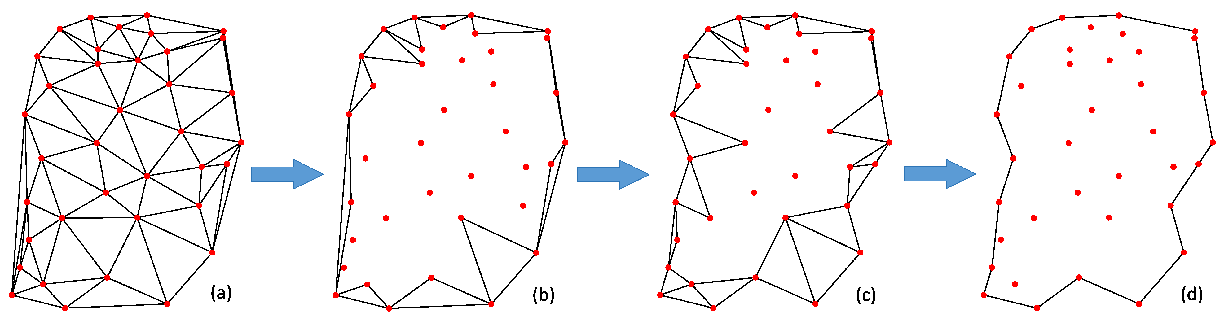
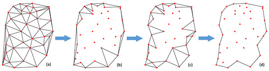 Figure 1. Schematic of the concave hull construction process: (a) TIN model, (b) triangle queue T with convex hull boundary, (c) triangle queue T with concave hull boundary, (d) concave hull boundary.
 - Triangles that belong to the convex hull boundary (as illustrated in Figure 1b) are identified and added to the boundary triangle queue T.
- A triangle is retrieved from T, and the following conditions must be met: ① if one edge AB is on the boundary, and the length of AB exceeds (the pre-set maximum length), then the two triangles adjacent to the internal edges BC and CA of are added to T, and is removed from T; ② if two edges AB and BC are on the boundary, and the length of AB or BC exceeds and the number of triangles connected to vertex B is greater than 1 (indicating that point B is not an isolated point), then the triangle adjacent to the internal edge CA is added to the T, and is removed from T. This process is repeated, extracting triangles from T and checking if they meet conditions ① and ② until no triangles in T satisfy either condition, ultimately resulting in a triangle queue T that forms a concave hull boundary (as shown in Figure 1c).
- Boundary edges are extracted from the T that forms the concave hull, and these edges are sequentially connected in either a counterclockwise or clockwise direction to construct an ordered list for the concave hull boundary (as shown in Figure 1d).
The algorithm is capable of constructing boundary lists for discrete point sets that include multiple local domains with high efficiency. The shape of the boundary is dependent on its maximum limiting length, . If is large, the boundary generated is the maximum convex hull. If is less than , it may be challenging to generate an effective boundary. Therefore, should be greater than and should be reasonably set according to practical needs.
2.3. Efficient Modeling Approach of MQ Function Combined with TIN Model
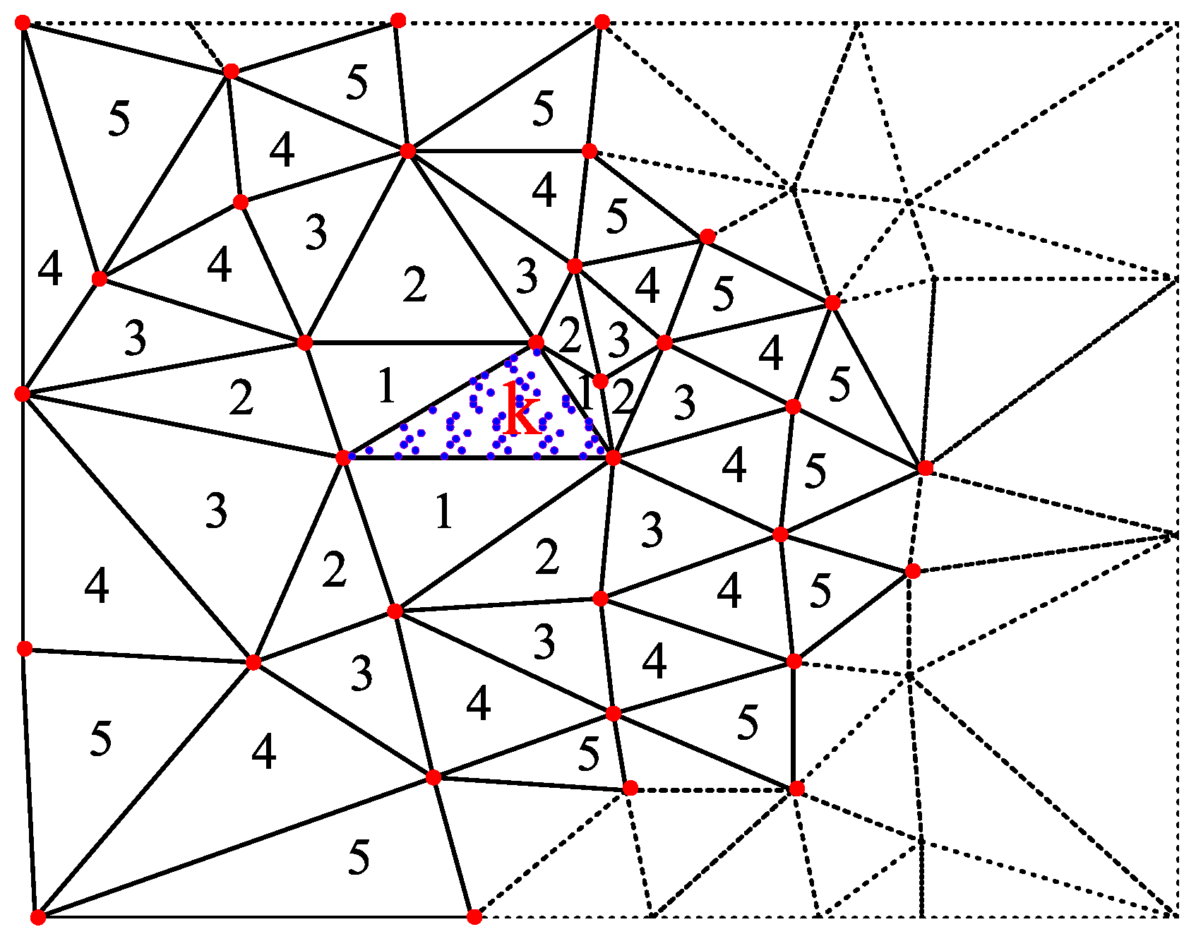
When the volume of the modeling data in a research area is extremely large, modeling failure is often caused by attempting to construct an MQ surface using all data points due to the enormous scale of Equation (4). This significantly limits the capability of the global MQ method to model large datasets. Consequently, based on the TIN model, the entire research area D is divided into M overlapping subdomains , which are the support domains for the calculation of the MQ function, as shown in Figure 2, where M refers to the number of triangles within the concave hull of the TIN model described in Section 2.2, purple dots are the nodes to be interpolated, and numbers represent outward search depths. Each subdomain is defined by an area covered by several triangles expanding outward from any given triangle k. Known discrete points on subdomain are then selected, and a local MQ surface is constructed using the stable MQ function outlined in Section 2.1. Finally, the local MQ surfaces from each subdomain are superimposed to form a global MQ surface. To calculate the function value of an interpolation point within k triangle, we substitute its coordinates into the corresponding MQ function ; the other MQ function values are zero for this point.
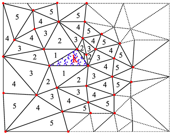
Figure 2.
Constructing subdomain by expanding outward from triangle k.
The key to enhancing the efficiency of MQ modeling using Equation (9) lies in fully utilizing the efficiency in constructing subdomains with the TIN model. Based on the stable MQ function in Equation (8), and incorporating the topological relationships of the triangles recorded during the construction of the TIN model as described in Section 2.2, a comprehensive process is presented for the construction of a global surface by superimposing subdomain MQ surfaces.
- Initially, the connectivity relationships between triangles in the TIN model are stored in the array TriNet, and the topological depth of the subdomain triangulation network, TopoDepth, is set. In practice, this can be chosen based on the uniformity of the distribution of discrete points (e.g., between 3 and 9). When a value of 5 is selected, the area covered by the subdomain is as shown in Figure 2.
- In the TIN model, a triangle k is selected and used as the center to gradually expand outward (as shown in Figure 2). The triangles obtained are sequentially placed into the container LocalTriangles until the topological depth, TopoDepth, is satisfied, at which point the subdomain is determined. The pseudocode for the recursive function of the topological process is presented in Algorithm 2, where is the index of the vertices of the triangular element.
- All vertices of the triangles within the subdomain ( vertices) are extracted and placed into the container LocalVertex. Based on Equation (8), a local MQ surface function is constructed asand interpolation is performed on the model nodes within the central triangle k.
- The processes (2) and (3) are repeated until the local modeling of all subdomains is completed. By stitching together the interpolation results of the central triangles of all subdomains, the modeling of the entire research area is ultimately completed, and the modeling results are stored in the container ModelData.
| Algorithm 2. Pseudocode for the topological process recursion function |
| INPUT: TopoDepth, k, TriNet OUTPUT: LocalTriangles function GetLocalTriangles (TopoDepth, k, TriNet, LocalTriangles) 1. IF TopoDepth==0 RETURN 2. FOR DO 3. 4. IF LocalTriangles.push_back(ik) 5. ELSE CONTINUE 6. GetLocalTriangles (, , TriNet, LocalTriangles) 7. END FOR END FUNCTION |
3. Parallel Implementation of Modeling Method
Based on the stable MQ function modeling method integrated with the TIN model described above, regularized and efficient modeling software for massive discrete datasets has been designed and developed using the VC++ development platform and Open Multi-Processing (OpenMP) shared memory programming technology. The implementation steps of parallel modeling are as follows.
Step 1: Data Import and Parameter Setting.
- Load discrete data records . Display the approximate distribution of discrete points in the program window and show the range of distribution for and the minimum and maximum limits for the modeling result z.
- Construct the TIN model. Record the topological information of the triangular network and calculate the average distance between adjacent discrete points in parallel.
- Build the convex hull boundary of the TIN model. Adjust the maximum boundary limit length with reference to the average distance of adjacent discrete points, perform multiple calculations, check whether the convex hull boundary is reasonable, and output the boundary data file (*.bln).
- Set the topological depth, TopoDepth, of the subdomain triangular network. Select from the range of 3 to 9, with a default choice of 5.
- Set the number of modeling nodes and in the x and y directions. To ensure high-quality modeling, try to make the scale of the modeling unit smaller than the average distance between adjacent discrete points.
Step 2: Parallelization of Modeling Method.
- The modeling nodes contained within each triangle are determined based on the relative position relationship between the modeling nodes and the TIN model (as illustrated in Figure 3). For modeling node P and (as shown in Figure 3), if conditions , , and are met, it is indicated that point P is located on the left side of each edge of the triangle, either within or on the edge of the triangle. Otherwise, tracking continues in the direction of the side where the cross-product is less than 0 (to the right side of this edge). If the tracking reaches the boundary without locating the triangle to which point P belongs, this indicates that the point lies outside the concave hull boundary, and no interpolation is performed for nodes outside this boundary. The modeling nodes contained in the triangle numbered k are placed into the container ModelNodesInTri, and the number of model nodes contained in the k-th triangle is denoted as .
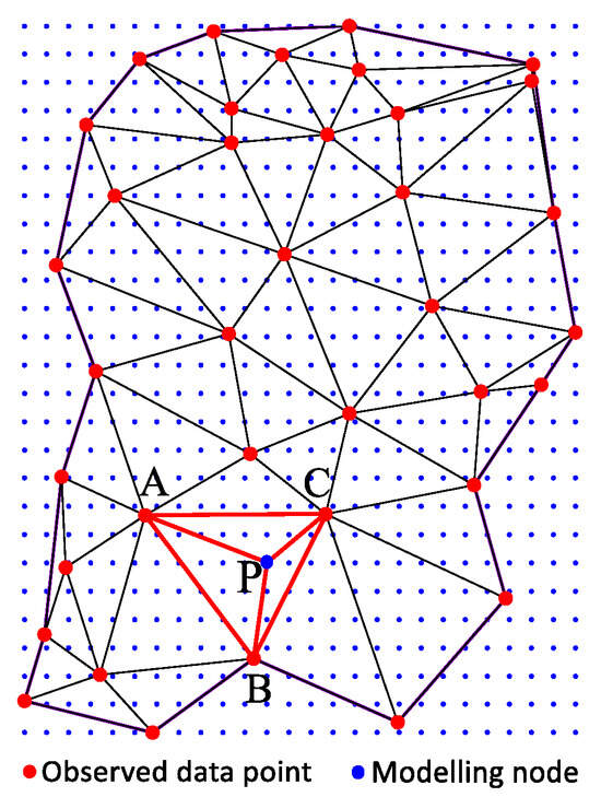 Figure 3. Relative position relationship between modeling nodes and the TIN model.
 - Parallelization of modeling. The modeling tasks of subdomains are independent of each other and can be dynamically allocated to multiple threads to improve the computational efficiency. The pseudocode for parallel computation is shown in Algorithm 3.
Step 3: Model Output. The output data format is *.grd for the modeling results.
| Algorithm 3. Pseudocode for parallel modeling computation |
2. #pragma omp parallel for private (LocalTriangles, LocalVertex, w) schedule (dynamic) 3. FOR DO 4. IF CONTINUE 5. IF () THEN 6. GetLocalTriangles (, i, TriNet, LocalTriangles) 7. ELSE 8. GetLocalTriangles (TopoDepth, i, TriNet, LocalTriangles) 9. END IF
13. 14. FOR DO 15. xx = LocalVertex[i].x-ModelData[ModelNodesInTri[k][j]].x 16. yy= LocalVertex[i].y-ModelData[ModelNodesInTri[k][j]].y 17. 18. END FOR // Constrain the interpolation result . 19. IF THEN 20. ELSE IF THEN 21. END IF 22. ModelData[ModelNodesInTri[k][j]]. 23. END FOR 24. END FOR |
4. Modeling Experiment
The proposed method is applied to both synthetic and field data modeling in this section. In comparison with established conventional approaches, as seen in the commercial software suite Surfer, we aim to evaluate the proposed method’s modeling precision, stability, and performance. All parameters are the default settings of the Surfer software.
4.1. Accuracy Validation on a Synthetic Model
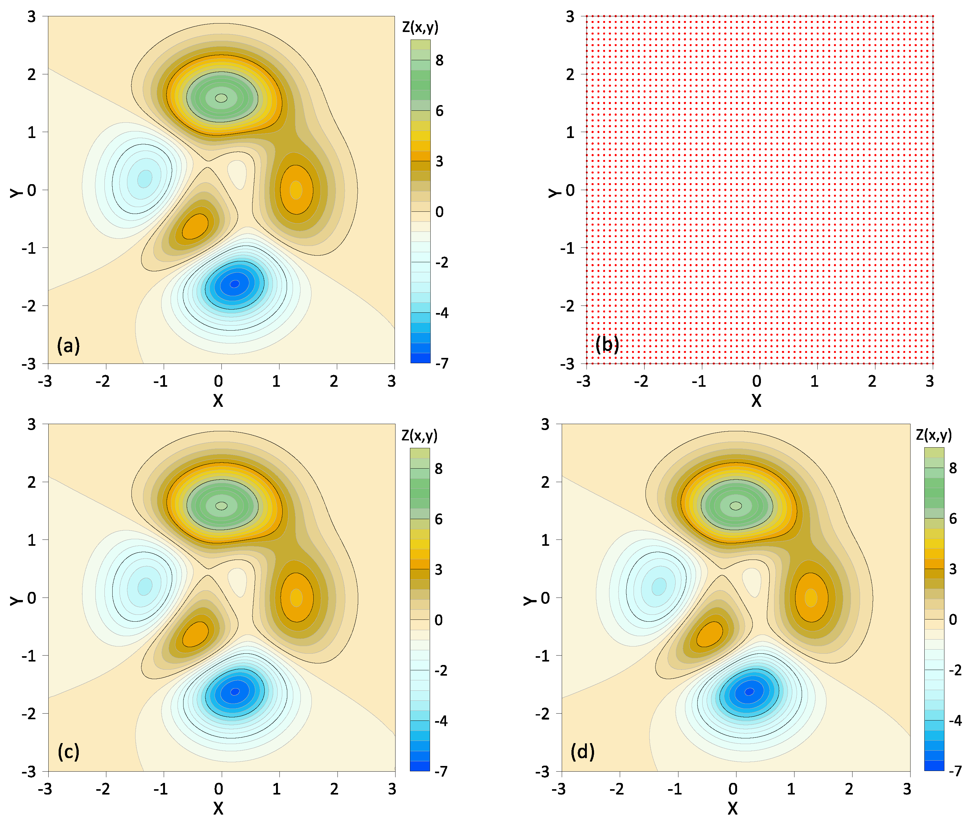
To verify the accuracy of the TIN-MQ method, we choose the Gaussian synthetic model defined by [17]. The analytical geometry is according to Equation (11), and the analytical contour in the domain is presented in Figure 4a.
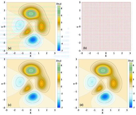

Figure 4.
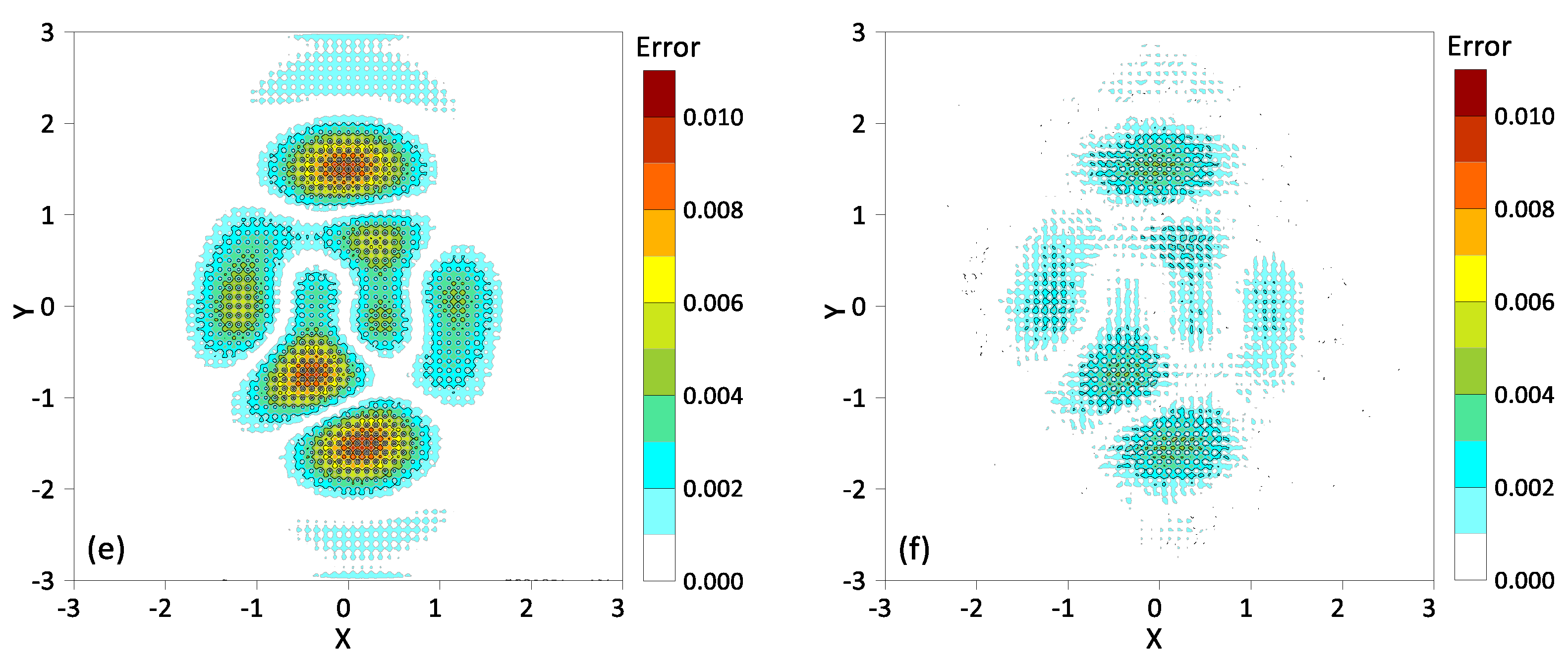
The modeling results from 3271 discrete points by the kriging method and TIN-MQ. (a) Analytical solution, (b) 3271 discrete points, (c) modeling results of kriging method, (d) modeling results of TIN-MQ method, (e,f) absolute errors of the modeling results on the 361,201 modeling points for the kriging and TIN-MQ methods, respectively.
We designed one group of scattered data with 3271 (with 61 points evenly sampled with a 0.1 step length in both the x and y directions) discrete points to reconstruct the contour model defined by 361,201 nodes (with 601 points evenly sampled with a 0.01 step length in both the x and y directions). The details of the discrete points for the modeling test are indicated in Figure 4b.
The accuracy of the TIN-MQ method is validated by the ordinary kriging method. Figure 4c,d show the modeling results on the 361,201 nodes modeling from 3271 discrete points by the kriging method and TIN-MQ method, respectively. It can be observed that the modeling results of the two methods are generally consistent with the analytical results, with no significant differences. However, there are differences in the absolute errors between both methods and the analytical solution, as shown in Figure 4e,f, which show the absolute errors for the kriging and TIN-MQ methods, respectively. Table 1 further lists the average errors and maximum errors for the different methods.

Table 1.
Absolute errors of the kriging and TIN-MQ methods on the synthetic model.
As shown in Figure 4e,f, the absolute errors of these two methods occur at the convex hull of the conical surface. As indicated in Table 1, both the average error and maximum error decrease with the increased number of the original sampling data, which aligns with the fact that the interpolation accuracy is positively related to the density of observed data. The TIN-MQ method has small absolute errors, while the kriging method has the largest average error and maximum error.
This case validates the feasibility of the TIN-MQ method, and it demonstrates superior computational accuracy compared to the kriging method.
4.2. Stability Validation in the Seabed Terrain Modeling of a Fjord in Norway
To verify the stability of the algorithm proposed in this paper, a modeling analysis is conducted using the seabed topography data from a Norwegian fjord as an example, and it is compared with the ordinary kriging method and the MQ radial basis function (RBF) method provided in the Surfer software. The dataset comprises 320,947 data points within the range of , with an average point spacing of 59 m and an elevation range of . It defines 4,004,001 nodes (uniformly discretized into 2000 cell intervals along the x- and y-axes, with cell sizes of 32.1 m and 29.2 m, respectively) and constructs the seabed topography model within the convex hull boundary.
Figure 5a–c show the mapping results of the 4,004,001 data points for the kriging method and MQ-RBF method (using the Surfer software) and the TIN-MQ method, respectively.

Figure 5.
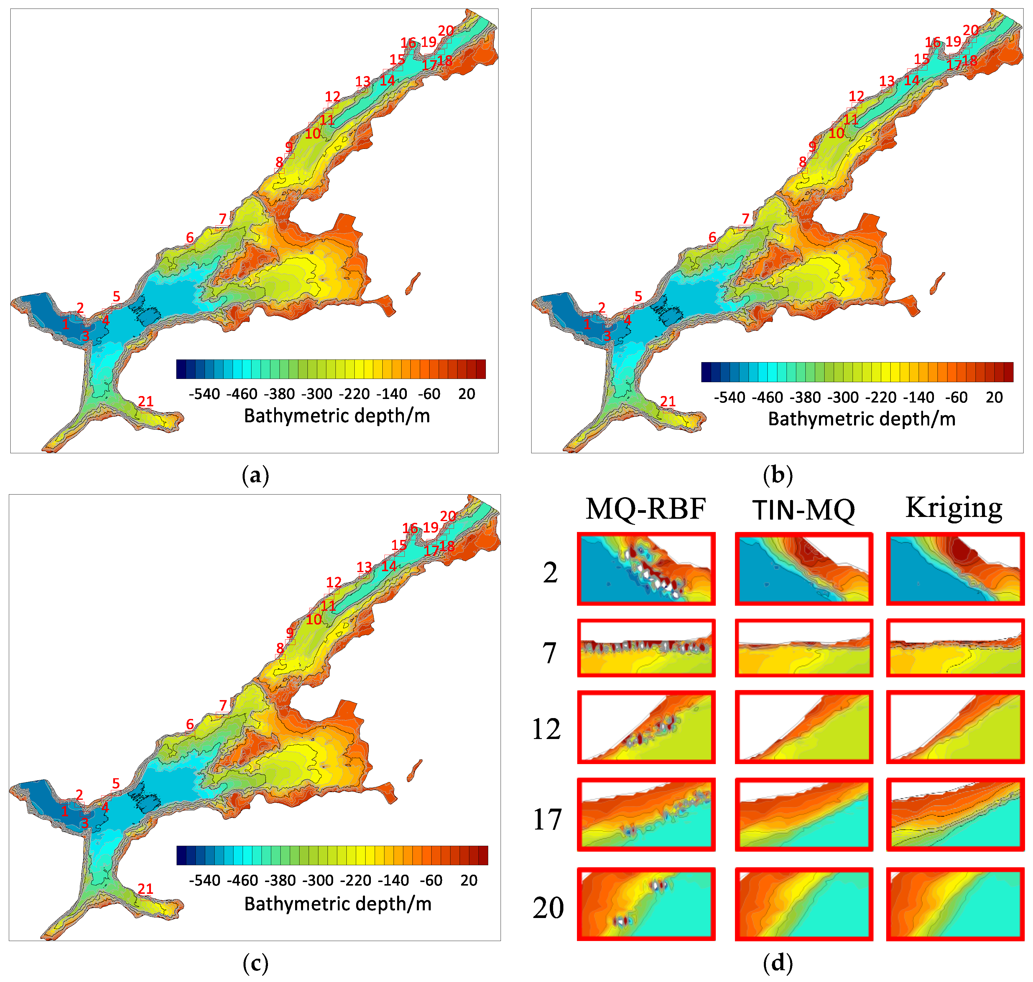
Stability testing of modeling for underwater topography in a Norwegian fjord. (a) Kriging. (b) MQ-RBF. (c) TIN-MQ. (d) Comparison of local region modeling results.
In most regions, the modeling results of these three methods are almost identical and reflect the undulating changes in the seabed terrain well. However, in areas near the fjord boundary, where the seabed undulations change significantly, the MQ-RBF method exhibits varying degrees of distortion (21 distorted regions are marked in Figure 5). Figure 5d shows a comparison of the three methods in regions 2, 7, 12, 17, and 20, where the modeling results from the kriging and TIN-MQ methods are consistent, and the contour lines are smooth. There is no significant difference between these two methods; both constructed seabed terrains reflect the fluctuations in the seabed topography with high quality. In contrast, the MQ-RBF method displays erratic changes in values, failing to accurately represent the changes in the seabed terrain. This case demonstrates the stability of the TIN-MQ method proposed in this paper.
4.3. Efficiency Validation of Terrain Modeling for Massive Digital Elevation Data
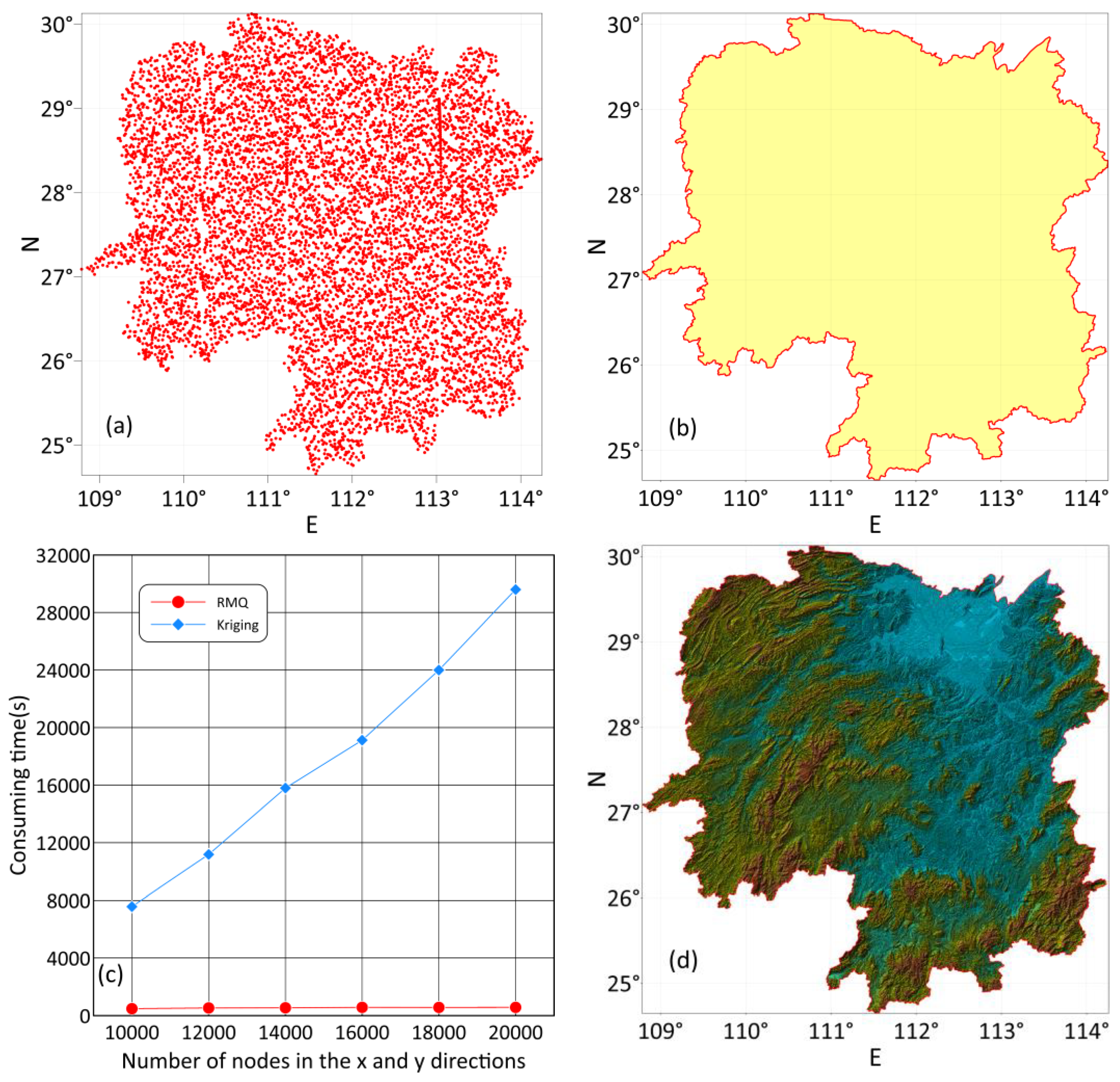
To test the computational efficiency of the TIN-MQ method in modeling massive datasets, we selected digital elevation data from Hunan Province () for this experiment. This dataset contained 27,923,061 discrete points, covering the geographic ranges of and . Figure 6a shows the distribution of thinned discrete points from this dataset. Based on the concave hull boundary algorithm outlined in Section 2.2, we set the maximum allowable distance between two boundary points at ten times the average point distance. The constructed concave hull boundary, as shown in Figure 6b, accurately fits the actual boundary contour of Hunan Province.
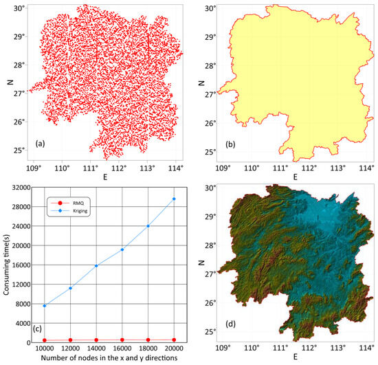
Figure 6.
Efficiency test of elevation modeling for Hunan Province terrain.
To investigate the relationship between the modeling time and the number of modeling nodes, we used various square sizes to discretize the entire planar region into , , , , , and modeling nodes, considerably surpassing the number of discrete points in the dataset. Subsequently, the digital elevation models were constructed using both the TIN-MQ and kriging methods, and the comparative results regarding their time consumption are shown in Figure 6c, revealing that the TIN-MQ and kriging methods required and , respectively. The TIN-MQ method shows only a slight increase in processing time as the node count increases, whereas the kriging method’s time consumption rises linearly with more nodes, clearly demonstrating the higher computational efficiency of the TIN-MQ method. This efficiency confirms that parallel modeling is exceedingly effective. Figure 6d shows the modeling results for nodes using the TIN-MQ method, which finely captures the undulating forms of the terrain.
5. Discussion
This work introduces the TIN-MQ method, an innovative approach that integrates a triangulated irregular network (TIN) with a multiquadric (MQ) function to address the challenges of modeling massive scattered data. The results demonstrate that this method significantly enhances both the accuracy and efficiency of spatial data interpolation compared to conventional techniques such as kriging and radial basis functions (RBFs). This method provides a more comprehensive solution for the handling of large-scale datasets, which is increasingly important in the era of big data in geosciences.
Furthermore, during the research process, we found that the shape parameter(s), the topological depth parameter (TopoDepth), and the solver of the linear equation have a significant impact on the accuracy of the results and the computational efficiency. To further refine the method, the values of these two parameters are also worth investigating in the future. Moreover, the damped least squares conjugate gradient method used in this paper shows better performance in terms of stability compared to other methods in solving ill-conditioned linear equations.
6. Conclusions
In this paper, a new modeling method to improve the modeling quality and efficiency of massive scattered data is proposed, and its accuracy, stability, and high efficiency are validated using synthetic models and practical applications. The main conclusions are as follows.
- An efficient and regularized modeling method integrating the TIN model and MQ functions, referred to as TIN-MQ, is proposed. It is demonstrated in Section 4.1 and Section 4.3 that the modeling error of TIN-MQ is halved compared to the kriging method, and its modeling efficiency exceeds that of kriging by several tens of times. The minimal increase in the computational time with an increase in the number of modeling nodes is identified as the most significant advantage of the TIN-MQ method. This method is noted for its excellent modeling quality and high efficiency, offering broad prospects for application in massive data modeling.
- The stability of MQ function modeling is significantly enhanced by the construction of constrained residual MQ functions and a damped least squares linear equation (Equation (7)), which is solved using the conjugate gradient method, known for its strong anti-ill-conditioning capabilities. Section 4.2 indicates that the stability of the TIN-MQ method surpasses that of the MQ-RBF method in the commercial software Surfer.
- The integration of the TIN model significantly facilitates the determination of concave hull boundaries for discrete points and modeling within these boundaries, effectively shielding against redundant information from outside the boundaries. Additionally, the adjacency of triangles in the TIN model is utilized to construct modeling subdomains, which is key in enhancing the overall modeling efficiency of the TIN-MQ method.
- The dynamic distribution of all subdomain modeling tasks to all threads, enabling the independent execution of assigned tasks by each thread, is achieved using the OpenMP technology. This is a key technology that significantly enhances the modeling efficiency of the TIN-MQ method in this paper.
Author Contributions
Methodology, H.L.; conceptualization, H.L. and J.L.; software, H.L. and Y.Z.; visualization, H.L.; validation, H.L. and Y.Z.; formal analysis, H.L. and X.L.; funding acquisition, H.L.; project administration, H.L. and J.L.; writing—original draft, H.L.; writing—review and editing, H.L., Y.Z., X.L., I.A. and J.L.; investigation, Y.Z. and I.A. All authors have read and agreed to the published version of the manuscript.
Funding
This work was funded by the National Natural Science Foundation of China (Grant No. 42130810 and Grant No. 41774149).
Data Availability Statement
The authors do not have permission to share the data.
Conflicts of Interest
The authors declare that they have no known competing financial interests or personal relationships that could have appeared to influence the work reported in this paper.
References
- Xin, Q.; He, Z. Three dimensional stratum interpolation and visualization based on section and borehole data from jointing the moving least square method and poisson reconstruction method. Earth Sci. Inform. 2020, 13, 1341–1349. [Google Scholar] [CrossRef]
- Zhang, J. Optimization of interpolation parameters based on statistical experiment. Open Geosci. 2022, 14, 880–905. [Google Scholar] [CrossRef]
- Qin, S.; Dai, Z. Interpolation Technique for the Underwater DEM Generated by an Unmanned Surface Vessel. CMES Comput. Model. Eng. Sci. 2023, 136, 3157–3172. [Google Scholar] [CrossRef]
- Yan, L.; Tang, X.; Zhang, Y. High Accuracy Interpolation of DEM Using Generative Adversarial Network. Remote Sens. 2021, 13, 676. [Google Scholar] [CrossRef]
- Franke, R. Scattered data interpolation: Tests of some methods. Math. Comput. 1982, 38, 181–200. [Google Scholar] [CrossRef]
- Myers, D.E. Spatial interpolation: An overview. Geoderma 1994, 62, 17–28. [Google Scholar] [CrossRef]
- Pouladi, N.; Møller, A.B.; Tabatabai, S.; Greve, M.H. Mapping soil organic matter contents at field level with Cubist, Random Forest and kriging. Geoderma 2019, 342, 85–92. [Google Scholar] [CrossRef]
- Vasileios, B.; Maria, M.; Nikolaos, D. Comparison between different spatial interpolation methods for the development of sediment distribution maps in coastal areas. Earth Sci. Inform. 2023, 16, 2069–2087. [Google Scholar] [CrossRef]
- Sekulić, A.; Kilibarda, M.; Heuvelink, G.; Nikolić, M.; Bajat, B. Random Forest Spatial Interpolation. Remote Sens. 2020, 12, 1687. [Google Scholar] [CrossRef]
- Fonseca, C.R.A.F.; Costa, J.F.C.L.; Hundelshaussen, R.; Bassani, M.A.A. Kriging parameter optimisation: Global versus local search strategies. Appl. Earth Sci. 2021, 130, 185–196. [Google Scholar] [CrossRef]
- Vigsnes, M.; Kolbjørnsen, O.; Hauge, V.L.; Dahle, P.; Abrahamsen, P. Fast and Accurate Approximation to Kriging Using Common Data Neighborhoods. Math. Geosci. 2017, 49, 619–634. [Google Scholar] [CrossRef]
- Jun, F.U. Kriging Interpolation with Neighborhood Constraints. Master’s Thesis, Zhejiang University, Hangzhou, China, 2022. [Google Scholar] [CrossRef]
- Hardy, R.L. Multiquadric equations of topography and other irregular surfaces. J. Geophys. Res. 1971, 76, 1905–1915. [Google Scholar] [CrossRef]
- Liu, J.; Wang, F.; Nadeem, S. A new type of radial basis functions for problems governed by partial differential equations. PLoS ONE 2023, 18, e0294938. [Google Scholar] [CrossRef] [PubMed]
- Ku, C.Y.; Xiao, J.E.; Liu, C.Y. A Novel Meshfree Approach with a Radial Polynomial for Solving Nonhomogeneous Partial Differential Equations. Mathematics 2020, 8, 270. [Google Scholar] [CrossRef]
- Chen, Y.T.; Li, C.; Yao, L.Q.; Cao, Y. A Hybrid RBF Collocation Method and Its Application in the Elastostatic Symmetric Problems. Symmetry 2022, 14, 1476. [Google Scholar] [CrossRef]
- Bawazeer, S.; Baakeem, S.; Mohamad, A. New Approach for Radial Basis Function Based on Partition of Unity of Taylor Series Expansion with Respect to Shape Parameter. Algorithms 2020, 14, 1. [Google Scholar] [CrossRef]
- Tavaen, S.; Kaennakham, S. Numerical Comparison of Shapeless Radial Basis Function Networks in Pattern Recognition. Comput. Mater. Contin. 2022, 74, 4081–4098. [Google Scholar] [CrossRef]
- Rippa, S. An algorithm for selecting a good value for the parameter c in radial basis function interpolation. Adv. Comput. Math. 1999, 11, 193–210. [Google Scholar] [CrossRef]
- Beatson, R.; Levesley, J.; Mouat, C. Better bases for radial basis function interpolation problems. J. Comput. Appl. Math. 2011, 236, 434–446. [Google Scholar] [CrossRef]
- Ku, C.Y.; Liu, C.Y.; Xiao, J.E.; Hsu, S.M. Multiquadrics without the Shape Parameter for Solving Partial Differential Equations. Symmetry 2020, 12, 1813. [Google Scholar] [CrossRef]
- Jiang, Z.W.; Wang, R.H.; Zhu, C.G.; Xu, M. High accuracy multiquadric quasi-interpolation. Appl. Math. Model. 2010, 35, 2185–2195. [Google Scholar] [CrossRef]
- Ullah, R.; Ali, I.; Shaheen, S.; Khan, T.; Faiz, F.; Rahman, H. A Mesh-Free Collocation Method Based on RBFs for the Numerical Solution of Hunter–Saxton and Gardner Equations. Math. Probl. Eng. 2022, 2022, 2152565. [Google Scholar] [CrossRef]
- Balazovicova, L. Riverbed response to high flows with installed willow spiling using Multiquadric Radial Basis Function (RBF MQ). Geogr. Cassoviensis 2021, 15, 121–134. [Google Scholar] [CrossRef]
- Mehdi, A.; Azra, K. A Multimethod Analysis for Average Annual Precipitation Mapping in the Khorasan Razavi Province (Northeastern Iran). Atmosphere 2021, 12, 592. [Google Scholar] [CrossRef]
- Van Do, V.N.; Lee, C.H. Nonlinear analyses of FGM plates in bending by using a modified radial point interpolation mesh-free method. Appl. Math. Model. 2018, 57, 1–20. [Google Scholar] [CrossRef]
- Liu, H.; Guo, P.; Liu, J.; Liu, R.; Tong, T. An extension of multiquadric method based on trend analysis for surface construction. IEEE J. Sel. Top. Appl. Earth Obs. Remote Sens. 2023, 16, 3435–3441. [Google Scholar] [CrossRef]
- Song, X.; Rui, X.; Ju, Y.; Yang, Y. Improved geologic surface approximation using a multiquadric method with additional constraints. Min. Sci. Technol. 2010, 20, 600–606. [Google Scholar] [CrossRef]
- Zhang, J.; Liu, P. Combining Fitting Based on Robust Trend Surface and Orthogonal Multiquadrics with Application in DEM Fitting. Acta Geod. Et Cartogr. Sin. 2008, 37, 526–530. (In Chinese) [Google Scholar]
- Jordan, G. Adaptive smoothing of valleys in DEMs using TIN interpolation from ridgeline elevations: An application to morphotectonic aspect analysis. Comput. Geosci. 2006, 33, 573–585. [Google Scholar] [CrossRef]
- Li, L.; Kuai, X. An efficient dichotomizing interpolation algorithm for the refinement of TIN-based terrain surface from contour maps. Comput. Geosci. 2014, 72, 105–121. [Google Scholar] [CrossRef]
- Liu, H.; Liu, J.; Ma, C. Inverse Theory and Methodology for Direct Current Induced Polarization Method. Central South University Press: Changsha, China, 2017. [Google Scholar]
- Dwyer, R.A. A Faster Divide-and-Conquer Algorithm for Constructing Delaunay Triangulations. Algorithmica 1987, 2, 137–151. [Google Scholar] [CrossRef]

Disclaimer/Publisher’s Note: The statements, opinions and data contained in all publications are solely those of the individual author(s) and contributor(s) and not of MDPI and/or the editor(s). MDPI and/or the editor(s) disclaim responsibility for any injury to people or property resulting from any ideas, methods, instructions or products referred to in the content. |
© 2025 by the authors. Licensee MDPI, Basel, Switzerland. This article is an open access article distributed under the terms and conditions of the Creative Commons Attribution (CC BY) license (https://creativecommons.org/licenses/by/4.0/).