Session-Based Recommendation Method Using Popularity-Stratified Preference Modeling

Abstract

Large-scale offline evaluations of user–project interactions in recommendation systems are often biased due to inherent feedback loops. To address this, many studies have employed propensity scoring. In this work, we extend these methods to session-based recommendation tasks by refining propensity scoring calculations to reflect dataset-specific characteristics. We evaluate our approach using neural models, specifically GRU4REC, and K-Nearest Neighbors (KNN)-based models on music and e-commerce datasets. GRU4REC is selected for its proven sequential model and computational efficiency, serving as a robust baseline against which we compare traditional methods. Our analysis of trend distributions reveals significant variations across datasets, and based on these insights, we propose a hierarchical approach that enhances model performance. Experimental results demonstrate substantial improvements over baseline models, providing a clear pathway for mitigating biases in session-based recommendation systems.

1. Introduction

Recommendation systems (RSs) are integral to modern business success, enabling personalized user experiences and driving engagement. Offline testing, which is conducted on historical data to simulate user interactions, plays a critical role in the RS development pipeline by allowing efficient model evaluation before online deployment, thus mitigating associated risks and costs. However, recent studies have revealed challenges in offline evaluation. For instance, Jadidinejad et al. [1] found that while one model may perform best on the full dataset, stratified analyses expose performance variations where an alternative model excels in specific subsets. This paradox highlights that aggregated metrics may obscure important performance differences, necessitating a more granular evaluation approach.

In this article, we investigate whether this contradiction also occurs in session-based recommendation systems. In this field, user preferences are dynamic and rapidly evolving. We aim to identify specific scenarios where deep learning models outperform simple models based on KNN. The motivation for this study is that recent results show that the KNN model outperforms closed-loop dataset deep learning models, which are popular in session-based RSs for retail and music [2]. However, this observation assumes that the potential of deep learning models may not be fully understood, especially in certain niche markets of the dataset. Understanding these subtle differences is crucial for advancing the field and ensuring that an RS is optimized for different real-world applications.

We employ GRU4REC as the deep learning baseline due to its established track record in sequential model and computational efficiency. Although recent advances have introduced Transformer-based approaches and Graph Neural Networks (e.g., SR-GNN), our focus is to benchmark our method against a proven model [3]. Similarly, we select SKNN for its balance of efficiency and interpretability, which is crucial for isolating the effect of trend-based propensity scoring without the added complexity of models like VSKNN or STAN [4].

Building on these insights, our work integrates established techniques—SKNN, GRU4REC, and refined propensity scoring—within a novel hierarchical framework. This framework not only reveals performance trade-offs between deep learning and traditional models but also leads to a dynamic ensemble method that adjusts model weights based on project trends.

The hierarchical structure of a dataset can be arranged in different ways. In our research, the RS focuses on stratifying data based on project popularity, an important factor affecting performance. In addition, our goal is to test whether deep learning models perform better in less popular projects. The KNN model is used to test whether a popular project stands out due to its dataset. This hierarchical method guides the popularity and trend scores of each element. Propensity scoring helps quantify the likelihood of recommended elements in feedback cycle scenarios and provides a structured method for evaluating bias and modeling behavior.

To address our hypothesis, a study was conducted around two main research objectives. The first objective was to evaluate the deep learning and KNN models’ performance on popular-level hierarchical data. For this purpose, we divided the dataset into two subsets. One subset contains popular objects, while the other subset contains non-popular objects. Next, we evaluated the performance of two models at these levels using two retail datasets and one music dataset. Our results indicate that this hierarchical evaluation reveals a unique advantage, namely that deep learning models outperform KNN models at least on one level and are not good at another level. These viewpoints demonstrate the value of the above-graded evaluation in highlighting strengths and weaknesses, which would otherwise be hidden in the aggregated metrics.

The second goal was to develop new models that utilize these performance differences. To achieve this goal, we propose an ensemble model that uses propensity scoring for layering by combining deep learning models with KNN models. Compared with the independent KNN and GRU4REC models on the retail dataset, this hybrid method shows a significant performance improvement of 3–5%. By dynamically assigning weights based on project trends, the integrated model adapts to different features of the dataset, providing a flexible and effective solution for session-based RSs.

The contributions of our work are threefold:

(1) We propose a new framework for evaluating multidimensional models, providing valuable tools for determining the advantages of different data niche models in enterprises. This framework not only helps to select the best model but also provides information on subtle interactions between the model and dataset features;

(2) By integrating a hierarchical perspective, our study emphasizes the importance of considering certain background factors in RS evaluation. This approach paves the way for more accurate and specific recommendations, improving the relevance and accuracy of recommendation systems;

(3) By bridging the gap between theoretical advancements and practical applications, our research promotes innovation in session-based recommendation systems and ultimately contributes to the development of more effective and contextualized recommendation models.

2. Related Work

In this section, we first review session-based recommender systems, then focus on the progress of KNN-based and neural models, and lastly introduce unbiased recommender system evaluation methods, highlighting recent advancements and runtime considerations.

2.1. Session-Based Recommender Systems

Traditional recommender systems model user preferences using a static approach, treating all historical user–item interactions as equally important and generating recommendations in a one-time manner. This methodology, however, does not align well with real-world scenarios in which user preferences are dynamic and evolve. As a result, the temporal context of interactions becomes crucial, and systems need to consider the timestamps of user actions to make accurate predictions. Research has shown that short-term user preferences, reflected in their most recent interactions, often have a significant influence on recommendations [5,6]. However, these recent interactions typically represent only a small fraction of a user’s overall history, creating challenges in leveraging long-term user behavior.

To address this challenge, session-based recommender systems take a different approach. Rather than modeling long-term user preferences, these systems focus on individual sessions, defined as sequences of user–item interactions that occur within a continuous time frame. By analyzing the interactions within the current session only, session-based systems can capture and respond to the user’s immediate interests. The main goal of session-based recommendation tasks is to predict a subset of future user actions based on the sequence of actions observed earlier in the same session. This approach is particularly effective for applications like e-commerce and streaming platforms, where user preferences shift rapidly and context plays an important role in decision-making.

Session-based recommendation systems are also advantageous for handling scenarios with anonymous users or when user profiles are unavailable. By focusing on short-term interactions, they circumvent the need for extensive user histories, making them highly adaptable to real-time recommendation tasks. Despite these strengths, challenges remain in accurately predicting user preferences, particularly for long sessions with diverse item transitions or when addressing items with sparse interaction data.

2.2. KNN-Based Models

Recommendations for the target session are generated by identifying the K most similar sessions using a specific similarity metric, and then utilizing the features and labels from these K sessions. Since the session is the fundamental unit of this approach, defining appropriate session features is key to its success. A well-known variant, VS-KNN, improves the similarity measurement by applying an Inverse Document Frequency (IDF) weighting scheme [7]. This weighting emphasizes the significance of less common items in a session, enhancing the model’s ability to capture useful patterns across diverse datasets.

One of the primary advantages of KNN-based models is their interpretability and simplicity. By relying on straightforward similarity metrics or Jaccard distance, these models can provide transparent recommendations. However, their performance is heavily dependent on the quality of the similarity metric and the feature representation of sessions. Additionally, KNN-based models may struggle with scalability when dealing with large datasets, as the computational cost of calculating similarities grows with the number of sessions.

Despite these limitations, KNN-based models remain popular for session-based recommendation tasks due to their ease of implementation and competitive performance in certain scenarios. For example, they have been shown to excel in datasets with high item sparsity, where deep learning models may overfit the limited data.

2.3. Neural Models

In terms of methodology, KNN models are non-parametric, relying on similarity-based techniques. Neural models, on the other hand, are parametric, learning patterns during training that enable them to generalize across sessions. To reflect the sequential nature of sessions, neural models for session-based recommendation utilize sequence models, such as recurrent neural networks (RNNs). A prominent example is GRU4REC, which encodes sessions using Gated Recurrent Units (GRUs) [8]. This model captures temporal dependencies within sessions, making it well suited for predicting user actions.

Building on GRU4REC, models like NARM incorporate hybrid encoders and attention mechanisms to focus on critical interactions [9]. More recent advancements include graph-based approaches (e.g., SR-GNN [10]) and Transformer-based models (e.g., BERT4REC), which model sessions as graphs or sequences to capture complex transitions. However, these advanced methods often require substantial computational resources during both training and inference. In contrast, our approach integrates a trend-based propensity scoring mechanism within a hierarchical framework, achieving a balance between performance, bias correction, and runtime efficiency. Neural models are particularly advantageous for capturing non-linear relationships and leveraging rich feature representations, such as item embedding. Nevertheless, the substantial computational resources required for their training and deployment may restrict their use in environments with limited resources. Additionally, these models are prone to overfitting, particularly when training data are sparse or imbalanced.

2.4. Objective Assessment of Recommender Systems

When evaluating recommender systems offline, the system itself creates a confusing factor which affects user interactions and item exposure. This makes it difficult to determine whether user interactions are based on their true preferences or are influenced by the system’s recommendations. To address this issue, objective evaluation approaches take into account the frequency of items in the training data and use differentiated weighting for evaluation instances. This approach ensures that the evaluation results are eventually more consistent with those of open-loop systems, where recommendations are not affected by prior exposure.

One notable method is the inverse propensity scoring (IPS) technique introduced by Schnabel et al. [11]. In this method, the user–item pair’s propensity is defined as the likelihood of an item being displayed to a user, and it is used to adjust the evaluation weights accordingly. Yang et al. extend this idea by generalizing the definition of propensity to a broader score that does not depend on specific users [10]. This generalized definition provides greater flexibility and robustness in evaluating recommendation models.

Our work adopts this generalized propensity definition to better account for biases in session-based recommendation tasks, allowing for a more accurate and fair comparison of model performance across different datasets and scenarios. By leveraging propensity scores, we aim to uncover hidden performance trends and provide insights into how models interact with varying dataset characteristics. This approach not only mitigates the impact of biases but also fosters the development of more robust and more general recommendation systems.

Unbiased evaluation methods are critical for advancing the field of RSs, as they enable researchers and practitioners to accurately assess model performance in realistic settings. As the complexity and scale of recommender systems continue to grow, incorporating such evaluation techniques will be essential for ensuring the reliability and fairness of recommendation outcomes.

2.5. Runtime Analysis and Complexity Considerations

For practical deployment, it is essential to assess model runtime and computational complexity. Although KNN-based models are simple and interpretable, their similarity computations scale poorly with dataset size. However, neural models and techniques such as GRU4REC and SR-GNN require extensive computational resources, especially for training and inference, limiting their applicability in resource-constrained environments. Our proposed method incorporates trend-based propensity scoring within a hierarchical framework, offering a competitive trade-off by improving recommendation accuracy while maintaining computational efficiency. This runtime analysis is crucial for real-world systems where balancing performance with practical deployment constraints is paramount.

3. Methods

3.1. Propensity Score Calculation

In this section, we provide a detailed explanation of our methodology for calculating propensity scores, which served as the basis for stratifying the data in our initial experiments. According to Jadidinejad et al., the propensity score $p_{i,u}$ is characterized as the likelihood that the deployed model facilitates the exposure of item i to user u within a closed-loop feedback framework [1]. However, the true likelihood of a model showing certain items is not directly observable. To address this, in line with the approach of Yang et al., we use raw dataset observations to estimate the propensity score [11]. To guide our calculations, we introduce the following assumptions in the context of the framework:

• The propensity score $p_{i,u}$ is assumed to be independent of the user. This assumption, initially proposed by Yang et al., addresses the absence of extra user information in datasets of user–item interactions [12]. This assumption is retained in our approach, given that user information is typically absent in session-based contexts. Under this assumption, the propensity score for a specific item can be expressed as

  $$p_{*,i}=p_{*,i}^{select}·p_{*,i}^{interact|select}$$

  (1)

  where $p_{*,i}^{select}$ is the probability that item i is recommended and $p_{*,i}^{interact|select}$ is the conditional probability of user interaction with item i, given that the item is recommended.
• $p_{*,i}^{interact|select}=p_{*,i}^{interact}$. This implies that a user’s preference for an item remains unaffected by whether it is recommended to them. Consequently, the likelihood of a user interacting with an item, given that it is recommended, is equal to the true probability of the user interacting with that item. As this probability does not depend on the user, the item’s true popularity directly determines it, denoted as $n_i$:

  $${\widehat{p}}_{*,i}^{interact}\propto n_i{{(n}_i^{*})}^{{\displaystyle \frac{\gamma +1}{2}}}$$

  (2)
• $p_{*,i}^{select}$ is proportional to ${{(n}_i^{*})}^{\gamma }$, where $n_i^{*}$ is directly proportional to the item’s true popularity. This originates from a widely recognized framework of popularity bias introduced by Steck and is supported by empirical observations [13]. Additionally, considering that $n_i^{*}$ is from binomial distribution sampling with parameters defined by $n_i$, it can express the item’s estimated propensity score as

  $${\widehat{p}}_{*,i}\propto {{(n}_i^{*})}^{{\displaystyle \frac{\gamma +1}{2}}}$$

  (3)

This formulation aligns with empirical observations and ensures that our propensity score estimation reflects real-world exposure trends. The estimation process involves analyzing patterns within the dataset to infer exposure probabilities indirectly, grounding our scores in empirical evidence.

In the next section, this method will be applied to compute the propensity score of each dataset item. However, there is an important adjustment: rather than using individual items as the basic unit for stratification, we determine the context-aware propensity of each action. This involves aggregating the item propensity of all items encountered initially within the session in progress.

3.2. SKNN

The session-based KNN approach generates recommendations by evaluating the similarity between the current session and other known sessions. In our study, we use Jaccard distance as the metric to measure session similarity. The Jaccard distance of two sessions S1 and S2 is defined as

$$d_{jaccard}(S1,S2)={\displaystyle \frac{|S1\cap S2|}{|S1\cup S2|}}$$

(4)

Once the training set is used to identify the top K similar sessions, the algorithm of SKNN generates recommendations by considering the popularity of items within this subset. Although several extensions of the SKNN algorithm incorporate concepts such as Inverse Document Frequency (IDF) to improve performance, our exploratory results indicate that these variations do not consistently perform better than or significantly differ from the original SKNN. As a result, we chose SKNN as the representative model for KNN-based methods due to its widespread use and established popularity.

3.3. GRU4REC

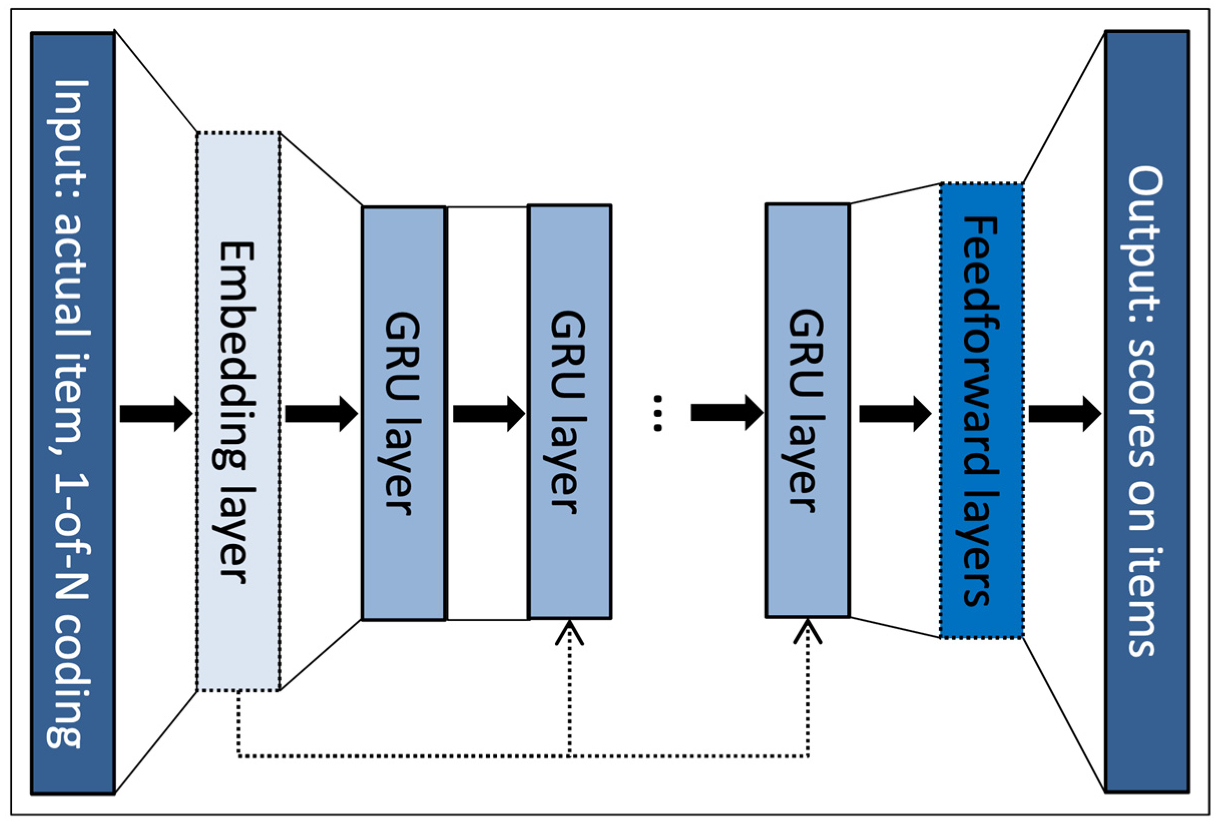
GRU4REC is among the earliest approaches in which recurrent neural networks are extensively utilized in session-based recommender systems and is broadly acknowledged as a robust benchmark model within this field. The architecture of GRU4REC is illustrated in Figure 1.

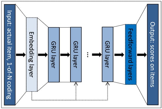
Figure 1. The GRU4REC network architecture [8].

The input embedding consists of one-hot representations of items.

The authors of GRU4REC expanded on their work in 2018, exploring various loss functions and reporting a 35% improvement in performance with the updated loss functions [14]. In this paper, we utilize the Bayesian Personalized Ranking (BPR) loss function.

BPR is a matrix factorization method that uses pairwise ranking loss; instead of comparing the score of a positive item with a single sampled negative item, it evaluates the score of the positive item against multiple sampled negative items and calculates the average of these comparisons to determine the loss [15]. The loss at a given point in one session is defined as

$$L_S=-{\displaystyle \frac{1}{N_S}}·\sum _{J=1}^{N_S}log(\sigma ({\widehat{r}}_{s,i}-{\widehat{r}}_{s,j}))$$

(5)

where $N_S$ is the sample size, ${\widehat{r}}_{s,k}$ is the score on item k at the given point in the session, i is the desired item, and j is the negative sample.

4. Experiments

4.1. Datasets

In our experimental setup, two e-commerce recommendation datasets are leveraged: Diginetica and RetailRocket. Both datasets are publicly available; Diginetica can be accessed via the CIKM Cup 2016 repository, and RetailRocket is obtainable from its official website. To introduce domain diversity, we also include the 30MU dataset, which contains music listening logs from Last.fm. The 30MU dataset is available for academic research via the Last.fm data portal. Detailed specifications and access information for these datasets are provided in Table 1.

Table 1. Data specifications of datasets.

Dataset	Diginetica	RetailRocket	30MU
Actions	264 k	210 k	640 k
Sessions	55 k	60 k	37 k
Items	32 k	32 k	91 k
Avg. Session Length	4.78	3.54	17.11

Compared to the additional two datasets, 30MU typically features a greater variety of items and sessions that are longer. Consistent with prior research, we exclude sessions containing only a single interaction and remove items with fewer than five interactions.

4.2. Stratified Dataset Evaluation

In our study, two stratification methods—target item propensity and historical item propensity—were selected to capture complementary aspects of recommendation bias. The target item propensity method directly reflects an item’s inherent popularity by considering its likelihood of being recommended, thereby serving as a clear metric for standalone exposure bias. In contrast, the historical item propensity method aggregates the popularity scores of items previously encountered in a session, offering valuable contextual insight into evolving user behavior. Together, these approaches provide a balanced evaluation framework that highlights both isolated popularity effects and the influence of session context on model performance. While alternatives such as median aggregation, weighted averages prioritizing recent interactions, or composite metrics that combine these insights could be considered, our experiments indicate that the dual approach effectively reveals the strengths and weaknesses of the recommendation models.

To identify whether such strata exist in session-based recommendation systems, which is the first objective, we adopt the evaluation approach detailed by Jadidinejad et al. [1]. Based on context-aware propensity, this method stratifies each action and calculates the propensity score for each item. By implementing this in session-based recommendation system datasets, we create two techniques for assigning a score to each action in a session. Through the use of these techniques, the evaluation data are divided into two subsets: Q1, which includes actions with low scores, and Q2, which includes actions with high scores.

• Stratification via the target item’s propensity: In this method, the propensity of the target item is directly adopted. However, in practice, our algorithm must not have access to the target item of an action until after the assessment of that action is finished. Therefore, while our approach is ideal, it somewhat violates the assessment procedure by revealing future data.
• Stratification according to the inclinations of historical items within the session: Instead of depending on information from the target item, we utilize data from all items that have been encountered earlier. A simple method of aggregating this information is by calculating the mean value of the propensity scores of the historical items within the session. Suppose this aggregated metric is correlated with the target item’s propensity. To illustrate this, Figure 2 demonstrates the empirical correlation between these metrics for each dataset.
  

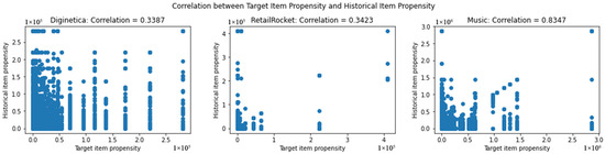  Figure 2. Relationship between the target item’s propensity and the mean propensity of historical items.

The 30MU dataset shows a strong correlation, while the two e-commerce datasets exhibit a low correlation.

4.3. Evaluation Metrics

To assess the performance of each model on the stratified test data, we adopt the evaluation metrics outlined in Ludewig et al. [2]. Our analysis highlights the key metrics outlined below; in these areas, neural network models are consistently outperformed by non-neural network models.

• HitRate (HR) assesses the fraction of instances where the model’s predicted item aligns with the target item.

  $$HR={\displaystyle \frac{\left|A_{hit}^L\right|}{\left|A_{all}\right|}}$$

  (6)
• The relevance of recommendations is assessed by Mean Reciprocal Rank (MRR) by computing the inverse rank of each recommended item and subsequently averaging this value across all actions.

  $$MRR={\displaystyle \frac{1}{\left|A_{all}\right|}}\sum _{u=1}^{\left|A_{all}\right|}RR(a)$$

  (7)

  $$RR=\sum _{i\le L}{\displaystyle \frac{{relevance}_i}{{rank}_i}}$$

  (8)

4.4. Training and Evaluation

In our experiments, SKNN was selected for the KNN-based model and GRU4REC was selected for the deep learning-based model. SKNN was chosen due to its long-standing popularity among practitioners, and GRU4REC due to it being one of the pioneering models in the field and frequently acting as a robust benchmark for novel neural network models. The Python 3.8 framework session-rec was the primary basis for our training and inference framework. However, we made several modifications, including the implementation of extra models based on propensity scores, inference scripts, and revisions to certain evaluation classes to better align with our evaluation objectives. The hyperparameters used for each model were primarily sourced from Ludewig et al.:

• For SKNN, set sample size = 500, cosine similarity, k = 100.
• For GRU4REC, Adagrad was employed as the learning algorithm; set the bpr-max loss function, momentum = 0.1, learning rate = 0.03, and dropout rate = 0.3 [6].

5. Results

5.1. Item Propensity Distribution

To better understand their characteristics, we begin by visualizing the item propensity for each dataset. Through the application of the power law algorithm independently to each dataset, the item propensity is determined through Equation (3). Furthermore, we display the logarithmic item propensity distribution of the three datasets in Figure 3.

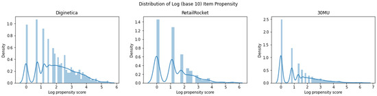
Figure 3. Distribution of item propensities across three datasets, displayed on a log scale (base 10).

Since the power law has been used, the scope of item propensity values is close across the datasets. However, the distributions for Diginetica and RetailRocket are more spread out, while the distribution for 30MU is predominantly clustered toward the lower end.

5.2. Evaluation Based on Propensity

The evaluation data are stratified by action-wise propensity and split into different proportions, and the results of various models on these strata are reported. Moreover, we compute the action-wise propensity score by employing the two methods outlined in Section 4.2. Then, we conduct experiments using different x values, where the x% percentile of the propensity score splits the entire evaluation dataset into two parts: Q1 and Q2. The performance of SKNN and GRU4REC is evaluated on both portions to investigate how each model handles actions with different propensities.

The results for Diginetica are presented in Figure 4 and Figure 5.

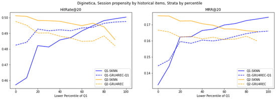
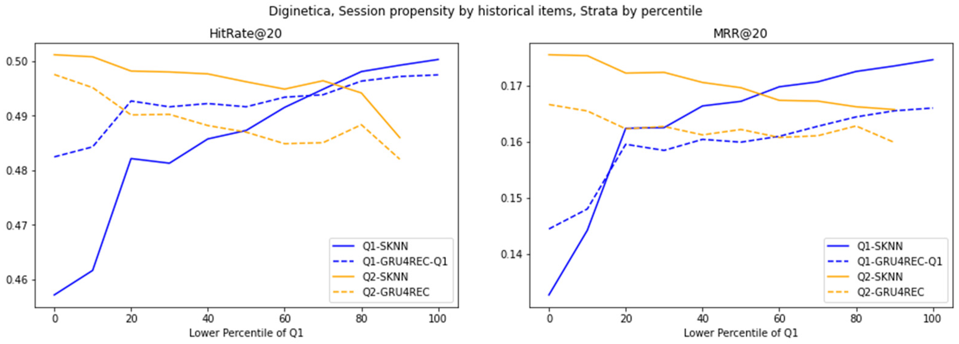
Figure 4. Evaluation of different models on Diginetica strata, stratified by percentile cutoffs, using the average propensity of historical items as the action-wise propensity.

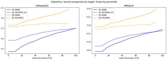
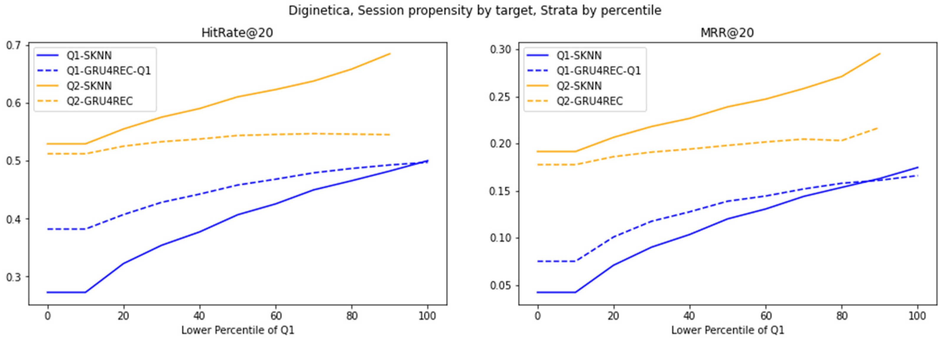
Figure 5. Evaluation of different models on Diginetica strata, stratified by percentile cutoffs, using the target item’s propensity as the action-wise propensity.

The architectural dichotomy between sequence models and frequency-based models drives their average historical trend performance. The RNN structure of GRU4REC has a good sparse interaction mechanism (Q1), which can capture potential temporal dependencies even in unpopular projects. In contrast, SKNN’s dependence on the frequency of project co-occurrence reduces performance differences in high-trend scenarios dominated by repetitive patterns (Q2). The advantages of GRU4REC gradually weaken, highlighting the specialization of long tail proposals, in sharp contrast to the practicality of SKNN in light distributions.

The trend of switching to the target project increases the advantage of GRU4REC (Q1) in low-trend scenarios and highlights the specificity of the scenario. GRU4REC alleviates the cold start problem of rare projects by directly modeling the dependencies of the target project in the sequence. However, the improvement in SKNN’s Q2 boundary narrowed the performance gap by aligning the frequency heuristic algorithm with user behavior, with high-trend projects dominating. This highlights how metric granularity interacts with model architecture.

The results for RetailRocket are shown in Figure 6 and Figure 7.

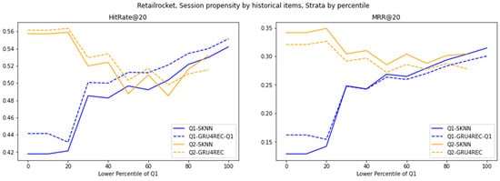
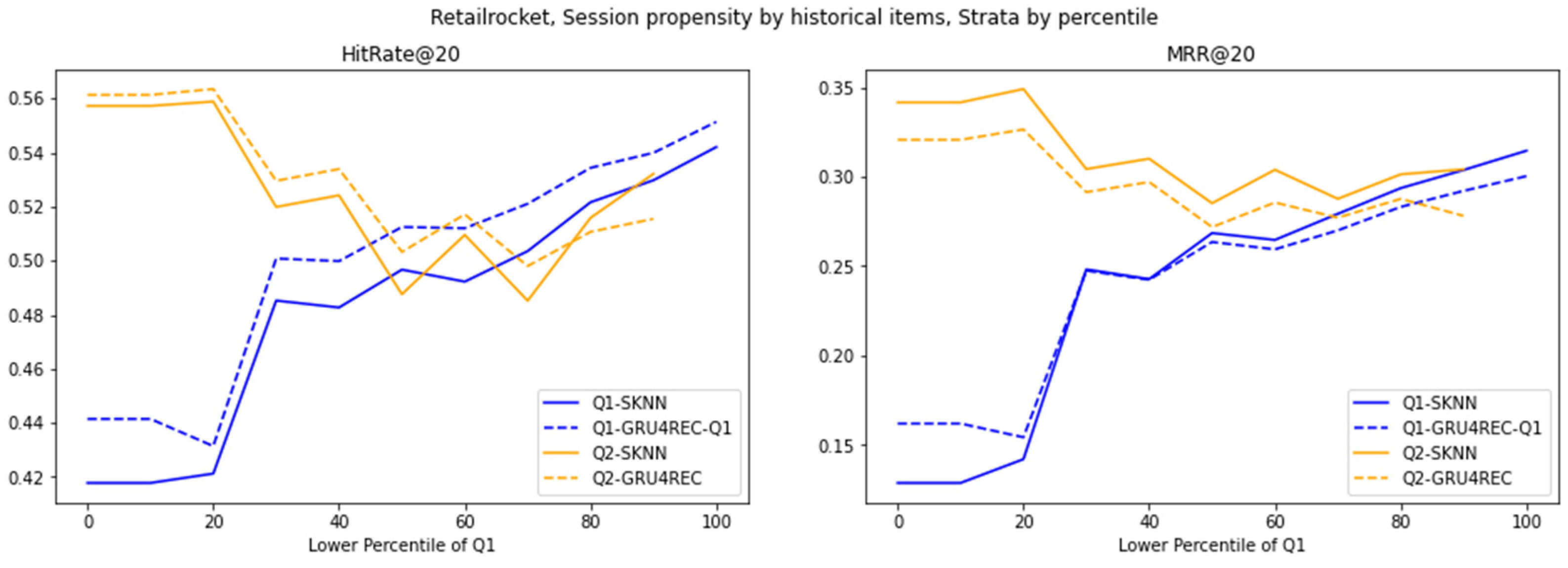
Figure 6. Evaluation of various models on the RetailRocket dataset, stratified by percentile cutoffs.

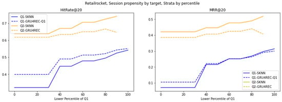
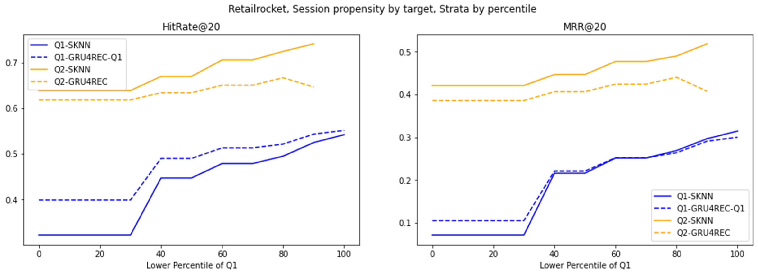
Figure 7. Performance of various models on the RetailRocket dataset, divided into strata based on percentile cutoffs.

The low variability in RetailRocket interaction reconstructed the motion of the model. In contrast to Diginetica, the G1 superiority of GRU4REC decreases. This is due to the lack of diversity that can be used in the homology and time modeling of datasets, even for distributed interactions. SKNN’s second-quarter competitive performance coincided with a high-trend repeating pattern for GRU4REC. A decrease in the rate of return at a high percentage of bits indicates the excessive fitting of redundant signals. This indicates how the dataset’s variability modulates the effectiveness of the model: GRU4REC develops actively in chaos, and SKNN actively develops in stable regimes.

RetailRocket’s temporal stability further moderates model divergence under target item propensity. GRU4REC’s smaller Q1 lead reflects consistent rare-item co-occurrences, enabling SKNN to approximate temporal patterns via frequency. SKNN’s Q2 resilience, paired with muted cross-strata variation, underscores its adaptability to predictable, high-propensity targets. Unlike Diginetica’s volatility, RetailRocket’s stability reduces the need for GRU4REC’s sequential complexity, favoring SKNN’s simplicity in static regimes.

The results for 30MU are shown in Figure 8 and Figure 9.

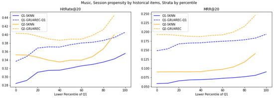
Figure 8. Evaluation of various models on strata of 30MU dataset, created using percentile cutoffs.

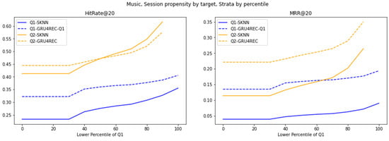
Figure 9. Performance of different models on strata of 30MU dataset, generated using percentile cutoffs.

Sparsity dictates model utility in average-propensity scenarios. GRU4REC’s Q1 dominance persists across percentiles, leveraging sequential generalization to overcome data scarcity. SKNN’s Q1 struggles and Q2 parity, however, reveal a critical threshold: high-propensity interactions exhibit pattern saturation, where frequency counting suffices. This bifurcation advocates context-aware hybridization—GRU4REC for sparse, evolving patterns and SKNN for dense, stable regimes.

30MU’s high user-behavior variance amplifies GRU4REC’s adaptability. Its significant Q1 lead stems from modeling erratic, rare-item interactions, while SKNN’s static heuristics falter in volatile environments. SKNN’s stable but inferior Q2 performance confirms its rigidity to behavioral shifts, contrasting with RetailRocket’s results. This divergence underscores that user-behavior variance, not just propensity, dictates model viability, advocating the use of GRU4REC for dynamic systems and SKNN for static ones.

This section presents the item propensity distribution for the Diginetica, RetailRocket, and 30MU datasets, as well as an analysis of model evaluation and ensemble effects based on propensity-based stratification. The propensity score distribution of the Diginetica dataset exhibits a typical power law pattern, where the majority of items have low popularity, while only a few popular items demonstrate significantly higher propensity scores. This distribution reflects the common popularity bias in e-commerce platforms. In contrast, the propensity score distribution of the 30MU dataset is more balanced, with most songs having relatively similar levels of popularity. This indicates exposure to a more diverse range of items in music recommendation systems, although there is still some bias against less popular songs. The evaluation results based on propensity-based stratification show that in the Diginetica dataset, GRU4REC significantly outperforms SKNN on low-popularity items, demonstrating its robustness in handling less popular items, whereas SKNN performs better on highly popular items. In the 30MU dataset, GRU4REC consistently performs better across all strata, highlighting its stability in capturing diverse user interests. Further analysis of model ensemble methods indicates that fixed-weight ensembles effectively combine the strengths of SKNN in recommending popular items and the robustness of GRU4REC for less popular items, thereby improving overall performance. Dynamic-weight ensembles, on the other hand, dynamically adjust weights in real time based on propensity scores, further optimizing recommendation results and achieving outstanding performance, especially in recommending less popular items.

Overall, these findings underline the importance of propensity-based stratification and ensemble methods in improving recommendation system performance.

6. Discussion

For the e-commerce datasets (RetailRocket and Diginetica), when the percentile decreases—indicating a drop in the average popularity of items—GRU4REC significantly outperforms SKNN. In contrast, no such trend is observed in the 30MU dataset, where the difference in performance between the two models is stable across various x values.

Furthermore, we investigate the correlation between the two stratification methods presented in Figure 2. The 30MU dataset exhibits a strong correlation, whereas the e-commerce datasets show weaker correlations. However, this correlation does not appear to influence the experimental results. Even with regard to 30MU, the trends depicted in the line plots in Figure 8 and Figure 9 differ between the two stratification methods.

To assess the reliability of deep learning models in dealing with unpopular items, two subsets are defined: S1, containing the actions of the minimum 10% propensity scores, and S2, comprising actions with the maximum 10% propensity scores. Afterward, the performance of both models on these subsets is evaluated and the ratio of the score for S1 to the score for S2 is calculated. The results are presented in Table 2:

Table 2. Results for the ratios between the two models.

Dataset	Metric	SKNN	GRU4REC
DIGINETICA	HitRate@20	0.3978	0.7007
	MRR@20	0.1424	0.3455
RetailRocket	HitRate@20	0.4351	0.6175
	MRR@20	0.1383	0.2589
30MU	HitRate@20	0.7293	0.7803
	MRR@20	0.4187	0.6241

This table shows that GRU4REC consistently achieves high performance across all datasets, as its ratios are higher when compared to those of SKNN. This indicates that GRU4REC demonstrates greater robustness when dealing with unpopular items.

Given the observed trend in which GRU4REC outperforms SKNN on actions related to lower propensity scores, while SKNN outperforms GRU4REC on actions with higher propensity scores, a model ensemble approach is explored, guided by action-wise propensity during evaluation. For this purpose, the method we use is a stratification technique grounded in the historical item propensities within the session, as outlined in Section 4.2.

6.1. Ensemble Methods Based on Fixed Weight

We determine a dataset-specific threshold for each action based on the distribution of action-wise propensity scores. Prediction scores from GRU4REC and SKNN are then weighted and combined to produce the conclusive prediction score attributed to an action. Threshold and weights serve as hyperparameters; with a symmetrical weighting strategy applied, SKNN and GRU4REC obtain reversed weights within the two strata.

This method demonstrates significant advantages on e-commerce datasets, achieving a 10% relative improvement in HitRate@20 on Diginetica and a 6% improvement on RetailRocket. Notably, the performance gains are robust and not highly sensitive to the choice of weights. For the 30MU dataset, while GRU4REC consistently outperforms SKNN across all strata, incorporating SKNN’s predictions in the ensemble still yields additional improvements.

6.2. Ensemble Methods Based on Dynamic Weight

In the prior method, fixed weights for different models across distinct propensity strata are used. In this setup, all actions within the same stratum are assigned the same set of ensemble weights, regardless of their propensity scores. To address this limitation, our proposed dynamic-weight ensemble technique computes the weights for each action dynamically, depending on its specific propensity score. This ensures that the weights assigned to each action are more accurately aligned with its propensity. The weights ${\omega }_1$ and ${\omega }_2$ are calculated using the following formula, where the propensity score of action i is denoted as $p_i$:

$$p_{normalized,i}={\displaystyle \frac{log(p_i+{10}^{-9})-{\widehat{p}}_{mean}}{{\widehat{p}}_{std}}}$$

(9)

$${\omega }_1={\displaystyle \frac{1}{1+e^{p_{normalized,i}+\alpha }}},{\omega }_2=1-{\omega }_1$$

(10)

The formula applies a sigmoid transformation that is shifted by x to the negative of the log-normalized propensity score. Since the sigmoid function is a smooth, bounded (0–1) transformation, it is ideal for mapping propensity scores to ensemble weights. Its S-shaped curve enables gradual weight transitions, contrasting fixed strata boundaries, preserving nuanced differences between actions. The key hyperparameters involved are $\mathsf{\alpha }$, mean, and standard deviation (std). The mean and std are approximate measures of the average of and variability in actions across the entire test dataset. These values could be estimated by implementing actions based on the training set, as there is a complete overlap in items between the two datasets. The parameter $\mathsf{\alpha }$ controls the horizontal shift of the sigmoid function and is fine-tuned through grid search.

The 10% percentile threshold T is set at 12.425 for Diginetica, 1.000 for RetailRocket, and 110.085 for 30MU. The parameter ${\omega }_2$ represents the weight allocated to GRU4REC model predictions for low-propensity actions, while simultaneously serving as the weight for the SKNN model’s predictions for actions with high propensity. The result for comparison is shown in Table 3.

Table 3. Evaluation results in the model ensemble scenario and single-model evaluation.

Dataset	Metric	SKNN	GRU4REC	1.0	0.9	0.8	0.7	0.5	0.2 1
DIGINETICA	HitRate@20	0.500	0.497	0.504	0.548	0.553 2	0.550	0.540	0.520
	MRR@20	0.175	0.166	0.175	0.183	0.186	0.187	0.188	0.180
RetailRocket	HitRate@20	0.548	0.551	0.550	0.581	0.581	0.578	0.577	0.565
	MRR@20	0.311	0.300	0.320	0.326	0.326	0.325	0.323	0.310
30MU	HitRate@20	0.355	0.4057	-	-	0.420	-	-	-
	MRR@20	0.09	0.194	-	-	0.160	-	-	-

¹ Ensemble, weight ${\omega }_2$. ² Best performance across compared methods.

The performance outcomes are presented in Table 4.

Table 4. Comparison of results between the fixed-weight ensemble approach and the dynamic-weight ensemble approach.

Dataset	Metric	Ensemble, Dynamic Weight	1.0	0.8	0.5 1
DIGINETICA	HitRate@20	0.556 2	0.504	0.553	0.520
	MRR@20	0.186	0.175	0.186	0.180
RetailRocket	HitRate@20	0.586	0.550	0.581	0.565
	MRR@20	0.324	0.320	0.326	0.310

¹ Ensemble, fixed weight ${\omega }_2$. ² Best performance across compared methods.

The dynamic-weight method is analyzed in comparison with three fixed-weight ensemble methods. While it achieves the highest HitRate of all approaches, the MRR metric improvement is less pronounced.

To effectively apply the dynamic-weight ensemble method, practitioners should first preprocess historical interaction data to compute propensity scores for each action, normalize user–item interactions, and estimate the likelihood of item exposure.

Then, implement the dynamic weighting strategy by applying a sigmoid transformation to the normalized propensity scores, compute weights for each action using the formula in Section 6.2, and fine-tune key hyperparameters such as the horizontal shift, mean, and standard deviation via grid search or cross-validation. Next, combine predictions from base models (e.g., GRU4REC and SKNN) using the dynamically computed weights, designing this integration to allow real-time computation for prompt adaptation to incoming data and changing user behavior.

After that, validate the ensemble model on a hold-out dataset to ensure consistent and statistically significant performance improvements, and once the model is deployed, continuously monitor evaluation metrics like HitRate and MRR, with regular hyperparameter updates as user preferences evolve.

Finally, considering the additional computation involved in dynamic-weight ensembles, assess the trade-off between accuracy gains and computational overhead, and explore distributed computing solutions or efficient online updating mechanisms to scale the dynamic-weight computation process in production environments. By following these guidelines, practitioners can integrate dynamic-weight ensemble methods into real-world recommendation systems, balancing improved accuracy with practical runtime efficiency.

7. Conclusions

This study investigated the impact of deviation on recommendation systems by comparing the performance of SKNN and GRU4REC across three datasets (Diginetica, RetailRocket, and 30MU) using a propensity evaluation threshold, revealing that GRU4REC excels at recommending less popular items in e-commerce while SKNN performs well with mainstream products, with GRU4REC outperforming SKNN on fashion datasets and the music dataset showing a correlation between user interaction history and item prominence. This work contributes a hierarchical evaluation framework with trend-based propensity scoring, novel fixed-weight and dynamic-weight ensemble methods integrating the strengths of SKNN and GRU4REC, and a paradigm shift reframing bias as a contextual feature to balance recommendation accuracy and diversity. However, limitations include the narrow scope of datasets and scalability concerns with the dynamic-weight ensemble method. Future research should test the methods in broader domains (news, social media), analyze runtime and scalability, and refine ensemble strategies to bridge the gap between theoretical and practical recommendation system implementations.

References

- Jadidinejad, A.H.; Macdonald, C.; Ounis, I. The Simpson’s paradox in the offline evaluation of recommendation systems. ACM Trans. Inf. Syst. (TOIS) 2021, 40, 1–22. [Google Scholar] [CrossRef]
- Ludewig, M.; Mauro, N.; Latifi, S.; Jannach, D. Empirical analysis of session-based recommendation algorithms. User Model. User-Adapt. Interact. 2020, 31, 149–181. [Google Scholar] [CrossRef]
- Maurício, J.; Domingues, I.; Bernardino, J. Comparing Vision Transformers and Convolutional Neural Networks for Image Classification: A Literature Review. Appl. Sci. 2023, 13, 5521. [Google Scholar] [CrossRef]
- Saadatfar, H.; Khosravi, S.; Joloudari, J.H.; Mosavi, A.; Shamshirband, S. A New K-Nearest Neighbors Classifier for Big Data Based on Efficient Data Pruning. Mathematics 2020, 8, 286. [Google Scholar] [CrossRef]
- Jannach, D.; Ludewig, M.; Lerche, L. Session-based item recommendation in e-commerce: On short-term intents, reminders, trends, and discounts. User Model. User-Adapt. Interact. 2017, 27, 351–392. [Google Scholar] [CrossRef]
- Wang, H.; Du, Y.; Jin, C.; Li, Y.; Wang, Y.; Sun, T.; Qin, P.; Fan, C. GACE: Learning graph-based cross-page ads embedding for click-through rate prediction. In Neural Information Processing; Springer Nature: Singapore, 2024; pp. 429–443. [Google Scholar] [CrossRef]
- Ludewig, M.; Jannach, D. Evaluation of session-based recommendation algorithms. arXiv 2018, arXiv:1803.09587. [Google Scholar] [CrossRef]
- Hidasi, B.; Karatzoglou, A.; Baltrunas, L.; Tikk, D. Session-based recommendations with recurrent neural networks. arXiv 2016, arXiv:1511.06939. [Google Scholar] [CrossRef]
- Li, J.; Ren, P.; Chen, Z.; Ren, Z.; Ma, J. Neural attentive session-based recommendation. arXiv 2017, arXiv:1711.04725. [Google Scholar] [CrossRef]
- Wu, S.; Tang, Y.; Zhu, Y.; Wang, L.; Xie, X.; Tan, T. Session-based recommendation with graph neural networks. In Proceedings of the AAAI Conference on Artificial Intelligence, Honolulu, HI, USA, 27 January–1 February 2019; Volume 33, pp. 346–353. [Google Scholar] [CrossRef]
- Schnabel, T.; Swaminathan, A.; Singh, A.; Chandak, N.; Joachims, T. Recommendations as treatments: Debiasing learning and evaluation. arXiv 2016, arXiv:1602.05352. [Google Scholar] [CrossRef]
- Yang, L.; Cui, Y.; Xuan, Y.; Wang, C.; Belongie, S.J.; Estrin, D. Unbiased offline recommender evaluation for missing-not-at-random implicit feedback. In Proceedings of the 12th ACM Conference on Recommender Systems, Vancouver, BC, Canada, 2 October 2018. [Google Scholar] [CrossRef]
- Steck, H. Item popularity and recommendation accuracy. In Proceedings of the Fifth ACM Conference on Recommender Systems, RecSys 11, Chicago, IL, USA, 23–27 October 2011; pp. 125–132. [Google Scholar] [CrossRef]
- Hidasi, B.; Karatzoglou, A. Recurrent neural networks with top-k gains for session-based recommendations. In Proceedings of the 27th ACM International Conference on Information and Knowledge Management, Torino, Italy, 22–26 October 2018; pp. 843–852. [Google Scholar] [CrossRef]
- Rendle, S.; Freudenthaler, C.; Gantner, Z.; Schmidt-Thieme, L. BPR: Bayesian personalized ranking from implicit feedback. In Proceedings of the UAI’09: 25th Conference on Uncertainty in Artificial Intelligence, Montreal, QC, Canada, 18–21 June 2009; pp. 452–461. [Google Scholar]
Disclaimer/Publisher’s Note: The statements, opinions and data contained in all publications are solely those of the individual author(s) and contributor(s) and not of MDPI and/or the editor(s). MDPI and/or the editor(s) disclaim responsibility for any injury to people or property resulting from any ideas, methods, instructions or products referred to in the content. |
© 2025 by the authors. Licensee MDPI, Basel, Switzerland. This article is an open access article distributed under the terms and conditions of the Creative Commons Attribution (CC BY) license (https://creativecommons.org/licenses/by/4.0/).