Abstract
The change-point model is an established methodology for the construction of self-starting control charts. Change-point charts are often nonparametric in order to be independent from any specific assumptions about the process distribution. Nonetheless, this methodology is usually implemented by considering all possible splits of a given stream of observations into two adjacent sub-samples. This can make the recent observations too influential and the chart’s signals too dependent on limited evidence. This paper proposes to correct such a distortion by using a window approach, which forces the use of only comparisons based on sub-samples of the same size. The resulting charts are “omnibus”, with respect to their having any kind of shift and also any direction of such shifts. To prove this, this paper focuses on a chart based on the Cramér–von Mises test. We report a simulation study evaluating the average number of readings to obtain a signal after a known shift has occurred. We conclude that, beyond being stable with respect to the direction of the shift, the new chart overcomes its competitors when the distribution heads toward regularity. Finally, the new approach is shown to have successful application to a real problem about air quality.
Keywords:
statistical process monitoring; self-starting control charts; nonparametric control charts; change-point model; window approach; Monte Carlo simulations; air quality data MSC:
62P30
1. Introduction
Control charts are a known statistical tool aimed at finding empirical evidence that a process quality, as measured by a univariate characteristic, has shifted from the usual in-control (IC) status to a situation of anomalous variability denoted as an out-of-control (OC) condition (for the sake of clarity, all the abbreviations are listed at the end of the paper). Two classical references for control charts are [1,2].
Starting from these books, many authors have emphasized that a wider application of charting techniques to a variety of control problems requires the relaxation of the classical rigid assumptions. For instance, [3] recently used a dataset about a hard-baking process, reported in [1], as a motivating example: they showed that a key quality characteristic of the process could hardly fit the usual normal assumption. The same example emphasized the need for tools able to detect many different kinds of change in the process distribution. Other relevant examples are reported by [4,5,6].
In the last decades, control charts have been implemented in different areas, such as medical condition monitoring, climate change detection, speech recognition, image analysis, human activity analysis, etc. Thus, many similar examples can be found of the need to go well beyond the normal distribution. In addition, it is clear that shifts from the IC situation may not involve just location and scale but also other general aspects of the shape. Furthermore, such shifts do not necessarily head toward an irregular shape; they may even go in the opposite direction. For instance, in the example reported in Section 4 we will consider some environmental variables that showed a sudden drift toward a more (statistically) regular distribution. Incidentally, it can be noted that control charts are increasingly being used for the analysis of environmental data in recent years (see, among others, [7]).
It is clear that many of the needs outlined above can be met by reverting to nonparametric charts (see [2,8,9,10]). However, we think that further improvement can be obtained by combining the use of nonparametric tools with a new implementation of the change-point (CP) methodology, as specified in the following discussion. We anticipate here that the new implementation is, actually, the true key to providing charts with substantial power with respect to a large variety of shifts in the distribution.
The CP model was introduced as a new approach to build control charts in a pioneering work by [11]. More specifically, the CP model hypothesizes the existence of an unknown time point, , in the stream of available observations such that are independent and identically distributed (iid) variables according to while are iid according to a different model The chart has then the two-fold task of establishing whether and of estimating the value of in the affirmative case.
Depending on the assumptions made on and many statistical tests to reject the homogeneity of the two samples and can be used. However, the problem is made difficult by the indeterminacy of . Ref. [11] showed that, under the assumption that
(all parameters being unknown), a generalized likelihood-ratio test can be implemented as follows. First, given all putative change points two sample means are computed as and and the common variance is estimated by Second, the usual two-sample t statistic is considered
Third, the maximum absolute value of (2) is taken over all the possible splits of the n observations into two adjacent non-empty sets:
Of course, a chart produces an OC signal whenever for a suitable threshold value which depends on the current sample size. Jointly, an estimate of the change point is obtained by retracing the split that gave the maximum value for the signal, that is, by setting
Regardless of its characterization as a generalized likelihood test, the procedure based on (3) can be considered as a natural implementation of the CP methodology. Indeed, when the assumptions in (1) are modified, one can simply think to substitute (2) with any suitable two-sample test statistic and to compute a maximum value over all possible splits of the current dataset, like in (3), provided that the arguments are made comparable. As discussed below, the literature reports many applications of this classical implementation, so that potentially any kind of shift in the process characteristics can be managed.
Notice that even if the CP methodology can be usefully applied for Phase I control problems (see [12]), its nature intrinsically prevents any conceptual distinction between phases of control. Indeed, in a Phase I analysis, a fixed sample size is usually considered to establish whether the current set of data is as “clean” as necessary to provide reliable estimates of the IC distribution’s characteristics. However, as seen, the CP methodology does not need to compare such characteristics with those observed in a hypothetical Phase II study. Thus, control can start without a preliminary adjustment of the chart or, to use popular terminology, the latter can be a self-starting chart.
In this paper, we will concentrate on such applications where the available readings can be considered as continuously increasing streams of data. At each step of a self-starting procedure, all the currently gathered observations are used to detect possible shifts in the process. In any case, a suitable amount of initial data must be provided to obtain effective control. That happens because of the need of the chart to obtain sufficient knowledge of the underlying process but also for computational purposes (for instance, (2) needs at least three observations).
The b observations needed to start control must be obtained under stable conditions for the process. They are, in a sense, “burnt” because, even if the change point can be estimated as belonging to them, the chart can only signal after all of the change points are gathered. Theoretically, the size b of this burning-out set depends on the assumptions made on the process and on the test statistic applied but, in essence, it is a question of a subjective choice. Some general indications are found in the literature (see, for instance, [13]). One must consider, for instance, that a different set of threshold values is to be determined for every fixed , as detailed in the following. Thus, it is a common practice to apply just some conventional values for like those used to build the tables reported in the Appendix A.
To get into details, let us go back to the proposal by [11]. Consider first the threshold value to be used when the control has just started, that is, when observations are available. Even if for every fixed the statistic (2) has a manageable distribution under the null hypothesis () that (or equivalently, that ), the null distribution of (3) is analytically intractable. Thus, Ref. [11] proposed to revert to simulations to determine Such a value is based on the following marginal probability statement:
where denotes the desired false-alarm rate. Different problems arise for the successive values in the sequence of the thresholds Indeed, when one needs to consider some suitable conditional probabilities. The aim is still to guarantee the fixed rate for all steps of control by setting
Operatively, a large number (say, M) of sequences of readings are randomly drawn under the assumption made when the process is IC. The vector of statistics is computed for every simulated sequence. As a first step, the resulting empirical distribution of is used to determine its percentile of order ; such a value is set for Then, the simulated sequences for which are discarded and the empirical distribution of is computed just upon the remaining sequences. Such a distribution is used to determine a new percentile, still of the order , which is set for Further simulated sequences are discarded consistently, the value of is determined, and the procedure goes on like this until the value of is obtained.
The obvious limitation is that, as the procedure moves forward, the last threshold values may be computed on the basis of too few simulated sequences. Specifically, the total frequency of the empirical distribution of is only equal to This figure, for instance, can be as low as 98,884 when , , and even if sequences are used at the start. Recall that, for each simulated sequence, the procedure needs to divide all the possible splits of the current n observations into two adjacent sets. This fact is likely to burden the computational effort. Thus, the value of M cannot be indefinitely raised unless a method to reduce the number of splits is found.
The positive effect is that, as n grows, the actual value taken by tends to stabilize. Even in [11], then, the existence of some empirical approximating rules has been underlined. We think that the simplest rule is just to set for all for a suitable value Such a rule is equivalent to claim that, after a warming-up period of w new readings, the chart reaches stability, so the mathematical condition to generate a signal can be made uniform. Of course, despite all approximations, the final aim is still to assure the targeted false-alarm rate or, maybe more effectively, the desired level for its reciprocal, the IC average run length (IC-ARL). Thus, the ability to meet this goal should be taken into due consideration when different implementations of the CP methodology are compared.
Looking at the (conditional) null distribution of can reveal other interesting elements for discussion. Consider, for instance, a chart based on (1)–(3) and set Moreover, recall that the estimation of the change point can be achieved after a signal is produced by the chart, so it is sensible to simulate the following expected value . On the basis of replicates, that value is reported in Table 1, for and for some commonly used values of the false-alarm rate: One can notice that when the control starts, is obviously estimated as the center of the ten available observations. Thus, on average, a (false) signal is produced on the basis of the split of such observations into two balanced samples. While the estimate of coherently increases with however, it also interestingly departs from as n grows. This means that even when the process has not shifted from the IC situation, the chart tends to favor unbalanced samples for its judgment.

From a different point of view, Table 1 underlines that the chart tends to judge the recent observations as more “informative” than the old ones. Sometimes this can be a serious drawback, according to two considerations. First, even when the process is IC, the occurrence of outliers in the ongoing stream may influence the chart too strongly. Indeed, such deviating data are likely to belong to a small sample, where few ordinary observations are available to “compensate” for them. Second, when the process is truly OC, the power of the chart is likely to be reduced by the predominant use of unbalanced samples. Look, for instance, at Table 2, where the powers of the simple t test are reported, when a total set of 20 observations is differently partitioned into two samples (see the caption for the computational details); as known, the highest value is obtained for balanced samples and the power decreases with the extent of disbalance.
Table 2.
Powers of the two-sample 5% test for the equality of the means of two normal homoskedastic populations. Computations are made for , and when the total size 20 is differently partitioned into two samples of sizes and .
The motivations above justify the evaluation of possible modifications of the CP methodology. As detailed in the following section, we will try both to reduce the number of comparisons needed to compute the charting statistic and to force the use of balanced samples for such comparisons. The same section will also discuss the implementation of a proposed modification and the determination of the threshold values of a related control chart. Section 3 will present a simulation study aimed at comparing different approaches towards build a chart based on the CP model. Section 4 will provide an application of the newly proposed chart to monitor the quality of air. Section 5 will draw some conclusions.
2. New Methodology and Its Implementation
Before getting into details, some notes about the sketched generalization of (2) and (3) in using different test statistics are reported and the related notation is updated.
Clearly, any two-sample statistic can be substituted to (2), even if the maximum computed in (3) does not need to be influenced by the value taken by Indeed, notice that under the hypothesis that both and are iid according to has a t distribution with degrees of freedom, which means that its expectation and variance do not depend on That makes it sensible to use (3) to compare competing splits of the total set of observations into two samples. Equivalently, does not need to be standardized before the maximum over j is computed.
When a different test statistic is substituted to (2), however, its moments are likely to depend on i.e., on the individual sizes of the two samples. For instance, a natural extension of the t test is the Mann–Whitney statistic,
(where , provided that a is less than, equal to, or greater than zero, respectively). One may think of using (4) for such cases where normality cannot be assumed and a location shift of the process is suspected (see [13]). Thus, under the IC situation, the ’s are just independent variables with a common (continuous) distribution. Correspondingly, it is known that the expectation of is zero but its variance depends on j and equals As a consequence, to compare competing values of (i.e., those related to different splits of the dataset into two samples), one needs to standardize them. See [13] for further details.
Now, let us introduce a more general notation for the possible implementations of the CP methodology. Given the usual stream of n readings, denote by and two adjacent sub-samples; they are built to have size l and m, respectively, and the second sub-sample always includes the last reading Thus,
Consider a statistic
built to reject the homogeneity of the two sub-samples above. Denote by and , respectively, the expectation and the variance of under the hypothesis that all variables in are equally distributed. The definition of the charting statistic in (3) can be generalized as follows:
Clearly, the implementation and the performance of a chart based on depend on the suitability of the test statistic in (6) with respect to the control problem in hand and to the assumptions made on the process. The literature has extensively covered such an issue by proposing many alternatives to the original two-sample t statistic (see [13,14,15,16], to cite a few). Specifically, Ref. [16] used the Kolmogorov–Smirnov and the Cramér–von Mises test statistics.
In this paper, we will concentrate not just on the possible variation of (6) but on a modification of the methodology itself, namely, on an alternative to (7). To provide a fair comparison with the classical implementation of the CP methodology, we will always keep the same choice for (6). Specifically, we will not make any assumptions about the process (except for continuity) and always make use of the Cramér–von Mises statistic. This implies the setting of
where for every real and , we denote the empirical distribution functions of the two sub-samples in (5) and consider as the indicator function on the set
Notice that when (8) is used to implement (7), one of the two proposals in [16] is obtained. As anticipated above, Ref. [16] used both the Kolmogorov–Smirnov and the Cramér–von Mises tests to build two self-starting CP charts. The application of the former statistic, however, is made difficult by the non-existence of closed forms for and in this case. To solve this problem, Ref. [16] reverted to the observed asymptotic p-value in order to define the arguments of the maximum in (7). Without going into detail, we point out that some alternative solutions can be also provided. For instance, one may think of approximating the values of and using simulations for every fixed l and However, we prefer to avoid any further element of uncertainty, and thus we focus here on a statistic that can be easily standardized. When the choice in (8) is made, the following formulas can indeed be proven (see [17]):
Consider now Figure 1, which depicts the scheme followed in the classical implementation of the CP methodology, as described in the Introduction and in the lines above. The sequence of shapes represents a stream of readings available at a generic step of control. The last element is drawn as a circle to emphasize that it represents the latest observation added to the stream. The classical implementation considers all the possible splits of the stream into two adjacent sub-samples, which are represented by different colors. Every pair of sub-samples are compared and such comparisons are used to compute a maximum value, the charting statistic.
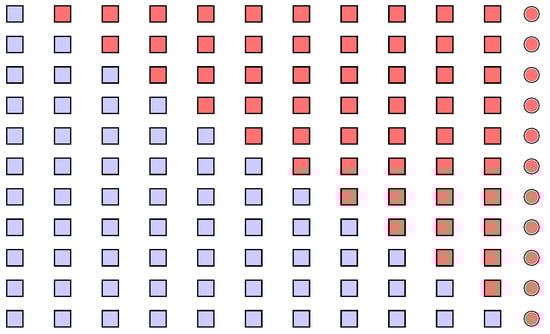
Figure 1.
Scheme of the classical implementation of the CP methodology: a stream of readings is represented by a sequence of shapes, where the circle represents the latest added observation; the considered splits into two sub-samples are highlighted by different colors.
One can easily notice that many comparisons are actually based on splits where the latest observation is potentially too influential. That observation, indeed, often belongs to a very small sub-sample, which means that it can be hardly compensated by other “common” readings. Even the first sub-sample, in effect, can be characterized by its small size. This is likely not to be a real problem, however, because this sample gathers mainly old readings, which are potentially drawn from the IC distribution.
To obtain effective control, a chart should provide prompt signals; however, it should be also protected against signals based on too limited evidence. In the case of the CP methodology, then, a conservative option is to ensure that each comparison between pairs of a sub-sample is as fair as possible. More specifically, one should contrast every sub-sample containing the latest observation only with sub-samples of the same size.
An application of this simple idea is depicted in Figure 2. Starting from a (hypothetical) comparison of two single observations, one can build consecutive pairs that are made just of balanced sub-samples. Under this scheme, all observations in the stream are used for control and the latest reading is still predominant enough to produce a signal. However, its role is tempered by a sufficient number of alternative observations. Conversely, the old readings (of which the very first is neglected just in the case there is an odd total size) are mainly used as a basis for comparison. This is consistent with the usual framework of self-starting charts, where control is supposed to start after a number of stable observations is collected.
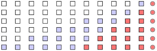
Figure 2.
Scheme of a proposed modification of the CP methodology, which is different from Figure 1 as just pairs of balanced sub-samples are considered.
The scheme proposed in Figure 2 can be formalized by a suitable modification of the charting statistic in (7). For a given choice of (6), one may substitute with
where denotes the integer part of Notice that for each the arguments in the maximum of (9) define a sort of “window” inspecting the last part of the stream. The width of such a window is progressively increased to cover the whole set of observations, so that (9) can be labeled as a dynamic window approach, in contrast to the split approach characterizing (7).
One may also think of possible simplifications of (9). For instance, the width of the window could be kept constant to a value : this can be denoted as fixed window approach. Another option could be a width that is progressively increased but just until a limit value is reached (constrained window approach). Despite the possible simplification, it is immediately clear that the implementation of these two alternative approaches is problematic. Indeed, the values of and must be arbitrarily chosen from 1 to without any possible guidance. The inadequacy of the fixed window and the constrained window approaches will be further highlighted in the last part of this section. Thus, operatively, one must be already satisfied with the simplification provided by the dynamic window approach because, with respect to (7), (9) reduces the number of arguments from to
The rest of this section is focused on the determination of the threshold values needed to build a chart based on the CP model. As outlined in Section 1 for the split approach, such a task is the major cause of computational burden when a chart is implemented. Clearly, the same simulation procedure described for the split approach can be applied to the window approach. With this aim, we wrote an elementary MATLAB code, which can easily reproduced. In addition, we decided to report in the Appendix A some of the results obtained. Obviously, the procedure can be customized according to one’s specific needs. Nonetheless, as detailed below, the settings used in the tables of the Appendix A can be a useful reference for many practical applications.
The Appendix A reports the simulated threshold values for a chart based on (8) and (9) with a burning-out set of b observations. Table A1, Table A2 and Table A3 are for , respectively, and Table A4 is set for and , and Table A5 for and All tables are based on simulated samples and built for six levels of the false alarm rate: , and
The main difficulty in the generation of threshold values rests in the computation time, especially when the sample size n is large. In this sense, a crucial choice is the number b of observations in the burning-out set or, equivalently, the size of the sample when control starts. As outlined in Section 1, different values of b need differently generated threshold values. Nonetheless, the values used in Table A1, Table A2, Table A3, Table A4 and Table A5 are easily adapted to many common applications. In addition, the tables are built for a large variety of possible values of the false-alarm rate The reciprocals of those values correspond to the levels commonly set for the IC-ARL, that is, the expected number of readings after which the chart produces a false signal.
A question remains regarding the last value of the sample size n characterizing each table in the Appendix A. It is not worthwhile to generate threshold values when n is too distant from the size at which control started. Indeed, the threshold values tend to stabilize very fast as n increases, and that is clear when looking at the final rows of the tables. As discussed in the Introduction, this fact gives room to possible approximations of the threshold values. Recall that an option is to apply a uniform condition for signals after a warming-up period. Specifically, given a constant w, one can complete the sequence of the threshold ’s by setting for every Of course, that rule proves to be operatively useful, but only if the value w is not too high. We suggest that it be set at about the half of the size used to start control.
Clearly, the efficacy of the approximating rule described above should be tested. In a sense, this is even a way to understand if the competing approaches to implement the CP model are indeed practically convenient. Thus, we conducted a dedicated simulation study to check if the targeted level of the IC-ARL can be guaranteed even if the sequence of threshold values is approximated. Some results are reported in Table 3. Specifically, the table considers two common levels of the false-alarm rate, and which correspond to a nominal IC-ARL (denoted ) of 20 and 100, respectively. Two cases are also considered for the size of the sample when control starts and for each of them some values of the warming-up constant are tested: the top part of the table considers with while the bottom considers and
Table 3.
Estimated IC-ARL when the thresholds are kept fixed to the last value for all (19 observations in the burning-out set) (top of the table) and (49 observations in the burning-out set) (bottom of the table).
Each figure in Table 3 was determined as an average over new samples that were randomly drawn in the IC situation. Each generated sample was passed to a chart whose threshold values had been predetermined and for which the approximation above had been applied. For each sample, the number of readings needed after the start to obtain a signal was recorded. The listed values can thus be considered as a sound estimate of the actual IC-ARL.
Table 3 reports results for the two main approaches considered: the split (SP) approach and the dynamic window (DW) approach. Further, the table gives some insight of the two simplifications discussed above, namely, the fixed window approach (FW) and constrained window approach (CW). For the sake of brevity, the table reports just the results obtained when the related exogenous constants were fixed as and . Different values of such constants were also tried, but the conclusions drawn are essentially confirmed.
One may argue that the targeted level of the IC-ARL is substantially reached after a warming-up of approximately half of the burning-out set, as anticipated above. That can be claimed for both the competing implementations of the CP methodology, the SP and DW approaches. There are situations where the SP approach is slightly more conservative than the DW approach. This might depend not just on the applied approximation but on the fact that the null distribution gives a non-negligible probability mass to single values, so the related distribution function is not strictly increasing everywhere.
Despite the possible simplifications introduced by the FW and CW, Table 3 shows that such approaches can hardly guarantee the targeted IC-ARL. This happens when w gets high values as well, i.e., even under a mild approximation of the real threshold values. This fact sums to the undesired need to fix the values of and exogenously, as discussed. In addition, some further unreported simulations showed that the FW and CW also have a poor performance under several OC situations. It means that they are scarcely competitive with respect to the proposed DW approach. Thus, in the following, we will concentrate just on the latter as an alternative to the classical implementation of the CP methodology.
Specifically, to add other elements of judgment, the next sections will investigate both DW’s ability to provide a prompt signal to given situations of shift from the IC distribution and its application to real data.
3. Simulation Study
We are now ready to evaluate the possible improvements of the CP methodology, thanks to the introduction of the DW approach. Our comparison will be limited to the nonparametric setting. Thus, all considered charts will be thought of as tools to detect any kind of shift from the IC distribution. As anticipated, we will use the Cramér–von Mises statistic reported in (8). In this sense, our study can easily be paralleled with that provided by [16], where just the SP approach is considered. Notice that the strengths of the DW approach could possibly be improved by even reverting to statistics other than (8). However, this kind of analysis is out the scope of this paper and it will be discussed in future research.
The results reported in the following are based on some simulations from known models. In fact, we tried many laws, with a focus on symmetric and asymmetric bell-shaped distributions, that are typically useful to describe some quality characteristics of business and industrial processes. For the sake of brevity, however, the reported tables refer just to a selection of the models used. A choice was made in order to both keep a comparison with the existing literature and to depict common applications. Thus, to evaluate shifts in location and scale, we follow [16] and consider sampling from the standard normal, the Student’s t with 2.5 degrees of freedom and the log-normal (1, 0.5), i.e., two symmetric (possibly heavy-tailed) distributions and a right-skewed distribution. We add a fourth left-skewed model, the Weibull(1, 5.5). The latter model is also used to take advantage of its flexibility with respect to shape, as detailed below.
The choice of the parameters of the simulated distributions were made to keep a possible comparison with [16]. Unreported results show that variations in those parameters can change the performance of single charts. However, the relative positioning of such charts in a possible comparison does not seem to be really affected by that. Thus, in the following, we consider just some selected combinations of the parameters of the underlying models and we concentrate on the variation of other settings in the simulation framework.
The desired kinds of shift are obtained by standardizing the simulated values and by adding and/or multiplying them by a given amount (except for the last table of this section; see details below). Thus, the sensitivity of the results to the value chosen for that amount is the first issue to be examined. A further relevant aspect is the sensitivity to the point of the stream of observations where the shift (which is thought to be permanent) occurs. In other words, the influence of the number of “clean” observations available for the chart to “adapt” to the underlying distribution will be investigated. Finally, the fixed false-alarm rate is likely to be a determining factor for the chart’s performance. Thus, the following discussion will also consider some different values of , even if it has a restricted range with respect to that used in Table A1, Table A2, Table A3, Table A4 and Table A5, for the sake of brevity.
There are actually other relevant aspects affecting performance for the charts based on the CP methodology: markedly, the number of observations when control starts or the possible approximation applied to the threshold values, as described in Section 2. As happened for the parameters of the simulated models, however, some preliminary results showed that these two issues do not cause relevant differences in the aimed comparison. Thus, for the sake of brevity, in the following, we will only report cases where control starts at the 20th observation of the stream () and the warming-up of the charts lasts until the 30th observation ().
As reported above, the main aim of our simulations is to verify the strengths of the DW approach and to compare it with the classical implementation provided by the SP approach. Nonetheless, we think that it is sensible to add some other approaches that may differ in the logic used to separate the “old” observations from the “new” ones. Our choice falls on the chart proposed by [18] and on that by [3], which are closely related.
Both papers above assume that a reference sample of “clean” observations is available and that control can (potentially) start after the th reading is gathered. That can obviously be paralleled with our assumption of the existence of a burning-out set. However, there are important differences: firstly, it is advised that is quite large; secondly, differently from the SP and DW charts, the new charts cannot detect a change point as a part of this reference set but just as a part of the successive data. In a sense, this derives from a definite separation of the “old” data from the rest of the stream, an uncommon fact in the CP methodology, which often uses a dynamic partition into the two sets.
The charts proposed by [3,18] originate from an application of the goodness-of-fit test as implemented by [19]. Essentially, a likelihood-ratio test is applied to compare, for every the value taken by a known model with that corresponding to the empirical distribution function A union-intersection test is then built by taking a weighted average over the sample observations As a result, we obtain the following statistic:
where denotes suitable weights.
The fact that (10) is built to solve a goodness-of-fit problem allows it to be substituted with every alternative test with the same aim. The novelty of the approach by [18], however, rests in the application of (10) to monitor a stream of observations and, specifically, to build a modified EWMA control chart. To achieve this, the empirical distribution function is substituted with a weighted version that gives decreasing importance to the data observed before the current time t:
Notice that (11) depends on the usual exponential-smoothing constant of EWMA charts. The need to fix introduces a further element of uncertainty; however, a certain simplification is obtained by defining the weights, , in (10) in terms of (see [18] for details).
It should be emphasized that in many applications of statistical process control, is not known. Thus, it needs to be estimated from the data as well. According to the approach proposed by [18], however, while (11) is based on the “new” observations of the stream, should be estimated just on the “old” observations. First of all, this explains the cited need of a large reference sample for the chart to work properly. Specifically for our discussion, in addition, it is a clear symptom of a neat separation between new and old data, which contrasts with the CP methodology.
This separation is still maintained in the proposal by [3]. The relevant difference is that the EWMA logic is here substituted with that typical of CUSUM charts. Essentially, when no signal occurs, the addition of a new observation to the stream of data is used both to accumulate the value of the statistic based on (10) and to update The estimation of instead, is based only on the “old” observation of the reference sample.
As anticipated above, in this paper we are not really interested in the application of the two charts by [3,18]. Instead, we intend to use them just as a term of comparison with the discussed approaches to the CP methodology. For that reason, we will not add any further details here. We just add that, in the following, the two charts above will be denoted as modified EWMA (ME) and as modified CUSUM (MC), respectively.
Turning to simulations, Table 4 reports some results obtained when the sampling is from the standard normal distribution with a location shift of magnitude occurring after observation(s) are collected from the start. The table reports the average delay (i.e., the number of further readings) needed by each chart to correctly detect the shift and the average is computed over simulations. The reported values of are set to figure a mild and a strong location shift, respectively. Indeed, the literature reveals that typical problems with control charts is their difficulty to detect small variations and to correspondingly estimate the change point with precision. The increasing values of instead depict different levels of the available “knowledge” of the underlying process, starting from the case where the chart can rely just on the burning-out set.
Table 4.
Estimated expected delays in obtaining a signal from some charts, after a shift from the IC distribution has occurred. The observations are simulated from the standard normal distribution with the occurrence of a location shift of magnitude after readings from the start of control. The charts are built to show three possible values of the nominal IC-ARL.
In addition, the results in Table 4 correspond to three levels of the false-alarm rate , i.e., to three different values of the nominal IC-ARL (ARL0): 20, 50, and 100. In fact, particularly when a low value of ARL0 is combined with a high the chart might signal even before the shift has occurred. This is a known distortion of the simulation of self-starting charts’ performance. In consistence with the existing literature, these simulated samples that provide a signal before the shift occurs were simply excluded from computations.
From Table 4, it is clear that the DW approach can be a good competitor of the SP implementation in the most trivial setting chosen for a control chart: normally distributed data with a pure location shift. Obviously, the shown average delays could be drastically reduced by looking at other more suitable charts, but recall that our main goal is to find tools that can perform well under a variety of different kinds of shift.
The table also shows an obvious conclusion: when the value of is raised, while every chart becomes more conservative against false signals, it is also characterized by a lower sensitivity to real shifts, which makes the average delay raise. However, it is also clear that the relative positions of the considered charts remain roughly stable for all cases. Thus, regardless of the chosen IC-ARL, one can claim that the SP and DW charts are the only real competitors in the considered set of tools.
The leading roles of both the DW and SP approaches prove to be true even when the value of is raised, i.e., when the charts can rely on a larger amount of information about the process. Correspondingly, the SP and DW charts show a decreasing delay, even if none of them can really use such a circumstance as an advantage over their direct competitor. Conversely, an increased value of has different effects on the performance of the ME and MC charts: while the former produces prompter signals of the shift (at least when overcomes a minimum level), the latter seems to even be disadvantaged by an increased number of “clean” readings. In any case, both ME and MC have the worst performance in the considered set of tools. As a matter of fact, one may notice that the current settings are not the most favorable for the two charts; indeed, the reference sample is not very large.
Turning to the effect of the magnitude of the location shift, a close look at Table 4 reveals that the SP chart performs better when conversely, the DW chart overcomes its competitor when is as low as Thus, one can claim that, while both charts are good tools to detect persistent changes in location, the DW approach is more sensitive to moderate shifts.
The latter conclusion fits well, in a sense, even in the case of a scale shift, which is considered in the following. Many authors pointed out that some charts that are intentionally built for location shifts perform quite well even when the process has is only increased in scale (see [14,16]). This happens because a larger scale can increase the chance of having outliers in the sample. Although they are isolated, such observations are likely to induce a signal from the chart just because they are strongly distant from the mean. In this situation, location charts signal “too fast” before a sufficient amount of outlying data are collected on both sides of the mean; a fact which could indicate that the scale (and not the location) has shifted.
In our framework, the problem described above is not so great because the considered charts are not just location charts and they are designed to detect shifts of any nature. However, notice that confounding location and scale shifts could be still dangerous. Indeed, a chart capable of recognizing a scale shift should do so properly, both in the case of an increase and in the case of a decrease. However, some charts are very fast in the first case but they are substantially delayed in the second case. This can be partially justified if such charts were built for location, but it is surely a drawback if they intend to be “omnibus”. Thus, in the following, we will not just consider the actual level of the delay in the case of a scale shift, but also the ability of a chart to maintain such a level, despite the direction of the shift.
Table 5 has settings similar to those of Table 4, but the standardized data are multiplied here by an amount to simulate a scale shift of the process. We report the results for and that is, in the two opposite situations where the scale is doubled and halved. The choices made for the remaining settings can be justified in a similar way as for Table 4.
Table 5.
Estimated expected delays in obtaining a signal from some charts after a shift from the IC distribution has occurred. The observations are simulated from the standard normal distribution and a shift in scale of magnitude occurs after readings from the start of control. The charts are built to have three possible values of the nominal IC-ARL.
It is clear that the DW chart is inferior to the SP chart when the scale is increased; the same happens for every value set for and every value set for Conversely, the DW chart outperforms its competitor when the scale is halved and, more importantly, it is also able to maintain the same delay whatever the direction of the shift.
The asymmetry in the performance for scale increase/decrease strongly characterizes the ME and MC charts. Due to their neat separation of the reference sample from the rest of the stream, when , both charts are likely to take advantage of the relevant outlying effect in the new data. Indeed, one may notice that they can signal even faster than the SP chart in this case. Conversely, in the tricky situation where the ME and MC chart are still affected by the same scarce sensitivity that disadvantaged them in Table 4.
The discussion above emphasizes that, even in the presence of a shift whose nature is clear, the occurrence of outlying observations can have a distortion effect. It is then natural to wonder, despite all considered charts not needing any distributional assumptions, what happens to our conclusions when the process is not normal and is characterized by a level of skewness and/or kurtosis.
Ideally, one would ask a chart to base its signals on “common” observations from the process, that is, on those that have a high probability of being generated. However, when the underlying distribution is not “regular”, a non-negligible probability exists to obtain uncommon observations. The chart, then, should be sufficiently robust to such kinds of data. This task may hardly be fulfilled if the outcome depends on the comparison of few “new” observations with a possibly unbalanced sample of “old” (potentially in-control) data. Thus, one should also check if a possible weakness to outliers may be ascribed to the chosen implementation of the CP methodology.
Table 6 reports some results when a pure location shift (of the usual extents, and ) is paired with data coming from a distribution with heavy tails (Student’s t with 2.5 degrees of freedom) or characterized by skewness to the right side (log-normal(1, 0.5)) or to the left side (Weibull(1, 5.5)). For the sake of brevity, just an average level of the (50) is considered.
Table 6.
Estimated expected delays in obtaining a signal from some charts after a shift from the IC distribution has occurred. The observations are simulated from three distributions: Student’s t with 2.5 degrees of freedom, log-normal(1, 0.5), and Weibull(1, 5.5). A shift in location of magnitude occurs after readings from the start of control. The charts are built to have a nominal IC-ARL of 50.
Notice that the generated data are still standardized before applying the shift. This means that the average delays reported in Table 6 only differ from those in the central part of Table 4 for the irregularity of the underlying distribution. One has then to understand if that can actually “help” a chart to have a fast detection rate of a given location shift.
A positive answer can be given for the Student’s t distribution. The first column of Table 6 shows that most charts have a reduced delay with respect to the corresponding value for the normal distribution. Notice that the underlying model puts a high probability on both tails here. As a consequence, a location shift is likely to increase the amount of observations lying both on the extreme right of the mean and around the mean itself. In other words, the shape of the IC distribution is modified as well. When the charting statistic is built to reflect any kind of change in the IC distribution, a faster signal is therefore likely to occur. Such an effect of distortion due to the sampling from heavy-tailed distributions was underlined by [16], who noticed that omnibus charts often signal faster than those build specifically for location.
Nonetheless, it seems that the above effect cannot completely mask the peculiar sensitivity of some charts, especially if moderate location shifts are considered. The DW chart, for instance, still shows that is gains power when is as low as 0.25. As a consequence, when the shift is moderate, it can recover its disadvantage with respect to the SP chart. On the contrary, the MC chart is strongly disadvantaged by its poor sensitivity, as shown by the high delay in the case
When sampling is from the log-normal model, the shape of the IC distribution does not have relevant side effects due to a location shift. Indeed, such a distribution tends to generate large positive values because of the pronounced right tail. Just those charts that are truly sensitive to moderate changes in the IC distribution, then, can possibly take advantage of the irregularity of the log-normal model. This fact happens to be true for the DW chart, as reported by the central part of Table 6. Notice that the DW approach gains even power with respect to the SP chart for every considered situation of shift. On the contrary, neither ME nor MC show a relevantly decreased delay with respect to the normal model. The latter even worsens its performance, probably due to the high sample variability imposed by the underlying distribution.
In the Weibull model, the pronounced left tail can be partially compensated by a positive location shift. Thus, the IC distribution shows no irregularities and the detection of moderate shifts is again a question of the intrinsic sensitivity of a chart. This is confirmed by the third column of Table 6: the considered charts roughly maintain the same positioning obtained for normal sampling, except for MC, which is again disadvantaged.
Essentially, the discussion above emphasized that the shape of the sampled distribution may be a relevant element in the evaluation of the performance of the DW approach. Thus, a last set of simulations was focused on the chance that the shift from the IC distribution concerned specifically the shape. To develop such an analysis, we followed [16] and considered the shifts of the shape parameter of some flexible models or even the shifts from a first to a second (markedly different) model.
For the sake of brevity, we report here just some relevant results: one may look, for instance, at the first part of Table 7, which considers the shift of the shape parameter k of a Weibull(1,k) distribution from the value 3 to the value 5.5. These values correspond to two models, where the first (denoted as A) is right-skewed, while the second (B) is left-skewed. Notice that both models do not markedly depart from normality and that their “irregularity” has a different nature. If skewness and kurtosis are jointly considered, however, model A seems to be more irregular than model B.
Table 7.
Estimated expected delays in obtaining a signal from some charts after a shift from the IC distribution has occurred. The shift concerns the whole distribution: Weibull(1, 3) ⇄ Wiebull(1, 5.5); Exponential(1) ⇄ Weibull(1, 3); Uniform(0, 1) ⇄ Normal(0.5, 0.2887). The shift occurs after readings from the start of control. The charts are built to have a nominal IC-ARL of 50.
Obviously, Table 7 needs to consider two cases: as an effect of the shift, the IC distribution may change from A to B, or vice versa. As usual, the shift is supposed to occur after readings from the start and, to save space, just the estimated delays for are reported.
The DW approach overcomes all other charts when the shift provides more regularity to the underlying distribution. In a sense, this parallels with its sensitivity towards scale decreases, as discussed below. On the contrary, when the distribution shifts from B to A, the DW approach loses positions with respect to its competitors. The important result to be emphasized is that, as in Table 5, the DW approach behaves symmetrically with respect to the direction of the shift. Once again, such a property only characterizes the DW approach in the considered set of charts.
The second part of Table 7 shows the change in the shape parameter k of a Weibull(1,k) distribution between the two values 1 (which actually gives a unit Exponential) and 3. Notice that when , the model (A) is quite irregular with a pronounced right tail. Conversely, case (B in this comparison) can now be considered as closer to normality, at least in terms of its bell-shaped density.
It is not surprising that the DW approach performs well when the shift is from A to B, that is, towards a regular model. The delay of the DW approach worsens in the opposite direction of shift and it is neatly distinguishable from that of the others charts. Actually, the same is true for ME, though in a reversed fashion: this chart performs quite well (with the lowest delay) when the shift heads to irregularity, while it is the worst in the opposite direction. In any case, the DW approach is still the only chart that shows a similar delay for both directions of the shift.
A final remark is needed. Clearly, the DW approach performs better than its competitors when the OC distribution shows less dispersion and more regularity, the latter being essentially identified with the normal model. Sometimes the two aspects may be seen as interchangeable, but it is interesting to understand whether they can be separated as sources of shift. Notice that while variability is classically considered to be a crucial aspect of statistical process control, normality should not be viewed just as a distributional assumption. In a managerial context, indeed, one may look at normality as a quality status not to shift from or, conversely, as a targeted situation to be reached. In our aims, then, it is quite important to evaluate the ability of control tools to detect shifts in the IC distributions from/towards regularity.
The pairs of models considered in the first two parts of Table 7 roughly share the same location, but the irregular model (always A) also has a higher variance than B. Thus, in the following, we consider two models with the same mean and variance, the Uniform on the unit interval and the Normal (0.5; 0.2887). One may notice that both models are quite regular, but also that just the latter has the usual bell-shaped density. As discussed above, model B can then be considered as a target to be reached or a status to be preserved.
From the third part of Table 7, it seems that controlling regularity can be a distinctive issue for the DW approach. Indeed, the effect of the shape proves to be independent from that of scale. Specifically, the DW chart is again the best in the compared set when the shift is toward a bell-shaped density and the scale is constant. In addition, in the opposite direction of shift, the DW chart is just slightly inferior to its direct competitor, the SP chart. Once again, it is the only chart to show a symmetric performance with respect to the direction of the shift. Incidentally, note that the ME chart, which was very powerful in detecting a shift toward an irregular distribution (see the first two parts of Table 7), performs quite poorly when the scale is kept fixed.
4. Application
Before drawing some general conclusions in the next section, we report here an application of the newly proposed DW approach. Specifically, a DW chart is used to control some data on air quality. The considered observations were gathered as a part of the project Agriculture Impact On Italian Air (AgrImOnIA). Such a study deals with the impact of agriculture on the environment, with a focus on air pollution and on specific areas, such as the region of Lombardy in Italy. The complete dataset is periodically updated (details can be found in [20]). It consists of daily recordings of various pollutants (such as NO2, PM10, PM2.5) along with some variables on weather conditions (wind speed, air temperature, amount of precipitations, etc.) and on the emissions caused by agricultural activity (i.e., originating from livestock, soil management, burning of waste, etc.).
We concentrate here on the level of NO2. Specifically, our analysis seeks evidence that a change in the distribution of such a pollutant has occurred during a given period of time for specific regions. We can test the efficacy of the analysis by the knowledge of a precise moment of change: the first Italian lockdown for the COVID-19 pandemic, which occurred between February and March 2020.
Table 8 reports some summary statistics of the controlled variable as recorded by two specific stations located at different positions in Lombardy (see details below). Such values emphasize that the underlying distribution is likely to depart from normality. Thus, the use of a nonparametric chart seems to be justified. In addition, Figure 3 reports the plots of the two corresponding series for the period from 23 December 2019 to 31 December 2021. As expected, such series are characterized by a strong seasonality, which trivially impacts the variable’s mean level. In order to control the whole distribution and not just the mean, a prior deseasonalization of the data was applied before passing them to a chart. This was obtain by means of some controlling variables (wind speed and temperature).
Table 8.
AgrImOnIA data: summary statistics of the level of NO2, as recorded by two stations located in Sondrio (station code 1264) and in Milan (station code 548).
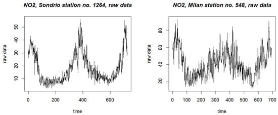
Figure 3.
AgrImOnIA data: plots of the complete series of the NO2 level, for two recording stations. The left panel is for the Sondrio station, code 1264; the right panel is for the Milan station, code 548.
In the following, we report some results obtained for the DW chart, as implemented by the Cramér–von Mises test. That chart seems to be particularly well-suited for the problem in hand because the statistical distribution of NO2 is likely to head towards a flatter, somewhat more regular behavior due to the cessation of many industrial activities during the lockdown period. Figure 4 depicts the application of the DW chart to the observations gathered by a specific recording station located in the small town of Sondrio, Lombardy. We started to control the NO2 level from the 1st of January 2020, with a burning-out set of nine previous readings. The left panel of the figure reports the first part of the series of raw data, while the right panel reports the series of the observed values of the charting statistics in (9).
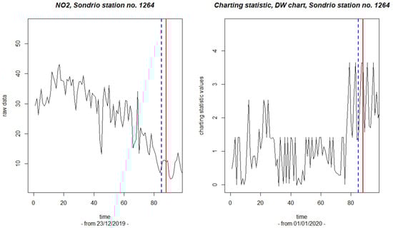
Figure 4.
Sondrio station, code 1264: plots of the NO2 raw data (left panel) and of the corresponding values of the charting statistic (right panel). The solid lines indicate the date of the first signal; the dashed lines indicate the corresponding estimate of the change point.
The threshold values were built with a 5% level of the false-alarm rate. The solid line in the right panel of Figure 4 is drawn to indicate that a threshold was overcome on the 19th of March, which is thus the date of the first signal. As known, the CP model can correspondingly provide an estimate of the change point. This estimate is the 16th of March, and it is indicated by a dashed line. Thus, the DW chart generated a prompt signal and a precise location of the lockdown for the Sondrio station, possibly with a slight delay.
Interestingly, the latter results can be compared with those obtained for a different recording station located in the center of the industrial city of Milan. As above, Figure 5 reports the first part of the raw observations (left panel) and the corresponding values computed for the charting statistic (right panel). The solid lines are drawn to indicate the date of the first signal and the dashed lines correspond to the estimated change point. One may notice that in an area where the effect of the lockdown is likely to have been stronger, the chart shows a signal earlier (27th of February) than that shown for the station in Sondrio. The estimate of the change point is also anticipated as on the 22nd of February. Thus, the results are consistent with the closure policies implemented in Lombardy and with the geo-demographic characteristics of the two specifically considered locations.
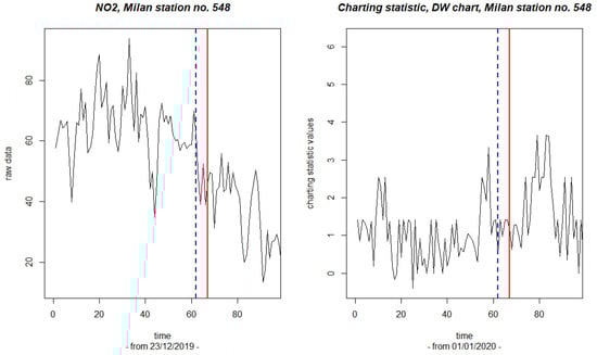
Figure 5.
Milan station, code 548: plots of the NO2 raw data (left panel) and of the corresponding values of the charting statistic (right panel). The solid lines indicate the date of the first signal; the dashed lines indicate the corresponding estimate of the change point.
As a point of comparison, we report just the final results (with no plots) obtained with the SP approach. The corresponding chart was built with the same settings as above. For the stations of Milan and Sondrio, respectively, the first signal was obtained on the 8th of October and on the 19th of January. The corresponding estimates of the change point are on the 6th of October and on the 18th of January. Thus, for the Milan station, the SP chart signaled too late, at the beginning of the second wave of the pandemic. For the Sondrio station, on the other hand, the chart provided a signal earlier than the event under study actually occurred. It should be noted that, for the same station, the following signal was on the 5th of February (estimated change point on the 4th of February); therefore, it was still too early an indication. A reasonable signal is probably the third for this chart because it occurred on the 22nd of April with an estimated change point on the 18th of March.
A remark can be added about the kind of data for which the DW chart is most suited. We cannot provide definite indications about this, except for the conclusions drawn from the simulation study reported in Section 3. In other words, we chose to apply the new method to our air quality data just because they provided the absolute certainty of the occurrence and of the positioning of some events. The application to different fields is likely to be successful as well, especially when the data have similar complexities. Specifically, the DW chart can be useful for variables that do not meet the normal assumptions and when the kind of drift to be detected goes well beyond simply location. This is markedly true for many cases in industrial quality control and in financial monitoring.
5. Conclusions and Directions for Future Research
This paper introduced a new implementation of change-point (CP) methodology and a related chart. The latter can be applied to a stream of readings without any preliminary calibration. The new implementation is made to force the comparison of just sub-samples from the stream of the same size. This has the two-fold aim to take advantage of the power of some statistical tests and to obtain symmetric sensitivity toward every directions of a possible shift. While the paper focuses on the Cramér–von Mises test, several alternative charts can be built by using any tests based on pairs of balanced samples. The choice made here aims to obtain an “omnibus” chart, that is, a tool to detect every form of change in the underlying distribution.
According to the reported simulation study, a first conclusion is that the proposed chart has indeed the “omnibus” property. Indeed, it is shown to have power not only with respect to any kind of shift from the IC distribution but also with respect to any direction. Generally speaking, this aspect is surely a positive issue, but its practical relevance highly depends on the context of application.
More specifically, one can consider the significant case of a scale shift. The DW chart shows an almost constant delay when the scale is increased or decreased by the same factor. This is definitely an uncommon feature for many control charts, which perform often very well (i.e., with a fast detection of the shift) in the case of a scale increase and, conversely, quite poorly in the opposite situation. Thus, the DW chart can be really useful when there is no prior knowledge of the direction of a scale shift. On the contrary, it is not so attractive when a scale increase is suspected or when that is the only interesting direction to be controlled.
Notice that the conclusion above holds, more broadly, for every kind of shift that can impact on the “regularity” of the IC distribution. In other words, sometimes just the shape of such a distribution may be of relevance. The DW chart can maintain similar levels of the average delay whether the shape is shifted to or from a regular, bell-like shape. Differently, other charts have an asymmetric behavior in the two cases. Thus, once again, the attractiveness of the DW chart mostly depends on the aims of the application.
Another interesting feature of the DW chart is its strong sensitivity to moderate drifts from the IC distribution. This fact shows up markedly for location, where catching small variation is, generally speaking, a rather complex task. Our simulations indicate that the DW chart responds promptly in cases where the other charts compared perform poorly. This conclusion holds when simultaneous changes in location and scale are faced as well, even if the effect of scale clearly predominates over that of location (such results are not shown in the paper, for the sake of brevity). In addition, the sensitivity of the DW chart to moderate location shifts is not affected by the shape of the underlying distribution nor by the possible presence of outliers. Such aspects need further research work, as discussed in the following.
In our opinion, the new proposal works well when applied to real data. To verify this, we analyzed some environmental data with the unusual characteristic of an (almost) known change point in a precise moment of time. Specifically, the distribution of some air quality variables showed a sudden change due to the occurrence of the lockdown period during the COVID-19 pandemic. In addition, the considered variables showed an intrinsic complexity due to many factors (measurement accuracy, seasonality, missing data, environmental issues, etc.). This perfectly justifies the use of a tool that can be powerful in the presence of any kind of drift of the IC distribution. The obtained results indicate that the DW chart provides the needed accuracy and robustness. Furthermore, our approach outperforms the classical implementation of the CP methodology, with similar settings (the SP chart). It may be underlined that, in the considered application, the underlying distribution heads toward a more regular shape as an effect of the lockdown. Thus, it is clear that such a kind of shift is an element of strength for the DW chart.
As a final point, we report here some directions for future research. We are convinced that some developments should be addressed to enable the proposed methodology to cover a wide range of applications. Some issues deserved mention already but a complete description of them is out of the scope of this introductory paper.
First, many control problems involve more than a single quality characteristic. An extension to the multivariate framework, then, is of primary importance. This problem is often made difficult due to the presence of some complex dependence structures among the observed variables. As an effect, the literature contains many tools for handling multivariate readings, often under few distributional assumptions, like data depths or spatial ranks (see the recent review by [8]). The CP methodology has been already applied by means of such tools (see [21,22]). Nonetheless, we think that, for our aims, the most promising approach comes from a preliminary dimension reduction by means of some kind of projection of the data on the real line. Such an approach is likely to provide good results even in the engaging case of high-dimensional data (as demonstrated in some recent works, like [23,24]).
A second issue to be developed concerns the reported sensitivity of the DW chart to moderate location shifts. The literature reveals that, sometimes, a joint sensitivity to moderate and large shifts may be of use. The so-called inertia problem, for instance, arises when the current observation is close to a control limit but a sudden (large) drift in the opposite direction occurs so that a fast reaction of the chart can be prevented (see [25]). Many “adaptive” schemes are proposed at achieving this aim and the most recent of which cover some peculiar aspects of quality control, such as dispersion or multivariate location. Some up-to-date contributions can be found in [26,27,28]. The connection with the DW approach is, of course, still unexplored; thus, it deserves some research work. Notice that adaptive charts often take advantage of the tools of robust statistics, a fact which can give important hints for a third development of the DW chart as a way not just to ignore but to incorporate outlying and missing observations in the monitoring process.
Author Contributions
C.G.B., M.C. and P.M.C. equally contributed to the conceptualization, development of methodology, development of software, data processing, actual writing and review. All authors have read and agreed to the published version of the manuscript.
Funding
This research received no external funding.
Data Availability Statement
The data used in this paper are openly available at https://doi.org/10.5281/zenodo.6620529, accessed on 2 September 2024 (see [20] for further details).
Conflicts of Interest
The authors declare no conflicts of interest.
Abbreviations
The following abbreviations are used in this manuscript:
| IC | in-control |
| OC | out-of-control |
| CP | change point |
| iid | independent and identically distributed |
| ARL | average run length |
| DW | dynamic window |
| SP | split |
| FW | fixed window |
| CW | constrained window |
| ME | modified EWMA |
| MC | modified CUSUM |
Appendix A. Threshold Values
Table A1.
Threshold values of the DW chart when control starts at the 10th observation. n is the current sample size and is the chosen false-alarm rate.
Table A1.
Threshold values of the DW chart when control starts at the 10th observation. n is the current sample size and is the chosen false-alarm rate.
| 10 | 2.7650 | 3.6515 | 3.6515 | 4.7673 | 4.7673 | 4.7673 |
| 11 | 2.5355 | 3.6515 | 3.6515 | 4.7673 | 4.7673 | 4.7673 |
| 12 | 2.5355 | 3.6515 | 4.1184 | 4.7673 | 5.8835 | 5.8835 |
| 13 | 2.5355 | 3.6515 | 4.1184 | 4.7673 | 5.8835 | 5.8835 |
| 14 | 2.5355 | 3.6515 | 4.4286 | 4.8571 | 5.8835 | 6.1429 |
| 15 | 2.5355 | 3.6515 | 4.1429 | 4.7673 | 5.8835 | 6.1429 |
| 16 | 2.5714 | 3.6515 | 4.5295 | 4.9029 | 5.8835 | 6.1601 |
| 17 | 2.5714 | 3.6515 | 4.5295 | 4.9029 | 5.8835 | 6.1601 |
| 18 | 2.5727 | 3.6515 | 4.7469 | 4.9643 | 5.8994 | 6.6689 |
| 19 | 2.5727 | 3.6515 | 4.7469 | 4.9643 | 5.8994 | 6.6689 |
| 20 | 2.7143 | 3.6515 | 4.7673 | 5.0730 | 6.0704 | 6.7036 |
| 21 | 2.7143 | 3.6515 | 4.7673 | 5.0730 | 6.0704 | 6.7626 |
| 22 | 2.7456 | 3.6515 | 4.7673 | 5.1817 | 6.1429 | 6.9758 |
| 23 | 2.7456 | 3.6515 | 4.7673 | 5.2129 | 6.1429 | 7.0000 |
| 24 | 2.7456 | 3.6515 | 4.7673 | 5.3394 | 6.1601 | 7.0000 |
| 25 | 2.7456 | 3.6515 | 4.7673 | 5.3825 | 6.1601 | 7.0000 |
| 26 | 2.7650 | 3.6708 | 4.7673 | 5.4286 | 6.2106 | 7.0000 |
| 27 | 2.7650 | 3.6515 | 4.7673 | 5.4286 | 6.2414 | 7.0000 |
| 28 | 2.7650 | 3.6893 | 4.7673 | 5.4326 | 6.3269 | 7.0109 |
| 29 | 2.7650 | 3.6877 | 4.7673 | 5.4326 | 6.3486 | 7.0109 |
| 30 | 2.7650 | 3.7143 | 4.7673 | 5.4719 | 6.4124 | 7.1077 |
| 35 | 2.7650 | 3.7685 | 4.7673 | 5.5574 | 6.5312 | 7.3147 |
| 40 | 2.7650 | 3.8474 | 4.7673 | 5.6678 | 6.6936 | 7.3738 |
| 45 | 2.7650 | 3.8692 | 4.7673 | 5.7252 | 6.7158 | 7.4354 |
| 50 | 2.7650 | 3.9049 | 4.7879 | 5.8097 | 6.8089 | 7.4949 |
Table A2.
Threshold values of the DW chart when control starts at the 15th observation. n is the current sample size and is the chosen false-alarm rate.
Table A2.
Threshold values of the DW chart when control starts at the 15th observation. n is the current sample size and is the chosen false-alarm rate.
| 15 | 3.6515 | 4.1184 | 4.7673 | 4.9029 | 5.8835 | 6.1429 |
| 16 | 3.6232 | 3.8772 | 4.7673 | 4.9643 | 5.8835 | 6.1601 |
| 17 | 3.1379 | 3.6515 | 4.7673 | 4.9029 | 5.8835 | 6.1601 |
| 18 | 2.9924 | 3.6515 | 4.7673 | 5.0444 | 5.8994 | 6.6689 |
| 19 | 2.8989 | 3.6515 | 4.7673 | 5.0444 | 5.8835 | 6.6689 |
| 20 | 2.8214 | 3.6515 | 4.7673 | 5.1299 | 6.0704 | 6.7036 |
| 21 | 2.7650 | 3.6515 | 4.7673 | 5.1299 | 6.1416 | 6.8316 |
| 22 | 2.7650 | 3.6515 | 4.7673 | 5.2445 | 6.1429 | 6.9758 |
| 23 | 2.7650 | 3.6515 | 4.7673 | 5.2697 | 6.1429 | 7.0000 |
| 24 | 2.7650 | 3.6573 | 4.7673 | 5.3835 | 6.1601 | 7.0000 |
| 25 | 2.7650 | 3.6515 | 4.7673 | 5.3864 | 6.1601 | 7.0000 |
| 26 | 2.7650 | 3.6764 | 4.7673 | 5.4286 | 6.2365 | 7.0000 |
| 27 | 2.7650 | 3.6598 | 4.7673 | 5.4286 | 6.2106 | 7.0000 |
| 28 | 2.7650 | 3.7143 | 4.7673 | 5.4327 | 6.3246 | 7.0109 |
| 29 | 2.7650 | 3.7143 | 4.7673 | 5.4326 | 6.3269 | 7.0109 |
| 30 | 2.7650 | 3.7299 | 4.7673 | 5.4719 | 6.3882 | 7.1033 |
| 31 | 2.7650 | 3.7264 | 4.7673 | 5.4732 | 6.4124 | 7.1033 |
| 32 | 2.7650 | 3.7619 | 4.7673 | 5.5078 | 6.4639 | 7.2126 |
| 33 | 2.7650 | 3.7619 | 4.7673 | 5.5078 | 6.4639 | 7.2457 |
| 34 | 2.7650 | 3.7685 | 4.7673 | 5.5557 | 6.5208 | 7.2755 |
| 35 | 2.7650 | 3.7685 | 4.7673 | 5.5543 | 6.5312 | 7.2789 |
| 40 | 2.7650 | 3.8480 | 4.7673 | 5.6754 | 6.6936 | 7.3558 |
| 45 | 2.7650 | 3.8772 | 4.7673 | 5.7275 | 6.7219 | 7.4383 |
| 50 | 2.7676 | 3.9163 | 4.7879 | 5.8074 | 6.8116 | 7.5004 |
Table A3.
Threshold values of the DW chart when control starts at the 20th observations. n is the current sample size and is the chosen false-alarm rate.
Table A3.
Threshold values of the DW chart when control starts at the 20th observations. n is the current sample size and is the chosen false-alarm rate.
| 20 | 3.6515 | 4.7673 | 5.1755 | 5.8835 | 6.7036 | 7.0000 |
| 21 | 3.6515 | 4.3604 | 4.8571 | 5.6585 | 6.1601 | 7.0000 |
| 22 | 3.6232 | 4.1404 | 4.7673 | 5.5078 | 6.1601 | 7.0000 |
| 23 | 3.4199 | 4.0946 | 4.7673 | 5.4286 | 6.1601 | 7.0000 |
| 24 | 3.2250 | 4.0045 | 4.7673 | 5.4719 | 6.2106 | 7.0000 |
| 25 | 3.1379 | 3.9859 | 4.7673 | 5.4286 | 6.1975 | 7.0000 |
| 26 | 2.9924 | 3.9334 | 4.7673 | 5.4719 | 6.2796 | 7.0000 |
| 27 | 2.9382 | 3.8644 | 4.7673 | 5.4403 | 6.2840 | 7.0000 |
| 28 | 2.8989 | 3.8644 | 4.7673 | 5.4972 | 6.3486 | 7.0138 |
| 29 | 2.8571 | 3.8474 | 4.7673 | 5.4824 | 6.3502 | 7.0326 |
| 30 | 2.8293 | 3.8480 | 4.7673 | 5.5078 | 6.4124 | 7.1077 |
| 35 | 2.7650 | 3.8474 | 4.7673 | 5.5574 | 6.5715 | 7.3025 |
| 40 | 2.7650 | 3.8772 | 4.7673 | 5.6759 | 6.7036 | 7.3738 |
| 41 | 2.7650 | 3.8772 | 4.7673 | 5.6912 | 6.7036 | 7.3738 |
| 42 | 2.7650 | 3.8821 | 4.7673 | 5.7252 | 6.7036 | 7.3871 |
| 43 | 2.7650 | 3.8772 | 4.7673 | 5.7252 | 6.7036 | 7.3893 |
| 44 | 2.7650 | 3.8920 | 4.7673 | 5.7370 | 6.7240 | 7.4250 |
| 45 | 2.7650 | 3.8909 | 4.7673 | 5.7370 | 6.7240 | 7.4383 |
| 46 | 2.7650 | 3.9049 | 4.7673 | 5.7666 | 6.7626 | 7.4527 |
| 47 | 2.7650 | 3.9049 | 4.7673 | 5.7684 | 6.7626 | 7.4527 |
| 48 | 2.7650 | 3.9198 | 4.7704 | 5.7817 | 6.7935 | 7.4769 |
| 49 | 2.7650 | 3.9320 | 4.7704 | 5.7966 | 6.7935 | 7.4815 |
| 50 | 2.7650 | 3.9329 | 4.7879 | 5.8139 | 6.8287 | 7.5192 |
Table A4.
Threshold values of the DW chart when control starts at the 50th observation n is the current sample size and is the chosen false-alarm rate.
Table A4.
Threshold values of the DW chart when control starts at the 50th observation n is the current sample size and is the chosen false-alarm rate.
| 50 | 4.7673 | 5.7931 | 6.4735 | 7.2318 | 8.1674 | 8.9235 |
| 51 | 4.1082 | 5.0699 | 5.8835 | 6.6742 | 7.6253 | 8.3517 |
| 52 | 3.7143 | 4.8158 | 5.7075 | 6.3701 | 7.3709 | 8.1279 |
| 53 | 3.6515 | 4.7673 | 5.4824 | 6.1656 | 7.2463 | 8.0566 |
| 54 | 3.6515 | 4.7673 | 5.3991 | 6.1429 | 7.1510 | 7.9540 |
| 55 | 3.6515 | 4.7579 | 5.2957 | 6.0860 | 7.0648 | 7.9358 |
| 56 | 3.6515 | 4.5873 | 5.2044 | 6.0304 | 7.0138 | 7.9106 |
| 57 | 3.6515 | 4.4904 | 5.1299 | 5.9591 | 7.0000 | 7.8618 |
| 58 | 3.6244 | 4.4254 | 5.0837 | 5.9200 | 7.0000 | 7.8652 |
| 59 | 3.5301 | 4.3598 | 5.0488 | 5.8876 | 7.0000 | 7.8288 |
| 60 | 3.4503 | 4.2840 | 5.0219 | 5.8835 | 7.0000 | 7.8288 |
| 61 | 3.3931 | 4.2199 | 4.9710 | 5.8835 | 7.0000 | 7.8207 |
| 62 | 3.2857 | 4.1894 | 4.9623 | 5.8835 | 7.0000 | 7.8184 |
| 63 | 3.2225 | 4.1429 | 4.9345 | 5.8835 | 7.0000 | 7.7965 |
| 64 | 3.1554 | 4.1429 | 4.9103 | 5.8835 | 7.0000 | 7.8059 |
| 65 | 3.1379 | 4.1429 | 4.9029 | 5.8835 | 7.0000 | 7.7841 |
| 70 | 2.9924 | 4.1184 | 4.9029 | 5.8835 | 7.0000 | 7.8059 |
| 75 | 2.9417 | 4.1184 | 4.9029 | 5.8835 | 7.0000 | 7.8066 |
| 80 | 2.9417 | 4.1184 | 4.9029 | 5.8835 | 7.0000 | 7.8375 |
| 85 | 2.9069 | 4.1184 | 4.9029 | 5.8835 | 7.0000 | 7.8629 |
| 90 | 2.8983 | 4.1184 | 4.9029 | 5.8835 | 7.0000 | 7.8856 |
| 95 | 2.8785 | 4.1184 | 4.9029 | 5.8835 | 7.0000 | 7.9097 |
| 100 | 2.8571 | 4.1184 | 4.9029 | 5.8835 | 7.0000 | 7.9358 |
Table A5.
Threshold values of the DW chart when control starts at the 100th observation. n is the current sample size and is the chosen false-alarm rate.
Table A5.
Threshold values of the DW chart when control starts at the 100th observation. n is the current sample size and is the chosen false-alarm rate.
| 100 | 5.2697 | 6.3642 | 7.1950 | 8.0274 | 9.0900 | 9.8778 |
| 101 | 4.5812 | 5.6619 | 6.4525 | 7.2976 | 8.3637 | 9.1936 |
| 102 | 4.1466 | 5.2931 | 6.1295 | 7.0000 | 8.0733 | 8.8622 |
| 103 | 3.9176 | 5.0367 | 5.8835 | 6.7898 | 7.8564 | 8.6604 |
| 104 | 3.7143 | 4.9029 | 5.8384 | 6.6486 | 7.7136 | 8.5368 |
| 105 | 3.6515 | 4.7886 | 5.7119 | 6.5112 | 7.5946 | 8.4353 |
| 106 | 3.6515 | 4.7673 | 5.6047 | 6.4124 | 7.5070 | 8.3536 |
| 107 | 3.6515 | 4.7673 | 5.5172 | 6.3382 | 7.4383 | 8.2882 |
| 108 | 3.6515 | 4.7085 | 5.4558 | 6.2786 | 7.3973 | 8.2469 |
| 109 | 3.6515 | 4.6409 | 5.4286 | 6.2115 | 7.3558 | 8.1950 |
| 110 | 3.6515 | 4.5873 | 5.3871 | 6.1656 | 7.3558 | 8.1608 |
| 111 | 3.6515 | 4.5295 | 5.3334 | 6.1498 | 7.3468 | 8.1428 |
| 112 | 3.6515 | 4.4853 | 5.2917 | 6.1429 | 7.3147 | 8.1223 |
| 113 | 3.6515 | 4.4286 | 5.2445 | 6.1429 | 7.2921 | 8.1168 |
| 114 | 3.5637 | 4.4167 | 5.2091 | 6.1339 | 7.2540 | 8.1168 |
| 115 | 3.5193 | 4.3718 | 5.1755 | 6.1022 | 7.2457 | 8.1168 |
| 116 | 3.5132 | 4.3450 | 5.1481 | 6.0712 | 7.2270 | 8.1168 |
| 117 | 3.4503 | 4.3088 | 5.1201 | 6.0523 | 7.2066 | 8.1168 |
| 118 | 3.3193 | 4.2502 | 5.0991 | 6.0397 | 7.1846 | 8.1168 |
| 119 | 3.2739 | 4.2502 | 5.0730 | 6.0090 | 7.1736 | 8.1168 |
| 120 | 3.2857 | 4.2298 | 5.0730 | 6.0024 | 7.1686 | 8.1168 |
| 125 | 3.1312 | 4.1429 | 5.0015 | 5.9261 | 7.1079 | 8.1168 |
| 130 | 3.0225 | 4.1429 | 4.9436 | 5.8994 | 7.0865 | 8.1168 |
| 140 | 2.9417 | 4.1184 | 4.9036 | 5.8835 | 7.0666 | 8.0753 |
| 150 | 2.9417 | 4.1184 | 4.9029 | 5.8835 | 7.0458 | 8.0493 |
References
- Montgomery, D.C. Introduction to Statistical Quality Control; John Wiley & Sons: Hoboken, NJ, USA, 2013. [Google Scholar]
- Qiu, P. Introduction to Statistical Process Control; CRC Press: Boca Raton, FL, USA, 2014. [Google Scholar]
- Hou, S.; Yu, K. A non-parametric CUSUM control chart for process distribution change detection and change type diagnosis. Int. J. Prod. Res. 2021, 59, 1166–1186. [Google Scholar] [CrossRef]
- Talordphop, K.; Areepong, Y.; Sukparungsee, S. Design and Analysis of Extended Exponentially Weighted Moving Average Signed-Rank Control Charts for Monitoring the Process Mean. Mathematics 2023, 11, 4482. [Google Scholar] [CrossRef]
- Weiß, C.H.; Testik, M.C. Nonparametric control charts for monitoring serial dependence based on ordinal patterns. Technometrics 2023, 65, 340–350. [Google Scholar] [CrossRef]
- Ali, S.; Abbas, Z.; Nazir, H.Z.; Riaz, M.; Zhang, X.; Li, Y. On designing non-parametric EWMA sign chart under ranked set sampling scheme with application to industrial process. Mathematics 2020, 8, 1497. [Google Scholar] [CrossRef]
- Xie, X.; Qiu, P. Control charts for dynamic process monitoring with an application to air pollution surveillance. Ann. Appl. Stat. 2023, 17, 47–66. [Google Scholar] [CrossRef]
- Qiu, P. Some perspectives on nonparametric statistical process control. J. Qual. Technol. 2018, 50, 49–65. [Google Scholar] [CrossRef]
- Chakraborti, S.; Graham, M. Nonparametric Statistical Process Control; John Wiley and Sons Inc.: New York, NY, USA, 2019. [Google Scholar]
- Chakraborti, S.; Van Der Laan, P.; Bakir, S.T. Nonparametric Control Charts: An Overview and Some Results. J. Qual. Technol. 2001, 33, 304–315. [Google Scholar] [CrossRef]
- Hawkins, D.M.; Qiu, P.; Kang, C.W. The changepoint model for statistical process control. J. Qual. Technol. 2003, 35, 355–366. [Google Scholar] [CrossRef]
- Capizzi, G. Recent advances in process monitoring: Nonparametric and variable-selection methods for phase I and phase II. Qual. Eng. 2015, 27, 44–67. [Google Scholar] [CrossRef]
- Hawkins, D.M.; Deng, Q. A nonparametric change-point control chart. J. Qual. Technol. 2010, 42, 165–173. [Google Scholar] [CrossRef]
- Hawkins, D.M.; Zamba, G.K.D. Statistical process control for shifts in mean or variance using a changepoint formulation. Technometrics 2005, 47, 164–173. [Google Scholar] [CrossRef]
- Ross, G.J.; Tasoulis, D.K.; Adams, N.M. Nonparametric monitoring of data streams for changes in location and scale. Technometrics 2011, 53, 379–389. [Google Scholar] [CrossRef]
- Ross, G.J.; Adams, N.M. Two nonparametric control charts for detecting arbitrary distribution changes. J. Qual. Technol. 2012, 44, 102–116. [Google Scholar] [CrossRef]
- Anderson, T.W. On the Distribution of the Two-Sample Cramer–Von Mises Criterion. Ann. Math. Stat. 1962, 33, 1148–1159. [Google Scholar] [CrossRef]
- Zou, C.; Tsung, F. Likelihood ratio-based distribution-free EWMA control charts. J. Qual. Technol. 2010, 42, 174–196. [Google Scholar] [CrossRef]
- Zhang, J. Powerful goodness-of-fit tests based on the likelihood ratio. J. R. Stat. Soc. Ser. B Stat. Methodol. 2002, 64, 281–294. [Google Scholar] [CrossRef]
- Fassò, A.; Rodeschini, J.; Fusta Moro, A.; Shaboviq, Q.; Maranzano, P.; Cameletti, M.; Finazzi, F.; Golini, N.; Ignaccolo, R.; Otto, P. Agrimonia: A dataset on livestock, meteorology and air quality in the Lombardy region, Italy. Sci. Data 2023, 10, 143. [Google Scholar] [CrossRef] [PubMed]
- Holland, M.D.; Hawkins, D.M. A Control Chart Based on A Nonparametric Multivariate Change-Point Model. J. Qual. Technol. 2014, 46, 63–77. [Google Scholar] [CrossRef]
- Kim, J.M.; Wang, N.; Liu, Y. Multi-stage change point detection with copula conditional distribution with PCA and functional PCA. Mathematics 2020, 8, 1777. [Google Scholar] [CrossRef]
- Chakraborty, N.; Lui, C.F.; Maged, A. A distribution-free change-point monitoring scheme in high-dimensional settings with application to industrial image surveillance. Commun. Stat.-Simul. Comput. 2023, 53, 5858–5874. [Google Scholar] [CrossRef]
- Mukherjee, A.; Marozzi, M. Nonparametric Phase-II control charts for monitoring high-dimensional processes with unknown parameters. J. Qual. Technol. 2022, 54, 44–64. [Google Scholar] [CrossRef]
- Capizzi, G.; Masarotto, G. An Adaptive Exponentially Weighted Moving Average Control Chart. Technometrics 2003, 45, 199–207. [Google Scholar] [CrossRef]
- Zaman, B.; Mahfooz, S.; Mehmood, R.; Khan, N.; Imran, T. An adaptive EWMA control chart based on Hampel function to monitor the process location parameter. Qual. Reliab. Eng. Int. 2023, 39, 1277–1298. [Google Scholar] [CrossRef]
- Arshad, A.; Noor-ul Amin, M.; Hanif, M. Monitoring of coefficient of variation with function-based adaptive exponentially weighted moving average control chart. Qual. Reliab. Eng. Int. 2022, 38, 1074–1091. [Google Scholar] [CrossRef]
- Riaz, M.; Zaman, B.; Raji, I.; Omar, M.; Mehmood, R.; Abbas, N. An Adaptive EWMA Control Chart Based on Principal Component Method to Monitor Process Mean Vector. Mathematics 2022, 10, 2025. [Google Scholar] [CrossRef]
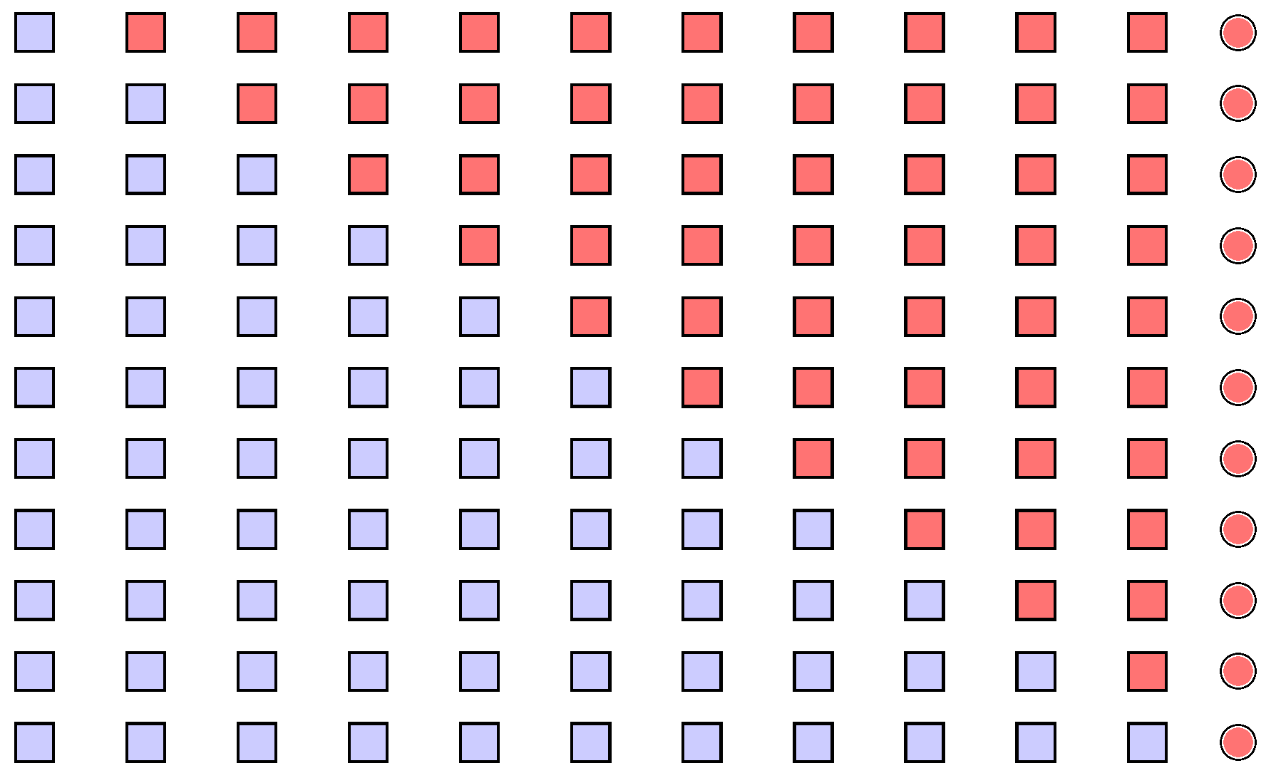
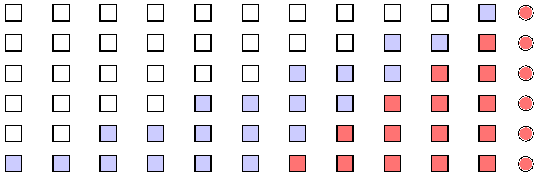
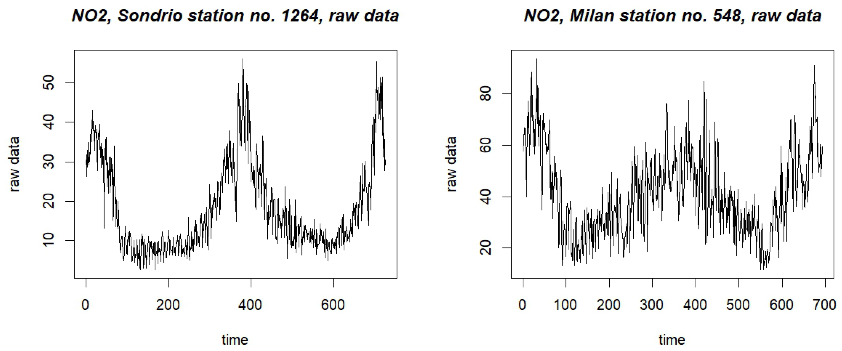
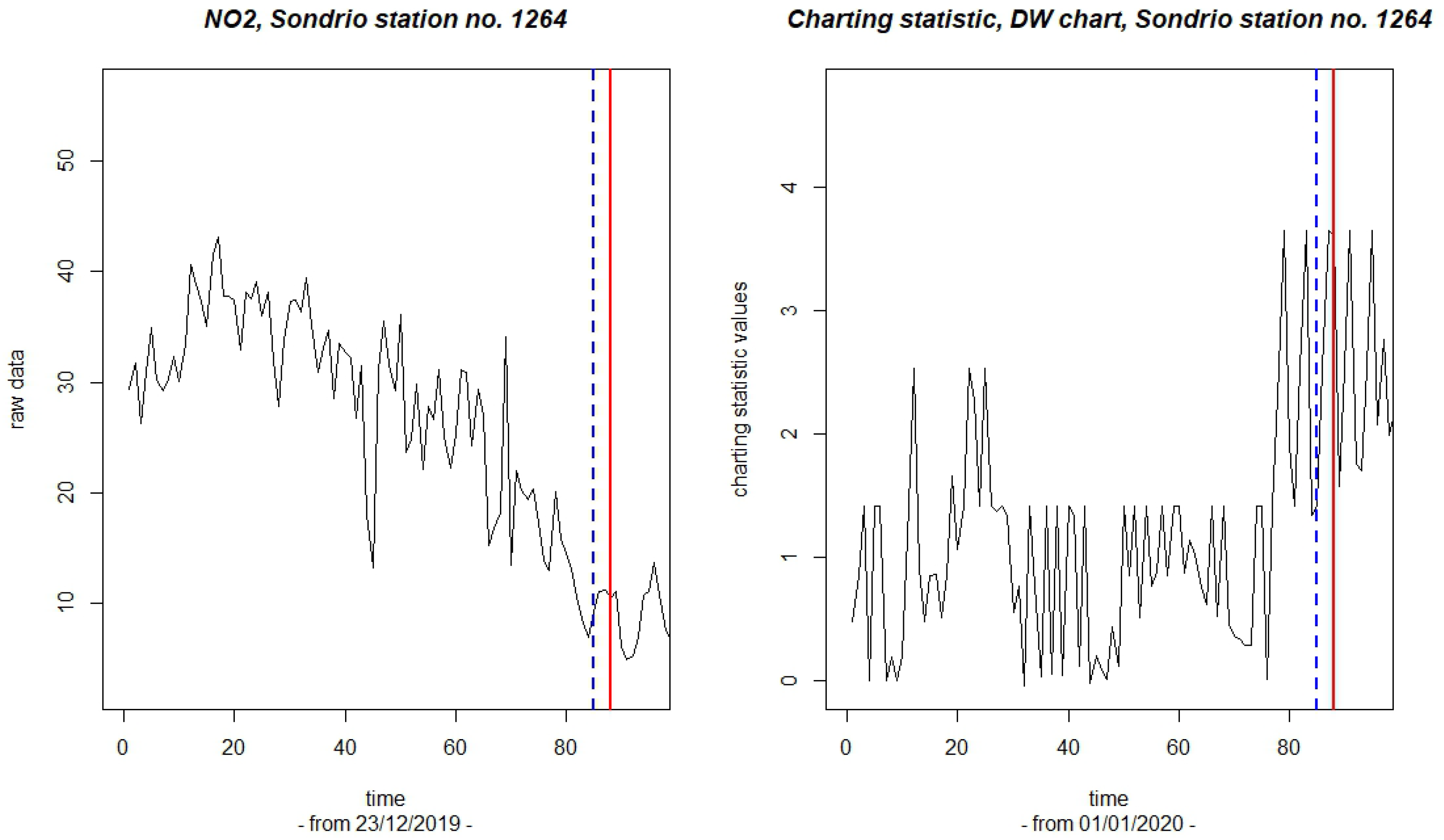
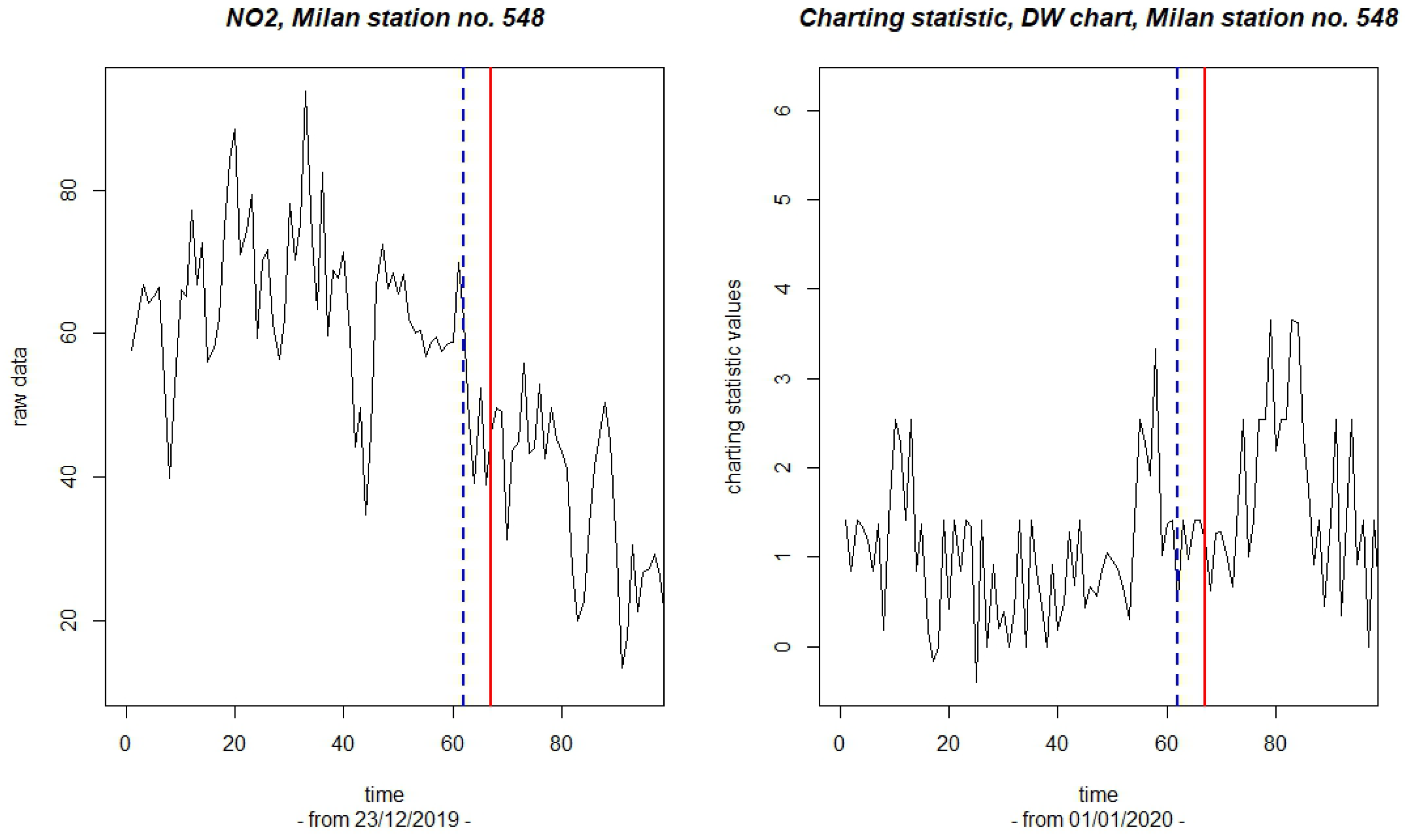
Disclaimer/Publisher’s Note: The statements, opinions and data contained in all publications are solely those of the individual author(s) and contributor(s) and not of MDPI and/or the editor(s). MDPI and/or the editor(s) disclaim responsibility for any injury to people or property resulting from any ideas, methods, instructions or products referred to in the content. |
© 2025 by the authors. Licensee MDPI, Basel, Switzerland. This article is an open access article distributed under the terms and conditions of the Creative Commons Attribution (CC BY) license (https://creativecommons.org/licenses/by/4.0/).