Vibration of the Liénard Oscillator with Quadratic Damping and Constant Excitation

Abstract

In this paper, the Liénard oscillator with nonlinear deflection, quadratic damping, and constant excitation is considered. In general, there is no analytic solution for the Liénard equation. However, for certain parameter values, the exact analytic solution exists and has the form of the Ateb function. In addition, for the oscillator with weakly perturbed parameters, the approximate analytic solution is obtained. For the considered Liénard equation, independently of parameter values, the first integral is found. The main advantage of the first integral is that after simple analysis and without solving the equation of motion, it gives important data about oscillation: the dependence of vibration on initial conditions and on the variation of the constant of excitation. In addition, by integration of the first integral, the period of vibration follows. The results of the research on the Liénard equation are applied for optimization of the properties of a sieve in the process industry. For the sieve with mass variation, dependent on the displacement function, the influence of excitation force on the system vibration is analyzed, and the optimal value is suggested.

1. Introduction

Back in 1928, the French physicist and engineer Alfred-Marie Liénard, who was dealing with the problems of elasticity, magnetism, and mechanics, introduced the following second-order differential equation [1]:

$$\ddot{x}+f\left(x\right)\dot{x}+g\left(x\right)=0,$$

(1)

where $f\left(x\right)$ and $g\left(x\right)$ are linear or nonlinear functions dependent on x. Since that time, the equation has been extended, adopted, and modified with the aim to describe phenomena in mechanics, engineering, economics, biological sciences, physics, and other scientific fields. Thus, in 1942, Equation (1) was extended as follows [2]:

$$\ddot{x}+f\left(x,\dot{x}\right)\dot{x}+g\left(x\right)=0,$$

(2)

where $f$ is not only the function of $x$ but also of $\dot{x}$. This model corresponds to the relaxation oscillator. The elastic term $g\left(x\right)$ is assumed to be a linear, quadratic, or cubic function of $x$. At the other side, the Liénard equation is modified by introducing relativistic acceleration [3,4], as follows:

$${\displaystyle \frac{d}{dt}}\left({\displaystyle \frac{\dot{x}{\left|\dot{x}\right|}^{p-2}}{{(1-{\left|\dot{x}\right|}^p)}^{\frac{p-1}{p}}}}\right)+f\left(x\right)\dot{x}+g\left(x\right)=0,$$

(3)

where $p\ge 2$. However, the most often applied Liénard equation has the form

$$f_1\left(x\right)\ddot{x}+cx+b\dot{x}+f_2\left(x\right)\dot{x}+g^{*}\left(x\right)x=0,$$

(4)

where $f_1\left(x\right)$, $f_2\left(x\right)$, and $g^{*}\left(x\right)$ are polynomial functions, and c and b are constants. The model (2) is characterized by multiple constitutive relations rather than a single one, leading to its extensive utilization in various fields of engineering and science. Let us mention some of them.

The fast development of nanotechnology and material science has led to skyrocketing interest in micro-electromechanical systems (MEMS). In [5,6] the oscillation of the MEMS is investigated by analyzing the solution of Equation (2). Equation (2) gives the free vibration of the magneto-electro-mechanical oscillator with a magnet–coil system [7,8] where the interaction between a pair of neodymium permanent magnets is replaced with a nonlinear instead of linear stiffness relation. The model gives the explanation about the frequency and amplitude properties of the system. The same model of magnetic interaction is applied in free vibrations of the horizontal mathematical pendulum in a repulsive field controlled by two coil magnets [9]. Using the appropriate parameter values, the analytic model gives good simulation of the experimentally obtained results. Equation (2) is utilized for the effect of spontaneous emission and gain saturation in directly modulated semiconductor lasers [10], too. The model is suitable for qualitative analysis of the problem. Equation (2), with certain parameter values, is applied in treating heat conduction, too. Namely, the mathematical model of one-directional heat conduction, given with the Maxwell–Cattaneo equation (which is a special case of the telegraph equation), is transformed into the averaged time Equation (2) [11]. The solution of the equation gives the heat distribution in time. The nonlinear model is strong and gives better results than the linear one.

Due to analogies in science, Equation (2) is applied in treating phenomena in biology, human sciences, etc. Let us mention some of them. The bacteria growing in a chemostat depending on the nutrient levels is modeled with Equation (2) (see [12]). The solution of the equation gives the influence of the variation of the chemostat concentration on the bacteria density. The spread of a disease within a given population [13] is a seemingly necessary condition of human existence, leading to the presence of epidemics. In the papers [14,15,16], the epidemiological model based on the Michaelis–Menten contact rate is given in the form (2). By analyzing the model, the effect of two subpopulations—susceptibles (those who can catch or acquire the disease but presently do not have it) and infectives (those who have the disease and can transmit it to the susceptibles)—is obtained.

Based on the aforementioned research, it can be concluded that the common property of processes and motions is their periodicity. Hence, the Liénard equation has to satisfy the conditions for existence of the unique periodic solution (see [17,18]). In addition, it is concluded that up to nowadays, a significant number of approximate procedures have been developed for solving the nonlinear Liénard equation (see, for example, [19]). Most of them are based on the exact solution of the linearized equation. Unfortunately, the obtained results are not accurate enough, and the so-obtained analytic solutions differ significantly in comparison to the exact numeric ones. The discrepancy is due to the fact that in solving the procedure, the strong nonlinear terms are transformed into weak nonlinear or simple linear ones. However, the Liénard equation is strong and nonlinear and in general contains the nonlinear deflection and damping term.

In this paper, the following special type of Liénard equation is considered:

$$\left(1+x\right)\ddot{x}+f_2\left({\dot{x}}^2\right)+g^{*}\left(x\right)=\mathcal{F},$$

(5)

where the deflection function $g^{*}\left(x\right)$ is of power type, $f_2\left({\dot{x}}^2\right)$ is the function dependent on quadratic damping, and $\mathcal{F}$ is a constant value. By investigating the Liénard oscillator (5) with nonlinear deflection and quadratic damping, deeper insights into the interplay between nonlinearity, dissipation, and complex dynamics can be recovered. The equation is an appropriate model for the damped mass-variable oscillatory system with one degree of freedom and excited with a constant force. Unlike the previously mentioned methods, in this paper, a procedure for solving Equation (5) based on the exact solution of a strictly nonlinear differential equation is developed. However, obtaining closed-form solutions for the nonlinear Equation (5) is often challenging. In this paper, the exact solution is obtained by modifying the harmonic balance method and utilizing the cosine Ateb function [20]. Based on that closed-form solution, the analytic solution of Equation (5) is determined by adopting the approximate averaging solving method published in [21,22]. The obtained analytic result is tested on an example, the approximate solution is compared with a numeric one, and the difference is determined. In this paper, the first integral for the Liénard equation is composed. The integral is analyzed for various values of system parameters and excitation constant. By integrating the first integral, the period of vibration of the oscillator is computed. Finally, the results of this study on the Liénard equation are applied for optimizing the excitation parameter of the sieve, which is modeled as a mass-variable oscillator.

This paper has six sections. In Section 2, the procedure for solving the Liénard equation is presented in general. In Section 3, the exact analytic solution for the equation with certain parameters is obtained. In this study, it is shown that despite strong nonlinearity and quadratic damping, such an oscillator may have simple harmonic motion. The approximate solution based on the exact one is determined for the perturbed equation. In Section 4, the first integral of the Liénard equation is introduced. Using the first integral, the influence of initial conditions and variation of the excitation is analyzed. By integrating, a formula for period of vibration is obtained. In Section 5, as a numerical example, the vibration of a sieve with variable mass for some values of excitation is considered. The paper ends with the Conclusions Section.

2. Exact and Approximate Solution of the Generalized Liénard Equation

To obtain the exact solution of the generalized Liénard equation of the type (5), the following procedure is developed:

-

For Equation (5), the trial solution is assumed in the form of a periodic function x(t) = x(t + T) with period T.

-

Substituting the trial solution into (5) and using the harmonic balance method by equating the terms with the same order of the assumed function, a system of algebraic equations is obtained.

-

By solving algebraic equations, the coefficients in Equation (5) and the parameters of the solution are obtained. The so-obtained solution is the closed form one for the equation

$$\left(1+x\right)\ddot{x}+{\overline{f}}_2\left({\dot{x}}^2\right)+{\overline{g}}^{*}\left(x\right)=0,$$

(6)

where ${\overline{f}}_2\left(x\right)$ and ${\overline{g}}^{*}\left(x\right)$ are the functions with corresponding coefficients.

Comparing (5) and (6), it is evident that there is a difference. Let us assume that the difference is small, and (5) is the perturbed version of (6). Then, the solution of (5) has to be also the perturbed version of the closed-form solution of (6).

Hence, Equation (5) is transformed into

$$\left(1+x\right)\ddot{x}+{\overline{f}}_2\left({\dot{x}}^2\right)+{\overline{g}}^{*}\left(x\right)=({\overline{f}}_2\left({\dot{x}}^2\right)-f_2\left({\dot{x}}^2\right)+\left({\overline{g}}^{*}\left(x\right)-g^{*}\left(x\right)\right).$$

(7)

Introducing the solution for (7) in the form of the solution for (6), but with time-variable amplitude and phase, Equation (7) is transformed into two first-order differential equations in the two new variables: amplitude and phase.

To find the exact solution for the aforementioned system is a hard task. For simplicity, the averaging procedure over the period of the periodic functions is performed, and the averaged equations follow.

The solutions of these equations give the averaged solution of (5).

Remark 1.

The difference between Equations (5) and (6) may be in the parameter values but also in terms, i.e., in the structure of the equation.

3. Liénard Oscillator with a Constant Excitation

For the case when $f_2\left({\dot{x}}^2\right)=$ ${\displaystyle \frac{1}{2}}{\dot{x}}^2$ and $g^{*}\left(x\right)=x{\left|x\right|}^{\alpha -1}\left(1+c_{\alpha }x\right),$ Equation (5) is

$$\ddot{x}\left(1+x\right)+x{\left|x\right|}^{\alpha -1}\left(1+c_{\alpha }x\right)+{\displaystyle \frac{1}{2}}{\dot{x}}^2-\mathcal{F}=0,$$

(8)

where $\mathcal{F}$ and $c_{\mathrm{\alpha }}$ are constants, and $\alpha \ge 0$ is any integer or non-integer. The equation is a power-type nonlinear equation with quadratic damping and the constant excitation $\mathcal{F}$. In this paper, the periodic solution of Equation (8) for the initial conditions

$$x\left(0\right)=x_0<\left|1\right|, \dot{x}\left(0\right)={\dot{x}}_0<\left|1\right|$$

is considered. Namely, analyzing Equation (8), it is evident that (8) has the singularity for $x=-1.$

3.1. Exact Solution

The solution is assumed in the form of the periodic function [20]

$$x=A\mathrm{ca}\left(\alpha ,1, \omega t+\theta \right)$$

(9)

where $\mathrm{ca}\left(\alpha ,1, \omega t+\theta \right)$ is the cosine Ateb function, and $A$, $\theta$, and $\omega$ are the amplitude, initial phase, and frequency. The cosine Ateb function is defined as the inverse version of the incomplete beta function [23]. The first and the second time derivatives of (9) are

$$\dot{x}=-A\omega {\displaystyle \frac{2}{\alpha +1}}\mathrm{sa}\left(1,\alpha , \omega t+\theta \right),\ddot{x}=-A{\omega }^2{\displaystyle \frac{2}{\alpha +1}}{\mathrm{ca}}^{\alpha }\left(\alpha ,1, \omega t+\theta \right),$$

(10)

where $\mathrm{sa}\left(1,\alpha , \omega t+\theta \right)$ is the sine Ateb function [24].

Remark 2.

For simplicity, instead of $\mathrm{ca}\left(\alpha ,1, \omega t+\theta \right)$ and $\mathrm{sa}\left(1,\alpha , \omega t+\theta \right)$, the notations $\mathrm{ca}$ and $\mathrm{sa}$ will be used, respectively.

Substituting (9) and (10) into (8), using the relation [24]

$${\mathrm{sa}}^2+{\mathrm{ca}}^{\alpha +1}=1,$$

(11)

and after separation of terms with the same order of ca function, the following system of linear equations is obtained:

$${\mathrm{ca}}^{\alpha +1}: c_{\alpha }={\displaystyle \frac{\alpha +2}{\alpha +1}},{\mathrm{ca}}^{\alpha }: {\omega }^2={\displaystyle \frac{\alpha +1}{2}}{A}^{\alpha -1}, {\mathrm{ca}}^0: \mathcal{F}={\displaystyle \frac{A^{\alpha +1}}{\alpha +1}}$$

(12)

Finally, it follows that for ${\mathcal{F}}^{*}={\displaystyle \frac{A^{\alpha +1}}{\alpha +1}}$ and $c_{\alpha }^{*}={\displaystyle \frac{\alpha +2}{\alpha +1}}$ the equation

$$\ddot{x}\left(1+x\right)+x{\left|x\right|}^{\alpha -1}\left(1+c_{\alpha }^{*}x\right)+{\displaystyle \frac{1}{2}}{\dot{x}}^2-{\mathcal{F}}^{*}=0,$$

(13)

has the exact solution

$$x=A\mathrm{ca}\left(\alpha ,1,\sqrt{{\displaystyle \frac{\alpha +1}{2}}{A}^{\alpha -1}} t+\theta \right),$$

(14)

where $A$ and $\theta$ are arbitrary constants that depend on the initial conditions. In spite of the fact that the oscillator has quadratic damping, the frequency and the amplitude of vibration are constant for certain parameter values.

Remark 3.

The solution (14) is the closed form one for the Liénard Equation (13) with certain values of ${\mathcal{F}}^{*}$ and $c_{\alpha }^{*}$. Unfortunately, it is not the analytic solution of Equation (8) in general.

3.2. Approximate Solution for the Oscillator with Small Perturbation

For the case when the parameters of the terms in (8) differ from those given in the ‘exact’ Equation (13), according to (7), we have

$$\ddot{x}\left(1+x\right)+x{\left|x\right|}^{\alpha -1}\left(1+c_{\alpha }^{*}x\right)+{\displaystyle \frac{1}{2}}{\dot{x}}^2-{\mathcal{F}}^{*}=\epsilon \mathrm{\Phi }\left(x,\dot{x}\right),$$

(15)

where $\epsilon \mathrm{\Phi }\left(x,\dot{x}\right)$ is the function that gives the difference between the exact Equation (13) and general Equation (8), and $\mathrm{\epsilon }<1$ is a small parameter.

For the small function $\epsilon \mathrm{\Phi }\left(x,\dot{x}\right)$ with parameter $\mathrm{\epsilon }\ll 1$, the approximate solution of Equation (15) is assumed as the perturbed version of the exact solution (9) with time variable amplitude $A\left(t\right)$ and phase $\psi \left(t\right)$:

$$x=A\left(t\right)\mathrm{ca}\left(\alpha ,1,\psi \left(t\right)\right).$$

(16)

For

$$\dot{\psi }\left(t\right)=\omega \left(t\right)+\dot{\theta }\left(t\right),$$

(17)

$\theta \left(t\right)$ is the time-variable function, and

$$\omega \left(t\right)=\sqrt{{\displaystyle \frac{\alpha +1}{2}}A{\left(t\right)}^{\alpha -1}},$$

(18)

is the time-variable frequency of the Ateb function. Assuming $\dot{x}$ in the form (10), i.e.,

$$\dot{x}=-A\left(t\right)\omega \left(t\right){\displaystyle \frac{2}{\alpha +1}}\mathrm{sa}\left(1,\alpha ,\psi \left(t\right)\right),$$

(19)

and comparing it with the first time derivative of (16), the constraint yields

$$\dot{A}\left(t\right)\mathrm{ca}-A\left(t\right)\dot{\theta }\left(t\right){\displaystyle \frac{2}{\alpha +1}}\mathrm{sa}=0.$$

(20)

Substituting (16)–(19) and the time derivative of (19) into (15), it is

$$-\dot{A}\left(t\right)\omega \left(t\right)\mathrm{sa}-A\left(t\right)\omega \left(t\right)\dot{\theta }\left(t\right){\displaystyle \frac{2}{\alpha +1}}{\mathrm{ca}}^{\alpha }=\epsilon \mathrm{\Phi }\left(A\left(t\right)\mathrm{ca},-A\left(t\right)\omega \left(t\right){\displaystyle \frac{2}{\alpha +1}}\mathrm{sa}\right).$$

(21)

Equations (20) and (21) are the coupled first-order equations that correspond to (15). After some modification, it yields

$$\dot{A}\left(t\right)\omega \left(t\right)=-\epsilon \mathrm{\Phi }\left(A\left(t\right)\mathrm{ca},-A\left(t\right)\omega \left(t\right){\displaystyle \frac{2}{\alpha +1}}\mathrm{sa}\right)\mathrm{sa},$$

(22)

$$A\left(t\right)\omega \left(t\right)\dot{\theta }\left(t\right){\displaystyle \frac{2}{\alpha +1}}=-\epsilon \mathrm{\Phi }\left(A\left(t\right)\mathrm{ca},-A\left(t\right)\omega \left(t\right){\displaystyle \frac{2}{\alpha +1}}\mathrm{sa}\right)\mathrm{ca}.$$

(23)

After averaging the sa and ca function over the period $T$ of Ateb function $T=2B\left({\displaystyle \frac{1}{\alpha +1}},{\displaystyle \frac{1}{2}}\right)$, where $B$ is the complete beta function [20], the averaged equations follow as

$$\dot{A}\left(t\right)\omega \left(t\right)=-\epsilon \mathrm{\Phi }\left(A\left(t\right)\mathrm{ca},-A\left(t\right)\omega \left(t\right){\displaystyle \frac{2}{\alpha +1}}\mathrm{sa}\right)\mathrm{sa},$$

(24)

$$A\left(t\right)\omega \left(t\right)\dot{\theta }\left(t\right){\displaystyle \frac{2}{\alpha +1}}=-\epsilon \mathrm{\Phi }\left(A\left(t\right)\mathrm{ca},-A\left(t\right)\omega \left(t\right){\displaystyle \frac{2}{\alpha +1}}\mathrm{sa}\right)\mathrm{ca},$$

(25)

where $\langle ·\rangle ={\displaystyle \frac{1}{T}}\underset{0}{\overset{T}{{\displaystyle \int }}}\left(·\right)dt$.

Solving (24) and (25), the approximate amplitude and phase functions are obtained.

3.3. Example

Let us consider the equation

$$\ddot{x}\left(1+x\right)+x{\left|x\right|}^{\alpha -1}\left(1.1+c_{\alpha }^{*}x\right)+{\displaystyle \frac{1}{2}}{\dot{x}}^2-{\mathcal{F}}^{*}=0.$$

(26)

According to (7), Equation (26) is rewritten in the form

$$\ddot{x}\left(1+x\right)+x{\left|x\right|}^{\alpha -1}\left(1+c_{\alpha }^{*}x\right)+{\displaystyle \frac{1}{2}}{\dot{x}}^2-{\mathcal{F}}^{*}=-\epsilon x{\left|x\right|}^{\alpha -1},$$

(27)

where the left side of (27) is the exact Equation (13), and $\epsilon =0.1$. Using (24) and (25), the relation (27) is transformed into two averaged first-order differential equations:

$$\dot{A}\left(t\right)\omega \left(t\right)=\epsilon A^{\alpha }{\mathrm{ca}}^{\alpha }\mathrm{sa},A\left(t\right)\omega \left(t\right)\dot{\theta }\left(t\right){\displaystyle \frac{2}{\alpha +1}}=\epsilon A^{\alpha }{\mathrm{ca}}^{\alpha +1}.$$

(28)

Using the expression (18), the relation (11) and the averaged values of Ateb functions [20], ${\mathrm{ca}}^{\mathrm{\alpha }}\mathrm{sa}=0$ and ${\mathrm{sa}}^2={\displaystyle \frac{\alpha +1}{\alpha +3}}$, Equation (28) yields

$$\dot{A}\left(t\right)=0,\dot{\theta }\left(t\right)=\epsilon A{\left(t\right)}^{\left(\alpha -1\right)/2}{\displaystyle \frac{2}{\alpha +3}}\sqrt{{\displaystyle \frac{\alpha +1}{2}}}.$$

(29)

After integration, A = const, $\theta =\epsilon A^{\left(\alpha -1\right)/2}t{\displaystyle \frac{2}{\alpha +3}}\sqrt{{\displaystyle \frac{\alpha +1}{2}}}$, and the averaged solution is

$$x=A\mathrm{ca}\left(\alpha ,1,A^{{\displaystyle \frac{\alpha -1}{2}}}t\sqrt{{\displaystyle \frac{\alpha +1}{2}}}\left(1+{\displaystyle \frac{2\epsilon }{\alpha +3}}\right)\right),$$

(30)

where

$${\omega }_a=A^{{\displaystyle \frac{\alpha -1}{2}}}\sqrt{{\displaystyle \frac{\alpha +1}{2}}}\left(1+{\displaystyle \frac{2\epsilon }{\alpha +3}}\right).$$

(31)

Comparing the exact solution (14) for (13) and the approximate solution (30) for (26), it is evident that there is a difference between the exact frequency (18) and the approximate one (31).

In

Table 1. The frequency rate ω_a/ω as the function of the order of nonlinearity α.

α	1	1.5	2	3	5
ωa/ω	1.050	1.044	1.040	1.033	1.025

, the frequency rate of the exact frequency (18) and of the approximate one (31) for ε = 0.1 and various orders of nonlinearity $\alpha$ are shown.

It is obtained that the frequency of the perturbed equation is higher than of the exact one. The frequency rate ${\omega }_a/\omega$ is higher for lower orders of nonlinearity than for higher ones. In addition, for certain orders of nonlinearity with higher values of the parameter $\mathrm{\epsilon }$, the rate increases.

Remark 4.

The suggested procedure is limited for application in solving equations with small perturbed parameters in comparison to the equation that has the closed-form analytic solution.

4. First Integral in Liénard Equation

Equation (8) has the first integral

$${\displaystyle \frac{{\dot{x}}^2}{2}}\left(1+x\right)+{\displaystyle \frac{x^{\alpha +1}}{\alpha +1}}+c_{\alpha }{\displaystyle \frac{x^{\alpha +2}}{\alpha +2}}-\mathcal{F}x=K,$$

(32)

i.e.,

$$\dot{x}=\pm \sqrt{{\displaystyle \frac{2}{1+x}}\left(K+\mathcal{F}x-{\displaystyle \frac{x^{\alpha +1}}{\alpha +1}}-c_{\alpha }{\displaystyle \frac{x^{\alpha +2}}{\alpha +2}}\right)},$$

(33)

where $K$ is the arbitrary constant, which depends on the initial conditions. For general initial conditions (9), the constant $K$ is

$$K={\displaystyle \frac{\dot{x}{\left(0\right)}^2}{2}}\left(1+x\left(0\right)\right)+{\displaystyle \frac{x{\left(0\right)}^{\alpha +1}}{\alpha +1}}+c_{\alpha }{\displaystyle \frac{x{\left(0\right)}^{\alpha +2}}{\alpha +2}}-\mathcal{F}x\left(0\right).$$

(34)

Substituting (34) into (33), it is

$${\displaystyle \frac{{\dot{x}}^2}{2}}\left(1+x\right)+{\displaystyle \frac{x^{\alpha +1}-x{\left(0\right)}^{\alpha +1}}{\alpha +1}}+c_{\alpha }{\displaystyle \frac{x^{\alpha +2}-x{\left(0\right)}^{\alpha +2}}{\alpha +2}}-\mathcal{F}\left(x-x\left(0\right)\right)-{\displaystyle \frac{\dot{x}{\left(0\right)}^2}{2}}\left(1+x\left(0\right)\right)=0.$$

(35)

i.e.,

$$\dot{x}=\pm \sqrt{{\displaystyle \frac{2}{1+x}}\left(\mathcal{F}\left(x-x\left(0\right)\right)+{\displaystyle \frac{\dot{x}{\left(0\right)}^2}{2}}\left(1+x\left(0\right)\right)-{\displaystyle \frac{x^{\alpha +1}-x{\left(0\right)}^{\alpha +1}}{\alpha +1}}-c_{\alpha }{\displaystyle \frac{x^{\alpha +2}-x{\left(0\right)}^{\alpha +2}}{\alpha +2}}\right)}.$$

(36)

Equation (36) gives the $\dot{x}-x$ relation for various initial conditions $x\left(0\right)$ and $\left(0\right)$, parameter $c_{\mathrm{\alpha }}$, constant $\mathcal{F}$, and order of nonlinearity $\alpha$. After integration of (36) for the initial conditions x(0) = x₀, the x(t) follows. Unfortunately, to find the analytic solution for Equation (36) is usually impossible. Because of that, based on the values computed for certain values of x and $\dot{x}$, some characteristic properties of the $\dot{x}-x$ relation are determined. Let us mention some of them.

1.

For $\dot{x}=0$, the limit values of x are obtained. Namely, equating the left side of (36) with zero, the algebraic equation is as follows:

$${\displaystyle \frac{x_{\dot{x}=0}^{\alpha +1}-x{\left(0\right)}^{\alpha +1}}{\alpha +1}}+c_{\alpha }{\displaystyle \frac{x_{\dot{x}=0}^{\alpha +2}-x{\left(0\right)}^{\alpha +2}}{\alpha +2}}-\mathcal{F}\left(x_{\dot{x}=0}-x\left(0\right)\right)-{\displaystyle \frac{\dot{x}{\left(0\right)}^2}{2}}\left(1+x\left(0\right)\right)=0.$$

(37)

The solutions ${(x_{\dot{x}=0})}_1$ and ${(x_{\dot{x}=0})}_2$ represent the two boundary values, which represent the vibration region. The oscillation occurs around $x_{\mathrm{m}}=({(x_{\dot{x}=0})}_1+{(x_{\dot{x}=0})}_2$)/2 with an amplitude of $A=({(x_{\dot{x}=0})}_1-$)${(x_{\dot{x}=0})}_2$/2.

2.

The extreme value of $\dot{x}$ (36) is obtained for $x_{\mathrm{k}}$, which is the solution for the algebraic equation

$$P+c_{\alpha }{\displaystyle \frac{\alpha +1}{\alpha +2}}{x}_k^{\alpha +2}-{\displaystyle \frac{c_{\alpha }\left(\alpha +1\right)+\alpha }{\alpha +1}}{x}_k^{\alpha +1}-x_k^{\alpha }=0,$$

(38)

where

$$P=\mathcal{F}x\left(0\right)-{\displaystyle \frac{\dot{x}{\left(0\right)}^2}{2}}\left(1+x\left(0\right)\right)+\mathcal{F}-{\displaystyle \frac{x{\left(0\right)}^{\alpha +1}}{\alpha +1}}-c_{\alpha }{\displaystyle \frac{x{\left(0\right)}^{\alpha +2}}{\alpha +2}}.$$

(39)

The corresponding extreme values are

$${\dot{x}}_k=\pm \sqrt{{\displaystyle \frac{2}{1+x_k}}\left(\mathcal{F}\left(x_k-x\left(0\right)\right)+{\displaystyle \frac{\dot{x}{\left(0\right)}^2}{2}}\left(1+x\left(0\right)\right)-{\displaystyle \frac{x_k^{\alpha +1}-x{\left(0\right)}^{\alpha +1}}{\alpha +1}}-c_{\alpha }{\displaystyle \frac{x_k^{\alpha +2}-x{\left(0\right)}^{\alpha +2}}{\alpha +2}}\right)}.$$

(40)

For the special case when $P=0$, the first integral has the form

$$\dot{x}=\pm \sqrt{{\displaystyle \frac{2}{1+x}}\left(\mathcal{F}\left(x+1\right)-{\displaystyle \frac{x^{\alpha +1}}{\alpha +1}}-c_{\alpha }{\displaystyle \frac{x^{\alpha +2}}{\alpha +2}}\right)}.$$

(41)

For this equation, when $x_{\mathrm{k}}$ = 0, the extreme values are

$${\dot{x}}_k=\pm \sqrt{2\mathcal{F}},$$

(42)

and for $\dot{x}=0$, the values of $x_{\dot{\mathrm{x}}=0}$ are obtained by solving the algebraic equation

$$c_{\alpha }{\displaystyle \frac{x_{\dot{x}=0}^{\alpha +2}}{\alpha +2}}+{\displaystyle \frac{x_{\dot{x}=0}^{\alpha +1}}{\alpha +1}}-\mathcal{F}\left(x_{\dot{x}=0}+1\right)=0.$$

(43)

Finally, the maximal value ${\dot{x}}_{\mathrm{k}}$ depends on the square root of the constant excitation.

4.1. Period of Vibration

For the exact differential Equation (13) with initial conditions

$$x\left(0\right)=A,\dot{x}=0,$$

(44)

and parameters ${\mathrm{c}}_{\mathrm{\alpha }}={\displaystyle \frac{\mathrm{\alpha }+2}{\mathrm{\alpha }+1}}$ and $\mathcal{F}={\mathcal{F}}^{*}={\displaystyle \frac{{\mathrm{A}}^{\mathrm{\alpha }+1}}{\mathrm{\alpha }+1}}$, the first integral (33) and the constant of integration K (34) are

$$\dot{x}=\pm \sqrt{{\displaystyle \frac{2}{1+\alpha }}\left(A^{\alpha +1}-x^{\alpha +1}\right)},K={\displaystyle \frac{A^{\alpha +1}}{\alpha +1}}.$$

(45)

Separating the variables and integrating, we obtain

$$\underset{0}{\overset{A}{{\displaystyle \int }}}{\displaystyle \frac{dx}{\sqrt{\left(A^{\alpha +1}-x^{\alpha +1}\right)}}}=\underset{0}{\overset{T/4}{{\displaystyle \int }}}\sqrt{{\displaystyle \frac{2}{1+\alpha }}}dt.$$

(46)

Substituting the new variable $\mathrm{x}={\mathrm{A}\mathrm{u}}^{1/\left(\mathrm{\alpha }+1\right)}$, the transferred version of (46) is

$$T={\displaystyle \frac{4}{A^{\frac{\alpha -1}{2}}\sqrt{2\left(\alpha +1\right)}}}\underset{0}{\overset{1}{{\displaystyle \int }}}{(1-u)}^{-1/2}{u}^{-\alpha /\left(\alpha +1\right)}du.$$

(47)

Introducing the Euler beta function $\mathrm{B}\left(\mathrm{m},\mathrm{n}\right)=\underset{0}{\overset{1}{{\displaystyle \int }}}{(1-\mathrm{u})}^{\mathrm{n}-1}{\mathrm{u}}^{\mathrm{m}-1}\mathrm{du}$ [25] into (47), the period of vibration is as follows:

$$T={\displaystyle \frac{2B\left(\frac{1,}{\alpha +1}, \frac{1}{2}\right)}{A^{\frac{\alpha -1}{2}}\sqrt{\frac{\alpha +1}{2}}}}.$$

(48)

Remark 5.

The expression (48) corresponds to T = 2Π /ω, where 2Π = $2B\left({\displaystyle \frac{1,}{\alpha +1}}, {\displaystyle \frac{1}{2}}\right)$ is the period of the Ateb function, and ω (12) is the frequency of the function (14).

Using (48), the frequency of vibration is obtained as follows:

$$\Omega ={\displaystyle \frac{2\pi }{2\mathrm{B}\left(\frac{1,}{\alpha +1}, \frac{1}{2}\right)}}{A}^{{\displaystyle \frac{\alpha -1}{2}}}\sqrt{{\displaystyle \frac{\alpha +1}{2}}}.$$

(49)

It is obvious that in general, the frequency is the function of the amplitude of vibration and order of nonlinearity, except for $\mathrm{\alpha }=1$.

4.2. Influence of the Initial Conditions

For the general Equation (8) with initial conditions (44), the constant K (34) and the first integral (36) transform into

$$K={\displaystyle \frac{A^{\alpha +1}}{\alpha +1}}+c_{\alpha }{\displaystyle \frac{A^{\alpha +2}}{\alpha +2}}-\mathcal{F}A,$$

(50)

and

$$\dot{x}=\pm \sqrt{{\displaystyle \frac{2}{1+x}}\left({\displaystyle \frac{A^{\alpha +1}-x^{\alpha +1}}{\alpha +1}}+c_{\alpha }{\displaystyle \frac{A^{\alpha +2}-x^{\alpha +2}}{\alpha +2}}-\mathcal{F}\left(A-x\right)\right)}.$$

(51)

Now, the question is: are there other initial conditions that give expressions equal to (50) and (51)? To answer the question, the expression (51) is analyzed. Substituting $x=0$ into (51), the value of $\dot{x}$ is computed. Thus, it is concluded that first integral (51) and the constant (50) are also satisfied for initial conditions

$$x\left(0\right)=0, \dot{x}\left(0\right)=\sqrt{2\left({\displaystyle \frac{A^{\alpha +1}}{\alpha +1}}+c_{\alpha }{\displaystyle \frac{A^{\alpha +2}}{\alpha +2}}-\mathcal{F}A\right)}=\sqrt{2K}.$$

(52)

The same conclusion is obtained for expressions (45) for the initial conditions

$$x\left(0\right)=0, \dot{x}\left(0\right)=\sqrt{{\displaystyle \frac{2A^{\alpha +1}}{1+\alpha }}}.$$

(53)

The first integral (45) corresponds to the exact Liénard equation (13), whose closed-form solution is obtained in the general form (14), where A and θ are arbitrary constants that have to satisfy the initial conditions.

Substituting the initial conditions (44) into (14) and its time derivative, it follows that A = const. and θ = 0, and the corresponding solution is

$$x=A\mathrm{ca}\left(\alpha ,1,\omega t\right).$$

(54)

At the other side, for initial conditions (53), the values of A and θ are the solutions of two equations

$$A\mathrm{ca}\left(\alpha ,1,\mathsf{\theta }\right)=0,A^{{\displaystyle \frac{\alpha +1}{2}}}\sqrt{{\displaystyle \frac{2}{\alpha +1}}}\mathrm{sa}\left(1,\alpha ,\mathsf{\theta }\right)=\dot{x}\left(0\right).$$

(55)

The relations (55) are satisfied for A = const. and θ = ${\displaystyle \frac{T}{4}}$, where $T$ (48) is the period of the Ateb function. Then, the solution (14) for initial conditions (53) is

$$x=A\mathrm{ca}\left(1, \alpha ,1,\omega t+{\displaystyle \frac{T}{4}}\right).$$

(56)

5. Oscillator with Mass-Variable Parameter

In the process industry, separation plants for classifying particles by size are frequently used (see, for example, [26,27]). These are usually sieves (screens, membranes) that perform a periodic translational motion. During oscillatory motion, the mass on the sieve changes; it increases due to the addition of material and decreases as material is discharged or passes through the openings. Then, the dimensionless mass variation is $m=1+x$, where $x$ is the displacement. Assuming that the system has nonlinear elastic properties and that a damping force is acting, the differential equation of motion corresponds to Equation (8). In this section, the system is modeled as the oscillator (13). Two types of nonlinearity in the oscillator are considered: $\alpha =1$ and $\alpha =3$. The corresponding differential Equations (13) and first integrals (45) are as follows:

$$\left(\mathrm{a}\right) \alpha =1: \ddot{x}\left(1+x\right)+x\left(1+1.5x\right)+0.5{\dot{x}}^2-0.125=0,\dot{x}=\pm \sqrt{0.25-x^2}.$$

(57)

$$\left(\mathrm{b}\right)\alpha =3:\ddot{x}\left(1+x\right)+x^3\left(1+1.25x\right)+0.5{\dot{x}}^2-0.015625=0, \dot{ x}=\pm \sqrt{{\displaystyle \frac{1}{2}}\left(0.0625-x^4\right).}$$

(58)

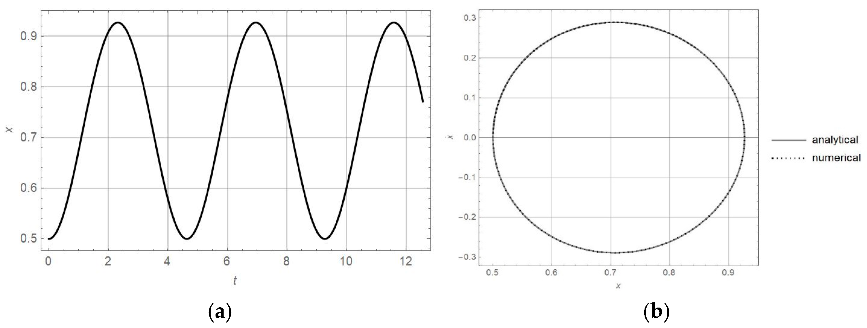
For the initial conditions $\mathrm{x}\left(0\right)=0.5$, $\dot{\mathrm{x}}\left(0\right)=0$, the second-order differential Equations (57) and (58) are solved, and the obtained results are compared with the closed-form analytic solutions $x_{\mathrm{\alpha }=1}=\mathrm{ca}\left(1,1,t\right)$, and $x_{\mathrm{\alpha }=3}=\mathrm{ca}\left(3,1,t{\displaystyle \frac{\sqrt{2}}{2}}\right)$. In Figure 1a,b, the x-t diagrams obtained numerically and analytically are plotted. The numerical solutions are obtained by applying the Wolfram Mathematica 11. Comparing the x-t curves, it is obtained that the amplitudes of vibration for both oscillators are equal and that their periods of vibration differ; the period is shorter for $\alpha =1$ than for $\alpha =3$. The exact values of periods of vibration computed analytically according to (48) are

$$T_{\alpha =1}=2B\left({\displaystyle \frac{1,}{2}}, {\displaystyle \frac{1}{2}}\right)=2{\displaystyle \frac{\mathsf{\Gamma }\left(\frac{1}{2}\right)\mathsf{\Gamma }\left(\frac{1}{2}\right)}{\mathsf{\Gamma }\left(1\right)}}=2\pi =6.283,$$

(59)

$$T_{\alpha =3}={\displaystyle \frac{2B\left(\frac{1,}{4}, \frac{1}{2}\right)}{0.5\sqrt{2}}}=2\sqrt{2}{\displaystyle \frac{\mathsf{\Gamma }\left(\frac{1}{4}\right)\mathsf{\Gamma }\left(\frac{1}{2}\right)}{\mathsf{\Gamma }\left(\frac{3}{4}\right)}}=14.833,$$

(60)

where $\mathsf{\Gamma }$ is the special gamma function [25]. It is obvious that the analytic results are equal to the numerically obtained ones.

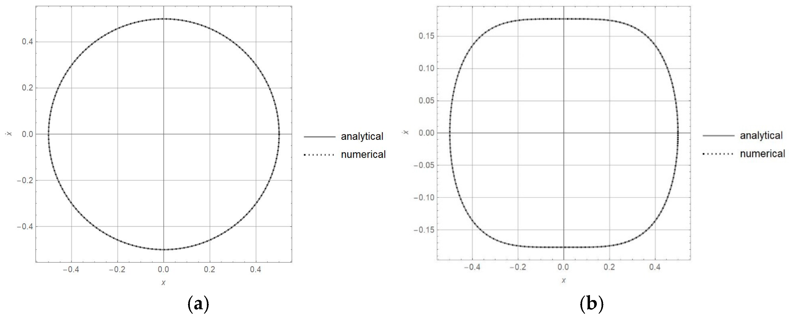
In Figure 2a,b, the $\dot{x}-x$ plots for Equations (57) and (58) are plotted. The numerically obtained curves are compared with the analytically obtained orbits ${\dot{x}}^2+x^2=0.25$ and 2${\dot{x}}^2+x^4=0.0625$, respectively. It is evident that the analytically developed result is equal to the numerically obtained one. For $\alpha =1$, the orbit is a circle with a radius of 0.5.

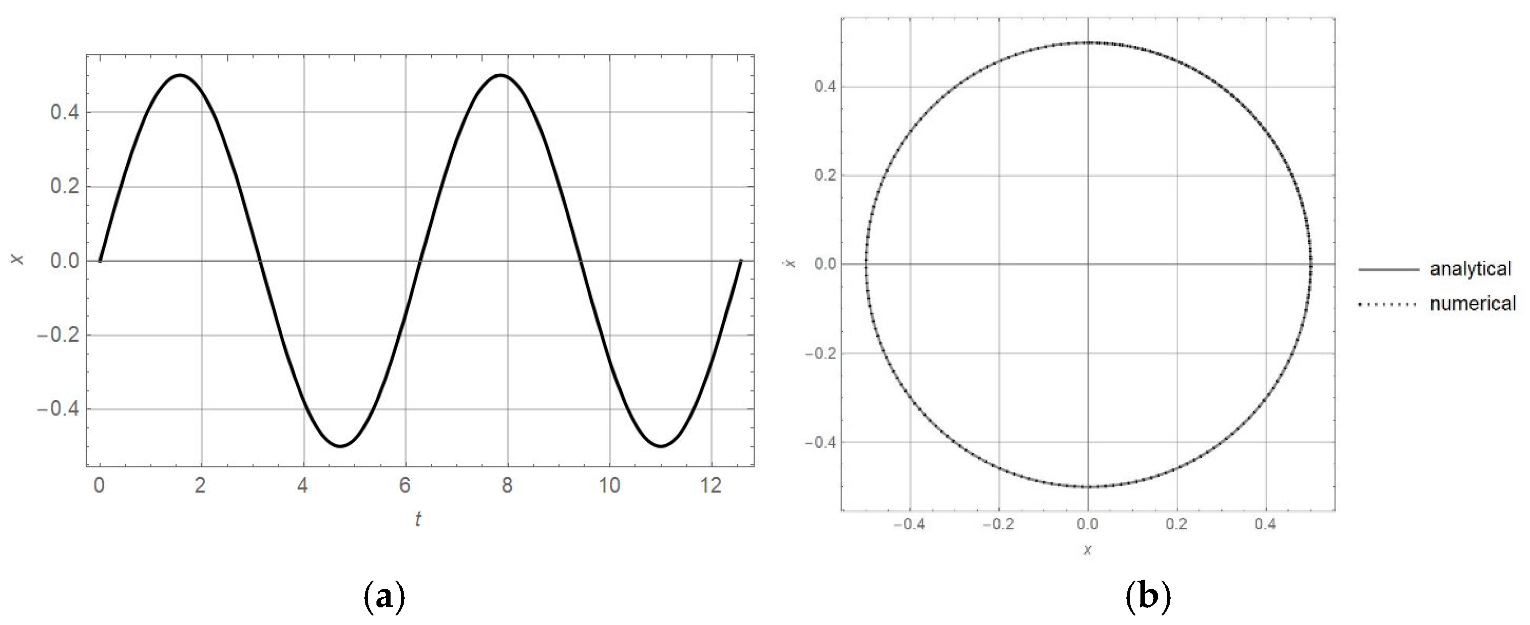
Let us consider the oscillator given with Equation (57) and the corresponding first integral for initial conditions x(0) = 0 and $\dot{x}\left(0\right)=0.5$. In Figure 3a, the x-t diagram is plotted, and in Figure 3b, the $\dot{x}-x$ diagram is plotted.

Comparing Figure 1a and Figure 3a, it is obvious that both solutions have the amplitude A = 0.5, and the oscillation is around the position $x=0.$

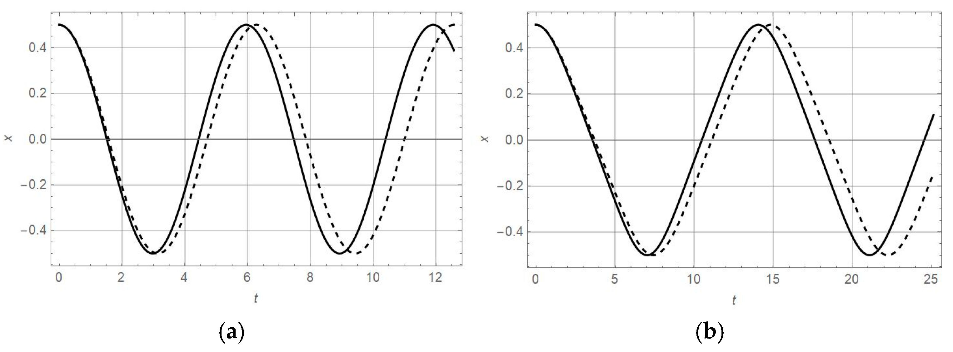
5.1. Asymptotic Solution

Let us consider the case when the parameter of nonlinearity is perturbed in comparison to that in Equations (57) and (58)

$$\left(\mathrm{a}\right) \alpha =1: \ddot{x}\left(1+x\right)+x\left(1.1+1.5x\right)+0.5{\dot{x}}^2-0.125=0,$$

(61)

$$\left(\mathrm{b}\right)\alpha =3:\ddot{x}\left(1+x\right)+x^3\left(1.1+1.25x\right)+0.5{\dot{x}}^2-0.015625=0.$$

(62)

For the initial conditions x(0) = 0.5, $\dot{x}\left(0\right)=0$, $\mathcal{F}$ = 0.5., and according to (30), the approximate analytic solutions of (61) and (62) are

$$\left(\mathrm{a}\right)x=0.5\mathrm{ca}\left(1,1,1.05t\right)\left(\mathrm{b}\right)x=0.5\mathrm{ca}\left(3,1,0.728t\right)$$

(63)

In Figure 4a, the solutions of (57) and (61) for $\alpha =1$ are plotted, and in Figure 4b, the solutions of (58) and (62) for $\alpha =3$ are plotted. Comparing the approximate solution with the numeric one, it is evident that the difference is negligible. In addition, comparing the diagrams in Figure 4a and in Figure 4b, respectively, it is obtained that the amplitude of vibration for oscillators is 0.5, while the frequency of vibration of these oscillators differs. Namely, the periods of vibration for oscillators (57) and (58) are (59) and (60), respectively, while for (61) and (62), according to (31), they are

$$(\mathrm{a})T_{\alpha =1}={\displaystyle \frac{2B\left(\frac{1,}{2}, \frac{1}{2}\right)}{{\omega }_{a1}}}=5.952, (\mathrm{b})T_{\alpha =3}={\displaystyle \frac{2B\left(\frac{1,}{4}, \frac{1}{2}\right)}{{\omega }_{a3}}}=14.401$$

(64)

Comparing the values, it is evident that the periods (64) of the perturbed Equations (61) and (62) are shorter than the periods of Equations (57) and (58).

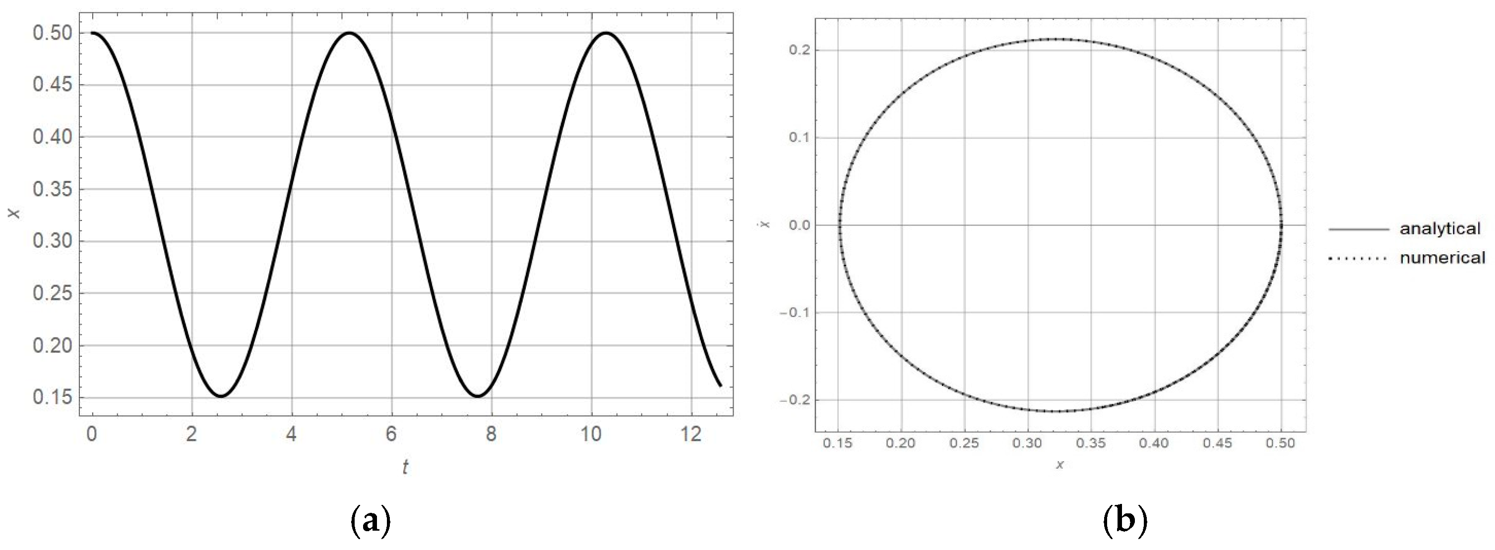
5.2. Influence of the Excitation Force

During the operation of the sieve, there is the possibility of change of intensity of the excitation $\mathcal{F}$. The influence of the force $\mathcal{F}$ on the vibration is tested. The equation of motion for the oscillator with α = 1 and ${\mathrm{c}}_{\mathrm{\alpha }}=1.5$ is

$$\ddot{x}\left(1+x\right)+x\left(1+1.5x\right)+0.5{\dot{x}}^2-\mathcal{F}=0.$$

(65)

For the initial conditions $x\left(0\right)=0.5$, $\dot{x}\left(0\right)=0$, the corresponding first integral is

$$\dot{x}=\pm \sqrt{{\displaystyle \frac{1}{1+x}}\left(0.375-x^2-x^3-2\mathcal{F}\left(0.5-x\right)\right)}.$$

(66)

Unfortunately, there is no exact analytic solution for (65). For $\mathcal{F}$ = 0.5, the x-t diagram, obtained by numeric solving of (66), is plotted (Figure 5a). In addition, in Figure 5b, the orbital motion in the $\dot{x}-x$ plane is presented. Using the relation (66) and the condition $\dot{x}=0$, it is computed that ${(x_{\dot{x}=0})}_1=0.15$ and ${(x_{\dot{x}=0})}_2=0.5$ (see Figure 5b). Thus, the oscillation is around $x_{\mathrm{m}}={\displaystyle \frac{{(x_{\dot{x}=0})}_1+{(x_{\dot{x}=0})}_2}{2}}=0.325$ with amplitude $A={\displaystyle \frac{{(x_{\dot{x}=0})}_1-{(x_{\dot{x}=0})}_2}{2}}=0.175$. The analytically calculated values agree with the numerically calculated ones (see Figure 5).

The procedure is repeated for the constant excitation $\mathcal{F}$ = 1.5. In Figure 6a, the x-t diagram is plotted, and in Figure 6b, the $\dot{x}-x$ diagram is plotted. Using (66) and the condition $\dot{x}=0$, the following values are obtained: ${(x_{\dot{x}=0})}_1=0.5$ and ${(x_{\dot{x}=0})}_2=0.927$. The oscillation is around $x_{\mathrm{m}}={\displaystyle \frac{{(x_{\dot{x}=0})}_1+{(x_{\dot{x}=0})}_2}{2}}=0.7135$ with amplitude $\mathrm{A}={\displaystyle \frac{{(x_{\dot{x}=0})}_1-{(x_{\dot{x}=0})}_2}{2}}=0.2135$.

Analyzing (66), it is obvious that for $\mathcal{F}=0.375$, the numeric values are ${(x_{\dot{x}=0})}_1=0$ and ${(x_{\dot{x}=0})}_2=0.5$. The oscillation is around ${\mathrm{x}}_{\mathrm{m}}=0.25$ with amplitude $A=0.25$. According to (66), the limit value excitation is computed. Thus, for $\mathcal{F}=0.875$, the amplitude of vibration decreases to zero, and the motion is around the value ${\mathrm{x}}_{\mathrm{m}}=0$.

5.3. Mass Variation

According to the aforementioned results, the mass variation is analyzed. Using the solutions of Equations (58) and (59) for $\mathcal{F}=0.125$, the mass variation is as follows:

$$\alpha =1:\hspace{1em}\hspace{1em}m\left(t\right)=1+0.5\mathrm{ca}(1,1,t)$$

$$\alpha =3:\hspace{1em}\hspace{1em}m\left(t\right)=1+0.5\mathrm{ca}(3,1,0.707t)$$

For both sieves, the mass variation is in the interval from $m_{\min }=0.5$ to $m_{\max }=1.5$. However, the period of mass variation is longer for $\alpha =3$ than for $\alpha =1$.

In

Table 2. Mass variation for various values of excitation $\mathcal{F}$.

$\mathcal{F}$	0.125	0.375	0.50	0.875	1.500
mmin	0.5	1.0	1.15	1.5	1.500
mmax	1.5	1.5	1.50	1.5	1.927
Δm = mmax − mmin	1.0	0.5	0.35	0.0	0.427

, the mass variation as the function of the excitation $\mathcal{F}$ in the oscillator with $\alpha =1$ is shown.

The interval of mass variation decreases with the increase of $\mathcal{F}$ up to the value $\mathcal{F}=0.875$. By further increase of $\mathcal{F}$, the mass interval increases.

Generalizing the obtained results, it is concluded that for a constant excitation force of the sieve, the interval of mass variation is constant—with the same minimal mass and maximal mass boundary values. However, the time period of mass variation differs; it depends on nonlinear properties of the sieve. The higher the order of nonlinearity of the sieve, the longer the mass variation period. This result is important in designing the new sieve; namely, depending on the requirement of the time period necessary for mass variation in the process, the appropriate nonlinear sieve properties are chosen.

On the other hand, it is shown that in the existing sieve, the variation of the excitation force causes a change in the oscillatory motion and in the mass variation function. Namely, the excitation force is the control parameter for mass variation. Changing the excitation, we may obtain the appropriate mass variation prescribed to give the high efficiency of the system. This result is suitable for practical application.

6. Conclusions

The following is concluded:

• In general, the Liénard oscillator, modeled with a strong nonlinear differential equation with quadratic nonlinearity, has no closed-form analytic solution. Only for certain parameters, which depend on the initial amplitude of vibration and order of nonlinearity, does the Liénard equation have the exact solution. The analytic solution has the form of the cosine Ateb function. In spite of the fact that the damping is of quadratic order, the motion is periodical, with constant amplitude and period.
• For this type of Liénard equation, the first integral exists. Solving this integral, the period of vibration of the oscillator is obtained. The period of vibration depends on the initial amplitude and order of nonlinearity. The higher the order of nonlinearity, the longer the period of vibration.
• Analyzing the first integral, it is obtained that for various but certain initial conditions, the orbital motion of the oscillator in the phase plane is equal.
• The Liénard oscillator is the appropriate model for the sieve where the mass is varying with the position of the system. Applying the first integral, the amplitude and level of vibration of the sieve is computed. The effect of the excitation force on the sieve operation is also obtained. Increasing the excitation force up to a limit value, the interval of mass variation decreases, but with further increase of the force, the mass variation interval increases.

Future research should be oriented toward the extended and modified versions of the Liénard oscillators, with the aim to yield new insights in nonlinear phenomena and also new applications. These models with strong nonlinear damping and stiffness would allow investigation of limit cycles, bifurcations, and chaotic dynamics in various systems: electrical and signal processing, robotic actuators, mechanical, but also biomechanical and biological (neural systems, for example).