Solving Logistical Challenges in Raw Material Reception: An Optimization and Heuristic Approach Combining Revenue Management Principles with Scheduling Techniques

Abstract

The cost of transportation of raw materials is a significant part of the procurement costs in the forestry industry. As a result, routing and scheduling techniques were introduced to the transportation of raw materials from extraction sites to transformation mills. However, little to no attention has been given to date to the material reception process at the mill. Another factor that motivated this study was the formation of large waiting queues at the mill gates and docks. Queues increase the reception time and associated costs. This work presents the development of a scheduling and reception system for deliveries at a mill. The scheduling system is based on Trucking Appointment Systems (TAS), commonly used at maritime ports, and on revenue management concepts. The developed system allocates each delivery to a timeslot and to an unloading dock using revenue management concepts. Each delivery is segmented according to its priority. Higher-segment deliveries have priority when there are multiple candidates to be allocated for one timeslot. The developed scheduling system was tested on a set of 120 daily deliveries at a Portuguese paper pulp mill and led to a reduction of 66% in the daily reception cost when compared to a first-in, first-out (FIFO) allocation approach. The average waiting time was also significantly reduced, especially in the case of high-priority trucks.

1. Introduction

The transportation of raw materials in forest operations is of high importance, whether at the strategic, tactical, or operational level [1,2]. Among all means of transportation, trucks are preferred over trains or other means of transportation [3]. Inefficiencies in forest operations arise primarily from the lack of scheduled arrival times by transport companies, leading to idle periods followed by congestion when the number of trucks exceeds the port’s processing capacity [3,4].

Some studies have developed Truck Appointment Systems (TAS) as a means to minimize discrepancies between preferred and assigned arrival times [5,6]. Other studies have used revenue management to address the issue of over-planned deliveries [7], or have outlined principles for conducting simulations using revenue management concepts [8]. However, none of the available studies have addressed the combination of these methodologies in the reception of materials in forest operations, nor have they addressed the problem of long queues.

This work develops a model for creating routes and schedules, incorporating backhauling to increase efficiency. This project identifies the allocation of deliveries to time slots as a promising candidate for revenue management methods. Specifically, it employs quantity-based revenue management due to the heterogeneous “consumer” base and the allocation of limited resources (docks). Deliveries are differentiated by five factors used to calculate their priority level, followed by segmentation and allocation to docks and time slots based on these priorities. The goal is to minimize the extra cost of reception, with higher-priority deliveries incurring higher waiting costs than those with lower priority levels.

In this article, a literature review is presented in Section 2. Section 3 provides the problem description. Section 4 details the methodology and mathematical model. Section 5 describes the case study, dataset, and scenarios. Section 6 presents the results. Lastly, in Section 7, the conclusions and a discussion are provided.

2. Literature Review

The transportation of goods involves moving materials from suppliers to their final destination, accounting for about one-third of total logistics costs [9]. In the forestry sector, this cost can exceed 45% of operational expenses, highlighting the critical importance of raw material transport in this industry [1]. At the operational level, transport planning involves decisions about product flows, storage, and vehicle routing and scheduling [10]. Daily product quantities, storage locations, and delivery schedules are central considerations. While trucks, trains, and ships are used in forestry, trucks remain the most common due to their flexibility and mobility, especially for temporary harvest sites [10]. Operational plans vary by company—some use load quotas or fixed schedules, while others rely on a single transport company for planning [4].

Optimization models, such as the one developed by [4], address transport issues, including backhauling to reduce empty trips. Although the authors of [10] offer various models and heuristics for routing and scheduling, these do not differentiate between product types or supply chain complexities, indicating a gap for further exploration.

Like the challenges of forest operations, unplanned deliveries at seaports often result in severe logistical inefficiencies [11]. To address these issues, Truck Appointment Systems (TASs) have been developed and can be classified into Individual Appointment Systems (IASs) and Block Appointment Systems (BASs) [5]. IASs allocate a single delivery per timeslot, while BASs assign multiple deliveries, reducing delays and no-shows. Originally developed for medical appointments, BASs were later adapted for truck scheduling at seaports, with studies evaluating their performance under various delay scenarios. The authors of [12] adapted a model for the implementation of scheduling trucks at seaports, with different scenarios of the percentage of delayed arrival. These percentages help evaluate the model’s performance and identify which factors have a higher weight in the final solution.

Research in [5] highlights the potential of TASs to minimize discrepancies between preferred and assigned arrival times, thereby reducing congestion and improving processing efficiency. Similarities between seaport congestion and raw material reception at wood transformation centers suggest that TASs could also be effectively applied in the forestry sector. Both scenarios involve resource limitations, dual processing stages (gate and docks), and comparable delivery times, making TASs a promising solution for managing congestion in wood processing facilities Quota-regulated systems, like the one proposed for the Hong Kong port, which allocates a maximum number of deliveries per 30 min timeslot to manage spatial constraints and optimize equipment usage [6].

The application of revenue management, also known as yield management, has significantly expanded across various industries in recent years [13,14,15]. The authors of [15] distinguish between quantity-based and price-based revenue management. Quantity-based revenue management leverages consumer heterogeneity, segmenting consumers into classes and prioritizing their allocation to resources when resources are limited. Price-based revenue management, on the other hand, involves adjusting prices to manage demand. For instance, the authors of [13] explored the use of revenue management concepts in container ship slot booking, identifying factors that make these approaches suitable for transportation challenges and reviewing prior applications. To overcome the challenges of over planning, for example, Continental Airlines reported revenue increases of 15–18% from its revenue management model by implementing such an approach based on an estimated 4% no-show rate [7]. Furthermore, the authors of [8] outlined principles for conducting simulations using revenue management concepts.

In

Table 1. Summary of a literature review on scheduling systems at seaports.

Article	Objective	Decision	Solution Method
[5]	Delay Cost Minimization	Allocation to timeslot	----
[6]	Penalties Minimization	Definition of the number of slots per timeslot	-------
[11]	Truck number maximization served by timeslot	Definition of the number of slots per timeslot	Heuristic
[12]	Cost Minimization	IAS—Duration of the timeslot; BAS—Number of slots within each timeslot	----
[16]	Cost Minimization	Allocation and ideal duration of time slots	Heuristic
[17]	Waiting Time Minimization	Number of slots in each time-window	Heuristic
[18]	Cost Minimization	Allocation of time slots to deliveries	Exact
This work	Daily Reception Cost Minimization	Allocation of deliveries to time slots at delivery docks	Heuristic

, we present a summary of a literature review on scheduling systems at seaports based on their objective, decision-making, and solution method.

3. Problem Description

Our study considers the process of raw material transportation and reception at paper pulp mills. Due to the intrinsic nature of these types of raw materials, it is crucial that they are quickly transported from extraction sites to their destination. Several factors create such necessity: the rapid degradation of raw materials, security risks such as wildfires, a lack of storage space at extraction sites, and difficulty in accessing those extraction sites during certain periods of the year. The Europac Kraft pulp and paper factory in Viana do Castelo, an active transformation center since 1993 and part of the Europac Group, serves as the contextual basis for our investigation.

At the beginning of each day, a big influx of trucks is detected both at the extraction site as well as at transformation centers (paper pulp mills). The enters, like the one in Vi-ana do Castelo, expect delivery time of less than an hour; however, due to this big influx generating traffic jams and long queues, delivery time is increased to several hours. This poses a problem for the efficiency of the supply chain, as higher delivery times increase the costs of transportation. As noted in [1], transportation costs represent a big portion of procurement costs in this type of industry. As such, trying to reduce such costs is a key objective.

Additionally, increased delivery times also impact the remaining actors along the supply chain, creating a snowball effect, as transportation companies are not able to com-ply with the agreed routes and delivery times. A lack of planning at reception centers undermines scheduling operational tasks at the docks. It is therefore challenging to un-load directly at the production lines, which would be ideal, as this would increase the current processing capacity of trucks at the docks and mitigate traffic jams.

This project aims to develop a two-stage solution to the previously described congestion problem. The first stage seeks to improve the planning of daily delivery times and overcome the aforementioned challenges. Here, we apply decision variables which indicate if a particular truck is allocated to a certain timeslot at a dock. This aspect of our work enables us to reduce inefficiencies in delivery times by creating a more structured schedule.

The second stage picks up on this improved planning and proposes solutions that al-low direct unloading to occur at production lines, rather than at stockyards. The solution model provides several priority levels, allowing for the differentiation and prioritization of cargo based on importance. More significant loads are given priority, offering a strategic method to minimize transportation costs and improve economic performance. These levels also motivate transportation companies to communicate their arrival time and type of cargo, as not sharing this information can translate into high waiting times. In

Table 2. Model Parameters.

Input Data
$V$	$\mathsf{\nu }=\mathrm{1,2},\dots V;$ $V$$\mathrm{is} \mathrm{the} \mathrm{number} \mathrm{of} \mathrm{trucks} \mathrm{corresponding} \mathrm{to} \mathrm{planned} \mathrm{deliveries} \mathrm{including} V^N$ for unplanned deliveries
$D$	$d=1, 2\dots D;D$$—\mathrm{Number} \mathrm{of} \mathrm{Unload} \mathrm{locations}, \mathrm{including} \mathrm{production} \mathrm{lines} D^L$$\mathrm{and} \mathrm{stockyard} \mathrm{cells} D^S$
$T$	$t=\mathrm{1,2},\dots T;T$—Available time slots, including $T^G$ for available time slots at gates and $T^D$ for available time slots at docks
$L^G$	Time slots duration at gate (min)
$L^D$	Time slots duration at docks (min)
$d^a$	Open hour at docks (in hours and min, such as 19:25)
$d^f$	Closing hour at docks (in hours and min, such as 19:25)
$g^a$	Open hour at gates (in hours and min, such as 19:25)
$g^f$	Closing hour at gate (in hours and min, such as 19:25)
$L_{gd}$	$\mathrm{Travelling} \mathrm{time} \mathrm{from} \mathrm{gate} g$$\mathrm{to} \mathrm{docks} d$(min)
$t_d$	$\mathrm{Type} \mathrm{of} \mathrm{product} \mathrm{accepted} \mathrm{at} \mathrm{dock} d$(natural numbers)
$C^e$	Waiting time cost (€/min)
$C^m$	Cost of moving raw material within transformation centers (€/ton)
Parameters for priority method
$n$	Number of segments for classifying planned delivery
$\pi$	Percentage of available time slots which are left unused/free to handle non-planned delivery lines.
${\lambda }_i$	$\mathrm{Weight} \mathrm{of} \mathrm{used} \mathrm{criteria} \mathrm{in} \mathrm{the} \mathrm{calculation} \mathrm{of} \mathrm{priority} \mathrm{index} i=\mathrm{1,2}\dots I$$\mathrm{where} I$ is the number of priorities
${\gamma }_{1,}{\gamma }_{2, \dots }{\gamma }_{n-1}$	Limit of segments priority
$\alpha$	Acceptable delay/advance for on-time delivery (min)
$\mathsf{\Delta }$	Maximum delivery delay that does not lower segmentation (min)
${\delta }_1$	Priority weight used for recalculation of the index of delay priority
Others
$A_v^{real}$	$\mathrm{Arrival} \mathrm{time} \mathrm{of} \mathrm{truck} \mathsf{\nu }$(in hours and min, such as 19:25)
$A_v^{plan}$	$\mathrm{Arrival} \mathrm{planned} \mathrm{time} \mathrm{of} \mathrm{truck} \mathsf{\nu }$(in hours and min, such as 19:25)
$U_{vtd}^{plan}$	$\mathrm{Initial} t$$\mathrm{of} \mathrm{unload} \mathrm{at} \mathrm{dock} d$ planned $\mathrm{to} \mathrm{deliver} \mathrm{truck} \mathsf{\nu }$(in hours and min, such as 19:25)
$U_{vtd}^{real}$	$\mathrm{Initial} t$$\mathrm{of} \mathrm{unload} \mathrm{at} \mathrm{dock} d$ $\mathrm{to} \mathrm{deliver} \mathrm{truck} \mathsf{\nu }$(in hours and min, such as 19:25)
$t_{\nu }$	$\mathrm{Type} \mathrm{of} \mathrm{product} \mathrm{transported} \mathrm{by} \mathrm{truck} \mathsf{\nu }$
$p_{\nu }$	$\mathrm{Load} \mathrm{of} \mathrm{truck} \mathsf{\nu }$(ton)
$c_{\nu td}$	$\mathrm{Allocation} \cos \mathrm{t} \mathrm{of} \mathrm{delivery} \mathsf{\nu }$$\mathrm{at} \mathrm{timeslot} t$$\mathrm{at} \mathrm{dock} d$(€)

we define our model parameters.

By implementing these strategies, our work aims to provide a comprehensive solution to the longstanding and complex issues in raw material transportation and reception, presenting a new wave of innovation in industry of raw material operations/logistics.

4. Methodology and Mathematical Model

The planning of daily delivery times involves two primary phases. The first phase, which takes place the day before delivery (Del-1), focuses on scheduling deliveries to prevent an overlap. As such, on Del-1, the scheduled deliveries are booked and are temporarily allocated to a timeslot at the docks and a delivery plan is developed. The second phase, occurring on the day of delivery (Del), prioritizes the reallocation of time slots based on the discrepancy between the expected delivery time and delays. Non-scheduled deliveries are assigned specific time slots during this phase.

4.1. Stage 1—Arrival Time Planning and Timeslot Allocation (Del-1)

As previously mentioned, the first step involves calculating the priority level of each delivery. Subsequently, the deliveries are distributed across the gate ($T^G$) and dock $\left(T^D\right)$ time slots based on the priority value obtained. This step is carried out as follows:

• Calculation of priority and segmentation of all deliveries in the list of planned deliveries.
• Assignment of an arrival time at the gate according to the priority of each delivery.
• Calculation of the reception cost for deliveries for all possible time slots and docks (a delivery can only be assigned to docks that handle the type of product being transported and to time slots starting after its arrival at the docks).
• Assignment of a timeslot and dock to each delivery based on a cost-minimization criterion.

The initial priority value ($P_v$) is a weighted sum of several criteria (${\sigma }_i^v$). These factors are:

• Historical delivery information—data related to the punctuality of planned arrival times from the truck’s previous deliveries to the processing center.
• Number of additional deliveries on the same day—a truck can perform multiple deliveries on the same day. This results in trucks making more than one delivery being given higher priority to ensure they have enough time to complete all their deliveries. The value for this criterion decreases with each delivery the truck completes and corresponds to the number of remaining deliveries (e.g., for a truck with three planned deliveries, the value for this criterion would be 2 for the first delivery, 1 for the second, and 0 for the final delivery).
• Delivery characteristics—these include the origin of the delivery, whether the truck transports the maximum possible load, and whether the type of product being transported is acceptable for the production lines. These factors are binary (0 or 1). For example, if the truck carries the maximum load, this factor assumes a value of 1; otherwise, it is 0.

Each of these criteria has a weight (${\lambda }_i$) in the final priority value. The criteria weight value ranges between 0 and 1.

After calculating the priority of each delivery, they are classified into segments. The segments are defined by constants (${\gamma }_{n-1}$, where $n$ is the number of adopted segments). These constants represent the minimum value from which a delivery is classified into the next priority segment. Equation (1) represents the formula used for calculating the priority of each delivery:

$$P_v={\sum }_i{\lambda }_{i }{\sigma }_i^v, {\sum }_i{\lambda }_{i }=1, 0\le {\lambda }_{i }\le 1$$

(1)

After calculating the priority of each delivery, a planned arrival time is assigned based on the desired arrival time and segment. Upon receiving the list of planned deliveries, each delivery has the desired arrival time. However, planned and desired arrival times may not coincide with the start of a timeslot, and overlapping arrivals may occur.

Deliveries are segmented into gate time slots according to their desired arrival times. Subsequently, arrival times are assigned based on each delivery’s segment. Deliveries in higher segments experience less disruption (the difference between desired and assigned arrival times), while those in lower segments are assigned times farther from their desired arrival times.

Next, a timeslot and dock are assigned to each delivery. This involves an optimal allocation aimed at minimizing the additional daily reception cost of the planned deliveries in time slots $tϵT$ and docks $dϵD$. This process can be approached using integer programming, where the decision variable $x$ assumes the value of 1 if truck $v\in V$ is allocated to timeslot $tϵT$ and dock $dϵD$ and 0 otherwise.

Decision Variable:

$$x_{vtd}=\left\{\begin{array}{c}1, \mathrm{if} \mathrm{truck} v \mathrm{is} \mathrm{allocated} \mathrm{to} \mathrm{timeslot} tϵT \mathrm{and} \mathrm{dock} dϵD \hfill \\ 0, \mathrm{otherwise}\hfill \end{array}\right.$$

The objective function is:

$$\min y={\sum }_{v\in V}{\sum }_{d\in D}{\sum }_{t\in T}{c}_{vtd}{x}_{vtd}$$

(2)

Model Constraints:

$${\sum }_{d\in D}{\sum }_{t\in T}{x}_{vtd }= 1, \forall v\in V$$

(3)

$${\sum }_{v\in V}{x}_{vtd }\le 1, \forall t\in T, \forall d\in D$$

(4)

$${\sum }_{v\in V}{\sum }_{d\in D}{\sum }_{t\in T}{x}_{vtd}\le (1-\pi )$$

(5)

$$x_{vtd} \in \left\{\mathrm{0,1}\right\}, \forall v\in V, \forall t\in T, \forall d\in D$$

(6)

Objective function (2) reduces the total cost of receiving raw materials through the optimal allocation of planned delivery arrival times to available time slots and docks. The objective function which calculates the total cost is constructed as a sum of products of binary variable $x_{vtd}$ and the cost coefficients ($c_{vtd}$) ($v=\mathrm{1,2}\dots V, t=\mathrm{1,2}\dots T, d=\mathrm{1,2}\dots D$). The cost function calculates the extra reception cost caused by inefficiencies in the supply chain.

The remaining equations form the constraints of the model. Equation (3) ensures that each delivery must be assigned to exactly one timeslot. In this problem, it is assumed that unloading operations start at the beginning of each timeslot and that the truck is empty by the end of it. To achieve this, the duration of the unloading period (timeslot at the docks) corresponds to the maximum duration of the unloading operation. Conversely, each timeslot at a given dock can be assigned to at most one delivery (Equation (4)).

The next constraint limits the number of deliveries assigned to production line $\pi$ time slots to ensure availability for unplanned deliveries (Equation (5)). At this initial stage, it is expected that most deliveries will be allocated to production line time slots, but it is not mandatory for all of them to be.

Due to long waiting times or limitations imposed by Equation (5), some planned deliveries may end up being allocated to the stockyard. Finally, Equation (6) forces the variables to be binary.

$$W_v=U_{vtd}^{real}-(A_v^{real}+L^G+L_{gd})$$

(7)

Equation (7) represents the calculation of the total waiting time ($W_v$) which is used in Equation (8) for cost calculation. The total waiting time is the difference between the start time of unloading operations $\left(U_{vtd}^{real}\right)$ and the arrival time at the processing centre $\left(A_v^{real}\right)$, including the time taken to process the delivery at the gate and the travel time between the gate and the docks.

The factors included in this cost calculation are the waiting time for each delivery to be processed at the gate and subsequently at the docks. Additionally, the function considers the cost of moving raw materials from the stockyard to the production lines. Both components are weighed by the priority level of each delivery to prioritize the allocation of more critical deliveries. The cost of labor for the gate and docks during regular working hours is not included in the cost function.

Each cost coefficient is calculated using the following formula in Equation (8).

$$c_{\nu td}={\displaystyle \frac{C^e{W}_v+C^m{p}_{\nu }}{P_v}}, \forall v:t_v=t^d, t=\mathrm{1,2}\dots T^D$$

(8)

The first component of the cost formula is the product of the total waiting time ($W_v$) and the unit queue waiting cost ($C^e$). The waiting cost for gate processing is always zero, because the planned arrival time for each delivery ensures that there are no overlapping arrivals. The waiting cost ($C^e$) is defined as the average fixed cost for a loaded truck specializing in each type of raw material.

The second component concerns the cost of moving goods within the processing center. This component is only considered when unloading is performed at the stockyard rather than directly at a production line. The movement cost is calculated as the product of the unit movement cost ($C^m)$ and the load transported by the truck ($p_{\nu }$). At this initial stage, it is not necessary to include overtime labor costs at the processing center, as planned deliveries are distributed to be handled within regular working hours. For equal values of the components in Equation (8), timeslot $t$ is assigned to the delivery with higher priority.

The calculation of the initial priority of each delivery ($P_{\nu }$) in Equation (1) establishes an inverse relationship between priority and cost, implying that the higher the value of ${(P}_{\nu })$, the lower the cost $(c_{\nu td}$), and vice versa. Consequently, if the product transported is not accepted at dock $d$, the cost will be higher.

4.2. Stage 2—Real Allocation of Deliveries (Del)

The second stage takes place on the day of the deliveries (Del). In this stage, the final allocation of planned deliveries, along with unplanned ones, is carried out. The algorithm implemented in the second stage is presented below:

• Calculation of the revised priority and segmentation accordingly;
• Computation of the waiting queue at the gate (addition of new arrivals to the existing waiting queue);
• Assignment of a timeslot at the gate to the best candidate in the waiting queue;
• Computation of the waiting queue at the docks (addition of new arrivals to the existing waiting queue);
• Allocation of time slots at the docks to the best candidates for each type of product;
• Verification of the stopping condition (when the timeslot at the gate exceeds the closing hour and there are no deliveries in the waiting queue). If true, stop; otherwise, return to step 1.

The first step of this stage involves calculating the revised priority for each delivery based on delays. The delay for each delivery is determined as the difference between the scheduled arrival time and an index that marks deliveries arriving on time. This index is normalized by the gate’s closing hour. The calculation of this index is based on tolerance parameter $\alpha$. The aforementioned parameter establishes the tolerance window around the scheduled arrival time in which a delivery is considered on time (e.g., if the tolerance is 5 min, a delivery with a scheduled arrival time of 07:10 is considered on time if it arrives between 07:05 and 7:15).

The delay is then used to calculate the revised priority ($P_v^u$). The revised priority, together with the revised segment thresholds, is used to reclassify the deliveries based on their delay.

$$\varphi =\min \{\left(A_v^{plan}+\alpha \right);\left(U_{vtd}^{plan}-L_{gd}-L^G\right)\}$$

(9)

$$L_v=\left\{\begin{array}{c}{\displaystyle \frac{A_v^{real}-\varphi }{g^f}}, if A_v^{real}>\varphi \\ 0, otherwise \end{array}\right.$$

(10)

$$P_v^u={\delta }_{1 }{P}_v+{\delta }_{2 }\left(1-L_v\right), { \delta }_{1 }+{\delta }_{2 }=1;0\le { \delta }_{1 }, {\delta }_{2 }\le 1$$

(11)

$${\gamma }_n^u={ \delta }_{1 }{\gamma }_n+{\delta }_{2 }\left(1-{\displaystyle \frac{\mathsf{\Delta }}{g^f}}\right)$$

(12)

The delay for each delivery is given by Equation (10). The value of this function depends on the result of Equation (9), which corresponds to the index marking deliveries that arrive on time. If the actual arrival time ($A_v^{real}$) is later than the index, the delivery is considered late, and the delay must be calculated. Otherwise, the delay is set to zero. Once the delay is calculated for each delivery, the revised priority index ($P_v^u$) is determined using Equation (11).

With the changes in priorities, it also becomes necessary to create new threshold levels for each segment. These new threshold values are calculated using Equation (12).

At this stage, four segmentation levels now exist. In addition to the previous levels (low, medium, and high), a very-low priority level is introduced. The downgrading process is controlled by the downgrade parameter ($\mathsf{\Delta }$). This parameter represents the delay threshold beyond which a delivery at the lower limit of a segment is downgraded to the next lower segment (e.g., a delivery initially classified with a priority level of 0.6 in the high-priority segment will be downgraded if its delay is equal to or exceeds 30 min). For higher delays, deliveries in lower priority levels are downgraded, while those in higher priority levels retain their segment. Even deliveries in the highest priority segment can be downgraded to lower levels when significant delays occur. Unplanned deliveries have a revised priority ($P_v^u$) equal to zero and are classified in the very low priority segment.

The process of updating priorities and segments is dynamic and occurs as deliveries arrive at the transformation center.

The second and third steps of this stage operate almost as a single process and are represented by Figure 1. Step 2 involves computing the new waiting queue at the gate. This is achieved by adding new arrivals, which occur between the end of the previous timeslot and the beginning of the current one, to the existing queue. Then, the best candidate in the waiting queue is selected based on the following criteria: delay relative to the scheduled time, segment, and arrival time. The first criterion for selecting the best candidate is the delay. If one or more planned deliveries have zero delay in the waiting queue, they take priority over all others. If there is only one delivery with zero delay, the timeslot at the gate is automatically assigned to that delivery. The second criterion is the segment. If there are multiple deliveries with zero delay, or if none exist, the candidates are divided by their respective segments. As expected, deliveries classified in a higher segment take priority over others. If multiple deliveries exist in the same segment, the tie-breaking criterion is the arrival time at the transformation center.

Once processed at the gate, the trucks proceed to the docks which we can see in Figure 2. At the docks, the allocation process for time slots is like that used at the gate. Deliveries arrive at the docks and are classified according to the timeslot in which they arrive. Then, the deliveries are divided by the type of product they are carrying, since the docks for each product type are independent. After this division, the allocation process for time slots and docks begins.

If a product type has only stockyard dock as the unloading location, the allocation process works the same way as at the gate. Deliveries are initially divided into those with and without delays. If only delayed deliveries exist or if multiple deliveries have zero delay, the segment criterion is applied, and if necessary, the real arrival time criterion is also used.

If a product type has both production lines and stockyard docks as unloading locations and there are multiple deliveries in the waiting queue, the allocation process becomes more complex. In this case, it is necessary to verify the number of deliveries that a specific product type will have in the following timeslot and to determine whether the waiting cost is lower than the cost of moving raw materials from the stockyard to the production lines.

The list of deliveries for a specific product in the upcoming timeslot is determined in phases. First temporary allocations are considered in the first stage. Then we look at the deliveries processed at the gate with arrival time at the docks between the start of the current timeslot and the start of the next.

Two situations can arise:

• If the number of deliveries in the next timeslot is less than the number of available production lines for a specific product type, it is possible to assign one of the deliveries to a production line in the next timeslot. In this case, it is necessary to check whether the waiting cost is lower than the cost of moving the delivery with the smallest weight to the next timeslot. If the waiting cost is lower, the lower-priority delivery remains in the waiting queue. Conversely, if moving the goods is less expensive, the delivery with the smallest weight is assigned to the stockyard, and the rest are assigned to production lines.
• If the number of deliveries is equal to or exceeds the number of available production lines, all deliveries are assigned to docks in the current timeslot, as the same situation would occur in the next timeslot if a delivery were left waiting.

The process of allocating time slots is immediate and can occur at the start of each timeslot.

5. Case Study, Scenarios and Dataset

5.1. Case Study

The proposed solution method was tested in a raw material reception scenario at a transformation center. The case was based on the Europac Kraft pulp and paper factory of the Europac Group in Viana do Castelo. The Europac Group is the fourth-largest producer of kraftliner for paper and cardboard products. The group operates 30 transformation centers across Portugal, Spain, and France. The Viana do Castelo center has been active since 1993, producing approximately 350,000 cubic meters of paper annually. For paper production, it consumes around 700,000 cubic meters of maritime pine and about 180,000 cubic meters of eucalyptus. Most of the raw materials consumed are sourced from domestic suppliers, with a small portion coming from the group’s own production.

Wood is transported to the Viana do Castelo center by road using specialized trucks. Each truck carries only one type of product, with no mixing allowed at any stage of the transport or reception process. The maximum capacity is limited by national regulations to between 28 tons and 48 tons [19]. The transportation of raw materials is outsourced to third parties.

Currently, the reception of raw materials is conducted without any planning, with all deliveries being unplanned. A medium-sized transformation center can receive approximately 120 deliveries per day, with the process following the workflow described in Section 4.

Operations at the gate take less than 10 min. The load is weighed and directed to a discharge dock based on its characteristics. There is a designated storage area (stockyard) for each type of accepted product. The unloading operation takes between 10 and 15 min and is performed using a crane. At the end of this operation, the truck is weighed again to calculate the delivery value. The operation of supplying production lines occurs throughout the workday (10 to 14 h per day). Internal movement of raw materials is carried out using the transformation center’s fleet, which increases total operating costs.

The current method applied in the service stage and the unloading stage is the FIFO method. This method, combined with the lack of delivery planning, makes it impossible to perform direct unloading onto the production lines, as previously mentioned.

5.2. Scenarios Created

An important difference between the scenarios analyzed is whether deliveries are planned. Booking involves receiving a list of planned deliveries on the day prior to their execution and distributing them throughout the day, allocating a timeslot at the gate to avoid overlapping deliveries. This process also includes the temporary assignment of a timeslot at a dock where raw materials are to be unloaded. Processing deliveries during the booking phase depends on the methodology applied in the scenario being analyzed. For scenarios without booking, all deliveries are unplanned, resulting in many overlapping arrivals.

We have created four different scenarios to analyze:

• FIFO (unplanned): The baseline method, which serves as the point of comparison, is the simple FIFO scenario, in which all deliveries are unplanned. In this scenario, as the booking phase or priority-based reception is not applied, the lack of planning means that deliveries can only be unloaded into the stockyard.
• FIFO (planned): After distributing deliveries throughout the day, delays are calculated based on the difference between the planned arrival time and the actual arrival time. In this model, it was established that planned deliveries can be unloaded both onto production lines and in the stockyard, whereas unplanned deliveries can only be unloaded in the stockyard.
• Priority (unplanned): In this case, the dataset used is the same as in the FIFO scenario with unplanned deliveries, but the processing of deliveries is handled differently. In this model, all deliveries can be unloaded either onto production lines or in the stockyard.
• Priority (planned): The final scenario corresponds to the combination of the developed priority-based model, that is, booking of time slots and docks in the first stage, followed by the final allocation according to the priority level in the second stage.

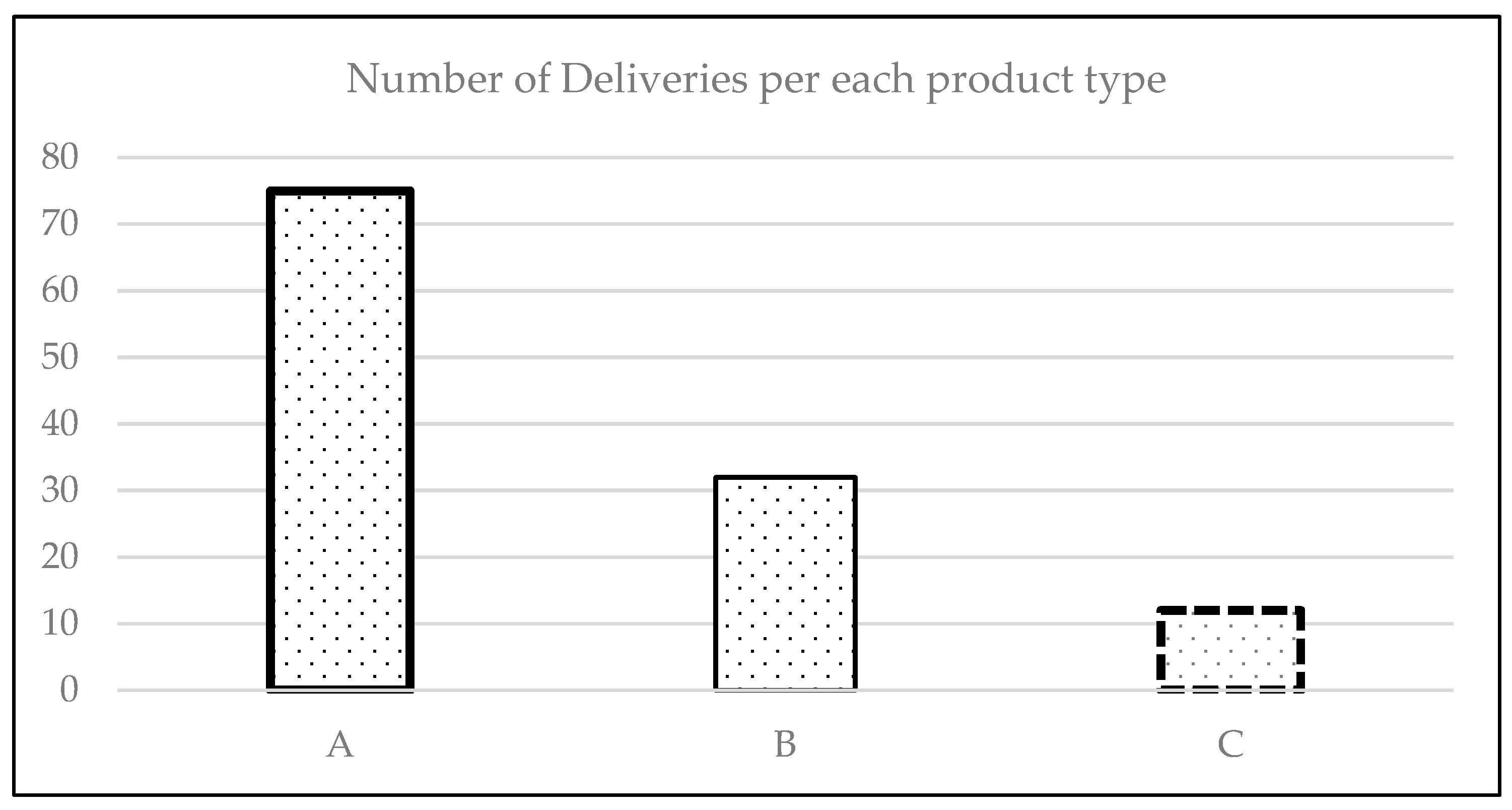
5.3. Dataset

5.3.1. General Dataset

The dataset analyzed pertains to a single day of deliveries at the transformation center under study. This center is divided into two key areas: the gate, where deliveries are processed upon arrival, and the docks, where trucks unload their transported materials. The operating schedule is organized into 2 h time windows, which are further subdivided into 7 min and 15 min time slots.

At the unloading area, three types of products are accepted: eucalyptus with bark (Type A), eucalyptus without bark (Type B), and maritime pine (Type C). Each product type has designated unloading points. Products of Type A are associated with two production lines and one dock in the stockyard. Type B products have one production line and one stockyard, while Type C products are linked to a single stockyard. The allocation of docks is based on the proportion of deliveries for each product type. In Figure 3, we present the distribution of each type of product per number of deliveries.

The dataset contains details on each truck’s preferred arrival time, cargo, and product type. Additionally, the planned delivery data include information essential for calculating priority levels, such as historical delivery behavior, the number of additional deliveries a truck will make on the same day, and the origin of the delivery. Planned deliveries comprise 72 entries, created from real-world data. Of these, 40% are marked as coming from market suppliers. Trucks with multiple deliveries on the same day are identified using an attribute that tracks the remaining deliveries for that truck (e.g., for a truck with three deliveries, the attribute decreases from 2 to 1 to 0 for subsequent deliveries).

The distribution of deliveries per time window and within those windows was generated randomly. However, to reflect real-world conditions, 40% of deliveries were scheduled to arrive during peak hours (09:00–11:00, 11:00–13:00, and 19:00–21:00), when the number of arrivals exceeds the processing capacity of the gate and docks.

Unplanned deliveries represent 40% of the total and are classified as having very low priority in the priority methodology. Their arrival times are random and not controlled, which means they may occur outside the center’s working hours. Deliveries that arrive before opening wait to be processed, while those arriving after closing are processed at the gate, but only stockyards are available at the docks.

To replicate real-world scenarios more accurately, delays were incorporated into the models with booking (planned), causing the actual arrival times to often differ from the planned arrival times. Approximately 54% of deliveries arrived late, while 24% arrived early; only 22% arrived on time.

The final dataset reflects a single day of operations at the transformation center, encompassing 120 deliveries. These are divided into 57 from forests (48 of which are unplanned), 57 from extraction sites, and 14 from market suppliers.

5.3.2. Reception Dataset

The transformation center operates from 6:00 to 21:00, with activities at the gate starting at 6:00 and at the docks at 7:00. The schedule is divided into 2 h time windows, with the gate using 7 Min time slots ($L^G)$ and the docks using 15 min time slots ($L^D$), corresponding to the maximum truck unloading time. The average transit time between the gate and docks is 10 min ($L_{gd}$).

Docks are divided into production lines and stockyards. Unloading directly at production lines is prioritized as it allows immediate use of materials, whereas unloading stockyards incurs additional costs of 0.35 € per ton ($C^m$) to move materials to production lines. Waiting time also has a cost of 0.51 € per minute ($C^e$), making it economically advantageous to wait for a production line spot if the waiting time does not exceed a cost threshold.

Under the FIFO methodology, direct unloading at production lines is not allowed, forcing all trucks to unload at the stockyards. However, the proposed heuristic allows for direct unloading at production lines unless the waiting time exceeds the threshold, making the system more cost-efficient. For instance, a truck carrying 30 tons will wait for a production line spot unless the waiting time surpasses 20.5 min, beyond which unloading at the stockyard becomes the preferable option.

Table 3. Constant Values applied to model.

Constant	Value
Input Data:
$D$	= {1,2,……6}
V	= {1,2……120}
$L^G$	= 7 min
$L^D$	= 15 min
$g^a$	= 360 (corresponds to 06:00)
$d^a$	= 420 (corresponds to 07:00)
$d^f, g^f$	= 1260 (corresponds to 21:00)
$L_{gd}$	= 10 min
$t^d$	$=t^1=t^2=t^4=\left\{A\right\}, t^3=t^5=\left\{B\right\};t^6=\left\{C\right\}$
$C^e$	= 0.51 €/min
$C^m$	= 0.35 €/min
Parameters for model
$n$	3 (low, medium and high priority)
$\pi$	10%
${\lambda }_i$	${\lambda }_1=0.5; {\lambda }_2=0.2; {\lambda }_3={\lambda }_4={\lambda }_{5 }=0.1$
$\gamma$	${\gamma }_1=0.6; {\gamma }_2=0.3$
$\alpha$	4 min
$\mathsf{\Delta }$	30 min
${\delta }_1$	0.5

lists all constant values applied to the model, i.e., both input and parameters.

5.3.3. Priority Model Parameters

During the initial phase, booking time slots at the gate and temporarily assigning deliveries to time slots at the docks require parameters for the weight of each priority component and limits for each segment. The model includes five parameters in the priority formula:

• ${\sigma }_1^v$—Historical performance of the last 15 deliveries.
• ${\sigma }_2^v$—Number of remaining deliveries to be completed by the truck.
• ${\sigma }_3^v$—Match between the transported product and the products accepted by the production lines.
• ${\sigma }_4^v$—Delivery originating from a priority source (e.g., maritime ports).
• ${\sigma }_5^v$—Truck carrying a maximum load.

Weights for these criteria in the priority formula are: ${\lambda }_1=0.5; {\lambda }_2=0.2; {\lambda }_3={\lambda }_4={\lambda }_{5 }=0.1$. The priority value of each delivery ranges between 0 and 1.

The segmentation of each delivery is determined by its priority value. After priority calculation, segment limits are used for the classification of deliveries into segments. During the booking phase, deliveries are categorized as low, medium, or high priority (n = 3 priority levels).

The segment limits are as follows:

• Deliveries with priority values below 0.3 are classified as low priority.
• Deliveries with priority values between 0.3 and 0.6 are classified as medium priority.
• Deliveries with priority values above 0.6 are classified as high priority.

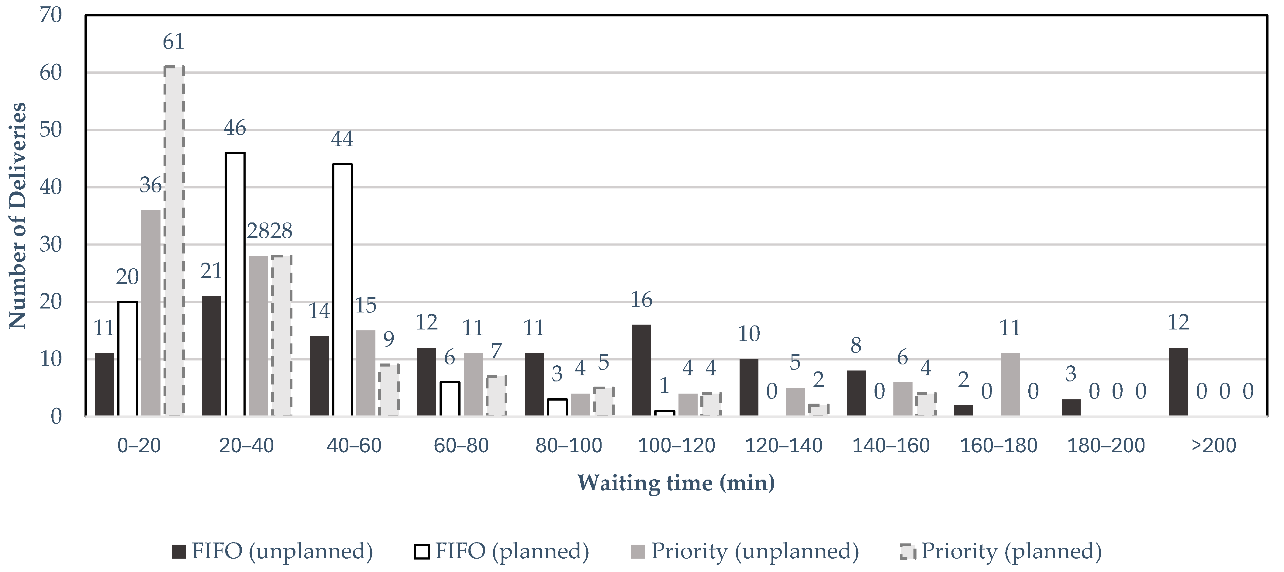
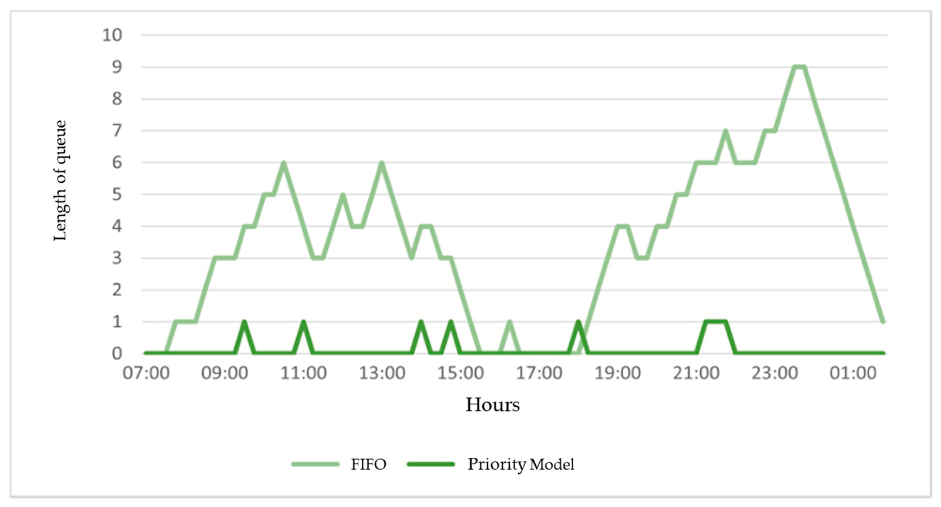
When the booking of an additional parameter ($\pi$) is considered, a value of 10% is applied.

On the delivery day, the final allocation of deliveries to time slots occurs. This stage incorporates unplanned deliveries and delays in planned deliveries. In the case study analyzed, tolerance parameter ($\alpha$) is set to 4 min. Deliveries arriving within 4 min of their scheduled time are classified as having a delay of zero.

To calculate the new priority level, two factors are considered: the initial priority and the delay. These are weighted equally, with parameters 1 and 2 each assigned a value of 0.5. Regarding segments, an additional classification level is introduced at this stage, resulting in four segments: low, medium, high, and very low priority. All unplanned deliveries are classified as very low priority. Planned deliveries with significant delays may also be downgraded to this classification. The downgrade of planned deliveries is based on the parameter $\mathsf{\Delta }$, which is set to 30 min.

6. Results

To perform calculations and present results, the Gurobi optimizer was used; the data were run using an Intel 5 processor. In the following sections we will present three types of results: cost indicators, time indicators and allocation indicators.

6.1. Cost Indicators Results

The results obtained in this section indicate the additional reception cost incurred in each of the evaluated scenarios. The costs are divided into waiting costs at the gate, waiting costs at the docks, and the cost of moving goods between the stockyard and the production lines.

Regarding the waiting costs at the gate, it is possible to observe that the models yield identical costs depending on whether the model includes booking or not. The models incorporating booking (FIFO planned and priority planned) exhibit a gate waiting cost of 1589.67 €, while the remaining models (FIFO unplanned and priority unplanned) show a cost of 3287.97 €. As such, we can deduce that booking implementation offers significant economic advantages, reducing gate reception costs by approximately 52%. Although FIFO models yield similar values to the priority models, it is important to note that FIFO models do not segment deliveries. As such, FIFO models fail to prioritize more critical deliveries. In the analysis of all the indicators, it is possible to conclude that the bottleneck in the reception process is at the gate. The gate incurs higher waiting costs than the docks in all the developed models.

For waiting costs at the docks, the results vary more across scenarios. A quick analysis shows that the baseline model, FIFO (unplanned), incurs the highest additional dock reception cost. This can be explained by the fact that, in this scenario, unloading is only possible at the stockyard due to the lack of delivery planning. Consequently, this model also experiences the highest cost of moving goods between the stockyard and the production lines.

With the implementation of the booking phase in the FIFO model, it becomes possible to unload some deliveries directly at the production lines. In this scenario, planned deliveries can be unloaded at both the lines and the stockyard, while unplanned deliveries are restricted to the stockyard. This ability to unload at the lines significantly reduces the waiting cost for unloading, reaching levels even lower than those in the priority model without booking. The reduction in stockyard unloading also leads to a decrease in movement costs of goods, as expected.

In the priority model (unplanned), it is possible to unload all deliveries at both locations (stockyard and production lines). However, it is observed that the dock reception cost in this scenario exceeds that of the FIFO model (planned). This is partly explained by the stockyard reception cost. In the FIFO model (planned), allocating all unplanned deliveries to the stockyard alleviates the waiting queue at the production lines, resulting in lower waiting costs. Conversely, in the priority model (unplanned), deliveries are only allocated to the stockyard when the movement cost exceeds the waiting cost for a slot at the lines in the next timeslot.

Finally, in the priority model (planned), deliveries can be allocated to both the lines and the stockyard, like the previous model. However, in this scenario, the distribution of planned deliveries throughout the day results in lower dock costs compared to the other models. Additionally, this model minimizes the cost of moving goods.

After comparing all models, significant gains are achieved with the implementation of the priority model (planned). This model enables a reduction in total reception costs by approximately 66% compared to the baseline model (FIFO unplanned) and by about 21% compared to the FIFO model with reservation. While the cost reduction compared to FIFO (planned) scenario may not initially seem highly significant, it should be noted that this model does not process deliveries based on their priority segments.

From the analysis of gate reception costs, it can be concluded that booking implementation provides significant economic benefits, reducing costs from 3287.97 € to 1589.67 €, as shown in

Table 4. Cost Indicators Results.

Cost (€)	FIFO (Unplanned)	FIFO (Planned)	Priority (Unplanned)	Priority (Planned)
Gate	3287.97	1589.67	3287.97	1589.67
Docks	2482.17	702.27	715.02	488.07
Total Waiting Time	5770.14	2291.94	4002.99	2077.74
Movement	1317.40	671.65	371.00	270.20
Total	7087.54	2963.59	4373.99	2347.94

.

6.2. Time Indicators Results

Time-related indicators are associated with the waiting time for each delivery. The waiting time for each delivery is divided into waiting time at the gate and waiting time at the docks. This analysis calculates the average waiting time at the gate and docks, the average waiting time per delivery, and the maximum waiting time for a delivery.

As seen from the analysis in

Table 5. Time Indicator Results.

Waiting Time (min)	FIFO (Unplanned)	FIFO (Planned)	Priority (Unplanned)	Priority (Planned)
Medium at gate	53.73	25.98	53.73	25.98
Medium at Docks	40.56	11.48	11.68	7.98
Medium Delivery	94.28	37.45	65.41	33.95
Maximum from delivery to delivery	280.00	105.00	240.00	158.00

, the average waiting times at the gate are identical for the two planned models and the two unplanned models. The results for the average waiting time at the gate align with those obtained for the corresponding waiting costs. As mentioned earlier, although the FIFO models yield values similar to those of the models where the developed methodology is implemented, it is important to note that FIFO models do not account for the priority of each delivery. The analysis of gate waiting times confirms that implementing a booking process on the day prior to delivery significantly contributes to delivery waiting time reduction.

Regarding the waiting time at the docks, the baseline model, FIFO (unplanned), presents the highest values. This can be explained because deliveries are allocated only to time slots at the stockyard due to a lack of planning. FIFO (planned) and priority (unplanned) models exhibit similar unloading times.

The average waiting times for each delivery demonstrate that the developed priority model (planned) is superior to the other models. The average waiting time per delivery in the priority model (planned) is approximately 63% lower than the average reception time in the FIFO (unplanned) model.

Finally, it is worth noting that the maximum waiting time in the priority model (planned) is significantly higher than the maximum value observed in the second-best model, FIFO (planned). This occurs because, in the priority model, a delivery in the lowest priority segment may need to wait for extended periods, whereas in the FIFO model, deliveries are not allocated based on their priority segments but rather according to their arrival time at the transformation center.

Figure 4 illustrates the distribution of waiting times for each delivery across the various developed models. The histogram shows that more than half of the deliveries in the priority model (planned) require 20 min or less for all operations to be completed. Conversely, in the FIFO (planned) model, most deliveries (90 deliveries) have waiting times of between 20 and 60 min. Lastly, it is also highlighted that the FIFO (unplanned) exhibits a high number of deliveries with waiting times exceeding 180 min (15 deliveries).

In Figure 5, it is possible to analyze the progression of the waiting queue at the docks throughout the day, including during overtime hours.

Another advantage of implementing the priority model (planned) is the stabilization of the waiting queue at the docks. As shown, the number of deliveries in the dock waiting queue in the priority model (planned) never exceeds 1 unit, whereas in the FIFO model, it reaches up to 9 units after the docks close.

The graph also highlights the greater number of deliveries waiting during peak hours. The peak hours occur during the time windows 9:00–11:00 and 11:00–13:00, and subsequently from 19:00 onward.

6.3. Allocation Indicators Results

This section analyzes the indicators related to the allocation of available resources (time slots at the gate and docks). To this end, the number of deliveries unloaded at the production lines and the stockyard, as well as the number of time slots provided at each location, were calculated. Additionally, the analysis includes the number of deliveries arriving at the transformation center after closing time (21:00), the number of deliveries processed at the gate after closing (gate queue), and the number of deliveries processed at the docks after closing (dock queue).

Before analyzing the resource allocation indicators, the number of extra time slots required at both the gate and the stockyard beyond the transformation center’s closing time was determined. It is important to note that after closing time (21:00), the production lines stop operating, but the stockyard and gate can continue working overtime.

Table 6. Number of extra time slots required at the gate and stockyard for all models.

	FIFO (Unplanned)	FIFO (Planned)	Priority (Unplanned)	Priority (Planned)
Gate	22	16	22	16
Stockyard	20	9	15	9

shows the number of extra time slots required at the gate and stockyard for all models.

In

Table 7. Arrival time processed after closing hours.

	FIFO (Unplanned)	FIFO (Planned)	Priority (Unplanned)	Priority (Planned)
Arrival	2	6	2	6
Processed at Gate	22	7	22	7
Processed at stockyards	31	10	26	10

, it is observed that the number of deliveries arriving late is higher in the planned models compared to the models without planning. This is attributed to delays in planned deliveries. In the reservation models, late arrivals consist of four planned deliveries and two unplanned deliveries. As expected, the number of deliveries processed at the gate is identical between paired models since the distribution of deliveries differs, but the processing approach remains unchanged. At the docks, however, the number of deliveries waiting to be processed after closing time varies across the models.

In the FIFO (unplanned) model, a higher number of deliveries wait to be processed due to its lower reception capacity compared to other models. The priority (unplanned) model, despite having double the capacity of the baseline model, still shows a significant number of deliveries awaiting processing, primarily due to the clustering of deliveries at certain arrival times. Finally, both the FIFO (planned) and priority (planned) models show 10 deliveries to be processed after closing time. The number of deliveries processed in total is the same across all models (120 deliveries), and the majority of these late arrivals are part of this total.

The occupancy rate is calculated based on the available time slots during regular hours, combined with the additional time slots required to handle deliveries arriving and queuing after closing time. To provide a more accurate analysis, the occupancy rate for production lines is calculated separately from the stockyard’s occupancy rate.

Table 8. Occupancy of available resources.

	FIFO (Unplanned)	FIFO (Planned)	Priority (Unplanned)	Priority (Planned)
Occupancy gate (%)	80.00	83.33	80.00	83.33
Occupancy lines (%)	0.00	33.33	50.00	55.95
Occupancy stockyard (%)	52.63	32.82	16.90	13.33

shows that the gate occupancy rate is similar across all models, exceeding 80.00%. In the FIFO (unplanned) model, the line occupancy rate is 0.00%, as deliveries can only be made to the stockyard in this model. In the other models, line occupancy is observed, with the highest values achieved in the priority with reservation model.

6.4. Results Summary

Based on the analysis of all the indicators, it is possible to conclude that the bottleneck in the reception process is at the gate. The gate incurs higher waiting costs than the docks in all the developed models.

The difference between reception costs at the gate and the docks is smaller in the FIFO model (unplanned), as this model only has three locations for unloading deliveries, which leads to longer queues. In the priority models, the difference in cost and waiting time between the gate and the docks becomes significantly more pronounced since, in these models, the reception capacity at the docks is much higher than at the gate.

Finally, it can be observed that the occupancy of time slots at the gate is also much higher than the occupancy of time slots at the docks.

The developed priority (planned) model shows substantially better results compared to the other models, with reception costs being 52% lower than the base model and a waiting time reduction of 66%.

7. Conclusions and Discussion

This work aimed to develop a methodology for the planning and reception of deliveries at a wood processing center.

Firstly, an analysis of the current reception process at the processing center was conducted. In the initial model, all deliveries were unplanned, which made it impossible to plan arrivals in a way that would reduce waiting times. With this model, the processing center incurred an additional daily reception cost of 7087.54 €.

Subsequently, a new delivery management methodology was developed based on the application of revenue management concepts. Existing literature revealed that the reception of deliveries at seaports shares many logistical similarities with the present case study. In the analyzed cases of congestion at seaports, it was observed that implementing a planned system led to significant reductions in processing times for each delivery. Based on these planned systems, a system was developed for planned deliveries, allowing for the allocation of deliveries to time slots and docks the day before they are executed, with the aim of reducing the extra reception cost.

For the allocation of deliveries to time slots, revenue management concepts were used. This process involves segmenting deliveries into priority levels and subsequently allocating them to time slots based on their priority. Deliveries classified in higher segments have more time slots available for allocation and take precedence over deliveries in lower segments. The planning of some deliveries enables them to be unloaded directly onto production lines, leading to significant reductions in waiting times and, consequently, in reception costs.

On the day of delivery execution, unplanned deliveries are added, and their allocation to time slots is based on the priority criterion. Delivery planning also reduces raw material handling costs within the processing center, as direct unloading onto production lines becomes possible.

The applied methodology led to monetary gains of approximately 66% compared to the currently used method. This was achieved due to the significant reduction in the average reception time for each delivery. Besides the financial advantages for the processing center, delivery planning also benefits the carrier. With minimal planning, the carrier could reduce the number of trucks needed for operations and lower overtime costs for workers.

Efficient communication between carriers and the processing center is essential for the functioning of the developed reservation system.

The developed model could benefit from the implementation of tracking systems for planned deliveries to monitor the delivery status. In cases where a delivery experiences significant delays, this could enable a more optimized allocation of gate time slots to trucks waiting in the queue.

In the developed model, time slots with fixed durations were implemented, regardless of the type and quantity of transported goods. Due to the lack of prior control and insufficient data about the process, it was impossible to conduct a more in-depth study of the optimal duration for each timeslot. As a result, the maximum duration of the unloading process was adopted, which generates idle time when the process takes less than 7 min at the gate and less than 15 min at the docks.

References

1. Palmgren, M.; Rönnqvist, M.; Värbrand, P. A near-exact method for solving the log-truck scheduling problem. Int. Trans. Oper. Res. 2004, 11, 447–464. [Google Scholar] [CrossRef]
2. Malladi, K.; Sowlati, T. Optimization of operational level transportation planning in forestry: A review. Int. J. For. Eng. 2017, 28, 198–210. [Google Scholar] [CrossRef]
3. Carlsson, D.; Rönnqvist, M. Backhauling in forest transportation: Models, methods, and practical usage. Can. J. For. Res. 2007, 37, 2612–2623. [Google Scholar] [CrossRef]
4. Rönnqvist, M. Optimization in forestry. Math. Program. 2003, 97, 267–284. [Google Scholar] [CrossRef]
5. Abdelmagid, A.; Gheith, M.; Eltawil, A. A Binary Integer Programming Formulation and Solution for Truck Appointment Scheduling and Reducing Truck Turnaround Time in Container Terminals. In Proceedings of the 2020 7th International Conference on Industrial Engineering and Applications, Bangkok, Thailand, 16–21 April 2020. [Google Scholar]
6. Murty, K.; Wan, Y.; Liu, J.; Tseng, M.; Leung, E.; Lai, K.-K.; Chiu, H. Hongkong International Terminals Gains Elastic Capacity Using a Data-Intensive Decision-Support System. Interfaces 2005, 35, 61–75. [Google Scholar] [CrossRef]
7. Gorin, T.; Brunger, W.; White, M. No-show forecasting: A blended cost-based, PNR-adjusted approach. J. Revenue Pricing Manag. 2006, 5, 188–206. [Google Scholar] [CrossRef]
8. Frank, M.; Friedemann, M.; Schröder, A. Principles for simulations in revenue management. J. Revenue Pricing Manag. 2008, 7, 7–16. [Google Scholar] [CrossRef]
9. Buffa, F.P.; Munn, J.R. A Recursive Algorithm for Order Cycle-time that Minimizes Logistics Cost. J. Oper. Res. Soc. 1989, 40, 367–377. [Google Scholar] [CrossRef]
10. Audy, J.-F.; Rönnqvist, M.; D’Amours, S.; Yahiaoui, A.-E. Planning methods and decision support systems in vehicle routing problems for timber transportation: A review. Int. J. For. Eng. 2022, 34, 143–167. [Google Scholar] [CrossRef]
11. Huynh, N.; Walton, C. Robust Scheduling of Truck Arrivals at Marine Container Terminals. J. Transp. Eng. 2008, 134, 347–353. [Google Scholar] [CrossRef]
12. Huynh, N. Reducing Truck Turn Times at Marine Terminals with Appointment Scheduling. Transp. Res. Rec. 2009, 2100, 47–57. [Google Scholar] [CrossRef]
13. Quante, R.; Meyr, H.; Fleischmann, M. Revenue management and demand fulfillment: Matching applications, models, and software. OR Spectr. 2009, 31, 31–62. [Google Scholar] [CrossRef]
14. Kuyumcu, A.; Yildirim, U.; Hyde, A.; Shanaberger, S.; Hsiao, K.; Donahoe, S.; Wu, S.; Murray, M.; Maron, M. Revenue Management Delivers Significant Revenue Lift for Holiday Retirement. Interfaces 2018, 48, 7–23. [Google Scholar] [CrossRef]
15. Talluri, K.T.; van Ryzin, G.J. The Theory and Practice of Revenue Management; International Series in Operations Research & Management Science; Springer US: New York, NY, USA, 2005; ISBN 978-1-4020-7933-7. [Google Scholar]
16. Chen, G.; Yang, Z. Optimizing time windows for managing export container arrivals at Chinese container terminals. Marit. Econ. Logist. 2010, 12, 111–126. [Google Scholar] [CrossRef]
17. Xiaoju, Z.; Zeng, Q.; Chen, W. Optimization Model For Truck Appointment In Container Terminals. Procedia-Soc. Behav. Sci. 2013, 96, 1938–1947. [Google Scholar] [CrossRef]
18. Phan, M.-H.; Kim, K. Negotiating truck arrival times among trucking companies and a container terminal. Transp. Res. Part E Logist. Transp. Rev. 2015, 75, 132–144. [Google Scholar] [CrossRef]
19. Antram: Novo Regulamento de Pesos e Dimensões. 2017. Available online: https://antram.pt/attachments/legislacao/DL%20132-2017.pdf (accessed on 1 September 2020).
Figure 1. Second Stage—Delivery Arrival and Processing at the Gate.
Mathematics 13 00919 g001
Figure 2. Second Stage processing at docks.
Mathematics 13 00919 g002
Figure 3. Distribution of products per number of deliveries.
Mathematics 13 00919 g003
Figure 4. Histogram with the frequency of number of deliveries and waiting time for all 120 deliveries and all four scenarios.
Mathematics 13 00919 g004
Figure 5. Progression of the number of deliveries in waiting queues at the docks along the day.
Mathematics 13 00919 g005