1. Introduction
Polynomials and special functions are crucial in various fields because of their several uses in applied sciences; see, for instance, ref. [
1,
2,
3]. Many theoretical publications have been devoted to the different polynomial sequences. The authors of [
4] explored several polynomial sequences and offered a few practical uses for their findings. In ref. [
5], the authors investigated different polynomial sequences. In ref. [
6], degenerated polynomials of the Apostol type were introduced. The authors of [
7] examined Sheffer polynomial sequences. Several articles also examined certain generalized polynomials. For example, the authors of [
8] developed several other generalized polynomials. A significant subject in numerical analysis and the solution of various differential equations (DEs) is the utilization of distinct sequences. A great deal of effort has been focused on this area. For example, the authors of [
9,
10] used specific polynomials to solve some DEs, which are generalizations of the first and second kinds of Chebyshev polynomials. The generalized Bessel polynomials and the generalized Jacobi polynomials were used to address multi-order fractional DEs in [
11,
12]. The authors of ref. [
13] employed a set of generalized Chebyshev polynomials to solve the telegraph DEs.
High-order DEs are central to numerous applications in science and engineering, including structural mechanics, fluid dynamics, and electromagnetic theory. Over the past few decades, significant advancements have been made in developing efficient numerical methods to address these complex problems. Among the most notable techniques are spectral methods, which have demonstrated superior convergence properties compared to traditional finite difference and finite element methods, especially for problems with smooth solutions [
14,
15,
16].
Recent advancements in machine learning have shown promising applications in solving ODEs and PDEs. Various studies have successfully implemented machine learning techniques, providing innovative solutions and insights into complex dynamics. For instance, the work by Qiu et al. [
17] explored novel machine learning frameworks for ODEs, while Zhang et al. [
18] demonstrated effective methodologies for PDEs. Additionally, the study by Cuomo et al. [
19] highlighted the evolving role of machine learning in enhancing computational efficiency and accuracy in this domain. These contributions collectively illustrate the dynamic development of machine learning approaches in addressing differential equations and underscore the potential for further exploration in our research.
In addition to the emerging techniques in machine learning and operational calculus, it is crucial to recognize traditional numerical methods that have been extensively employed in the approximation of differential equations. For instance, Runge–Kutta methods provide a robust framework for solving ordinary differential equations, offering varying degrees of accuracy depending on the specific formulation used. Similarly, differential transformation methods have gained attention for their efficiency and ease of implementation in obtaining numerical solutions. These classical approaches have been explored in literature, as highlighted in recent studies (e.g., [
19,
20]), and will be discussed further to provide a comprehensive overview of the landscape of numerical techniques applicable to differential equations.
Heat transfer, wave propagation, fluid dynamics, and many more areas of physics and engineering extensively use PDEs. In addition, biology uses them to model population dynamics and disease transmission, while economics uses them to compute price alternatives. Photodynamic enzymes are vital in medical imaging. The geosciences utilize them for weather prediction and groundwater movement simulation, while the material sciences employ them for chemical reaction and diffusion studies. For some applications of different PDEs, see [
21,
22]. Several numerical techniques exist for solving different PDEs. For example, the authors of [
23] followed a variational quantum algorithm for handling PDEs. In [
24], some studies of an inverse source problem for the linear parabolic equation were performed.
Spectral methods use global basis functions, such as orthogonal polynomials or trigonometric functions, to approximate the solution to DEs. These methods can be classified into various types (see, for example, [
25,
26,
27,
28]). The main spectral methods are collocation, tau, and Galerkin. The collocation method relies on choosing suitable nodes in the domain and, after that, satisfying the equations at these points. Many authors use the collocation method because it is easy to implement and can handle various DEs. For example, the authors of [
29] applied a wavelet collocation approach to treat the Benjamin–Bona–Mahony equation. Another collocation approach using third-kind Chebyshev polynomials was followed in [
30] to treat the nonlinear fractional Duffing equation. In [
31], the authors applied a collocation procedure to specific high-order DEs. The collocation method treated inverse heat equations in [
32]. Some other contributions regarding collocation methods can be found in [
33,
34,
35]. The Galerkin method and its variants are also among the essential spectral methods. The main principle of applying this method is to choose basis functions that meet the underlying conditions. For example, the authors of [
36] applied a Jacobi Galerkin algorithm for two-dimensional time-dependent PDEs. Some other contributions regarding the Galerkin method can be found in [
37,
38,
39,
40]. The tau method can be applied without restrictions on the choice of basis functions. In [
41], the authors followed a tau approach for certain Maxwell’s equations. Another tau approach was followed in [
42] to solve the two-dimensional ocean acoustic propagation in an undulating seabed environment. A tau–Gegenbauer spectral approach was followed for treating certain systems of fractional integro DEs in [
43]. Some other contributions can be found in [
44,
45,
46].
Table 1 summarizes the key publications related to Galerkin’s methods for solving DEs, including the types of equations addressed, the specific Galerkin approach used, and notable findings.
In 1800, Heinrich Rothe proposed the Telephone numbers (TelNs) method while computing the involutions in a set of n elements. In a telephone system, where each subscriber may only be linked to a maximum of two other subscribers, the sequence of TelNs can alternatively be seen as the number of feasible methods to make connections between the n subscribers. In graph theory, the quantity of matchings in a whole graph with n vertices is another use of the TelNs. In this paper, we will develop a generalization for the TelNs to build a sequence of polynomials, namely TelPs. We will employ these polynomials to solve some ODEs and PDEs.
In this study, we propose a spectral Galerkin approach for solving some models of DEs. We utilize the TelPs as basis functions. We will propose suitable basis functions for handling some models of DEs. The convergence analysis for the used expansions will be discussed.
The structure of this paper is organized as follows:
Section 2 gives an overview of the mathematical properties of TelPs and develops an inversion formula, which is essential for analyzing the error analysis of the used expansion.
Section 3 describes the Galerkin formulation for the high-order linear IVPs, while
Section 4 proposes a collocation algorithm for treating the non-linear IVPs.
Section 5 extends the method to systems of DEs, while
Section 6 discusses the application to hyperbolic PDEs. In
Section 7, a comprehensive investigation of the convergence and error analysis is performed. Numerical results presented in
Section 8 validate the efficiency and accuracy of the presented methods, with concluding remarks and future research directions in
Section 9.
8. Numerical Results
Several test examples are presented in this section to demonstrate the effectiveness of the proposed algorithms. Comparisons between the results obtained using the proposed method and those from other methods show that the proposed methods are highly effective and convenient. The following examples are considered.
Example 1. Consider the linear eighth-order problem [56]subject to the conditionsand the analytical solution is . Table 2 in Example 1 displays three sets of absolute error values using the proposed methods, with different numbers of points
N (16, 20, and 24). The absolute errors decrease significantly as
N increases, indicating that the method becomes more accurate with a higher number of points. This suggests the method is effective in reducing error and improving numerical precision.
At smaller values of z (e.g., ), the errors are generally lower.
At larger values of z (e.g., ), the errors increase, indicating potential challenges in achieving high accuracy in these regions.
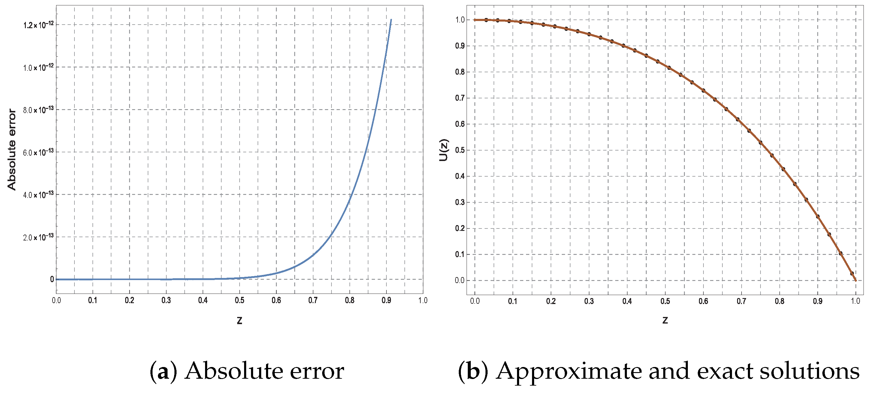
Figure 1 illustrates the corresponding absolute error function (left) and the comparison between the approximate and exact solutions (right) for Example 1 at
. The plot on the left demonstrates that the absolute error remains very small and increases gradually at
, confirming the method’s reliability and precision in solving the given problem. The plot on the right shows an excellent agreement between the approximate and exact solutions, indicating the high accuracy of the method.
Example 2. Consider the linear second-order problem (see [57])with two different sets of initial conditions and corresponding exact solutions: In each case,
is selected accordingly to satisfy the differential equation.
Table 3 presents a comparative analysis of two computational methods, Romanovski–Jacobi tau method (R-JTM) [
57] and the proposed TGM, for solving numerical Example 2. The table details each method’s absolute errors and CPU time (s) at varying numbers of discretization points
N. The results demonstrate the superior accuracy of the TGM method, achieving significantly smaller absolute errors compared to R-JTM [
57]. For instance, at
, TGM exhibits an absolute error of 8.03 × 10
−17, while R-JTM at
shows 2.96 × 10
−13. Furthermore, TGM is more computationally efficient, requiring only
seconds at
, in contrast to R-JT’s
seconds at
. The table highlights that TGM offers a better balance between accuracy and efficiency, establishing it as a more favorable choice for solving similar problems with solutions of the form
. Notably, while CPU time increases with
N in both methods, the rate of increase is substantially lower for TGM.
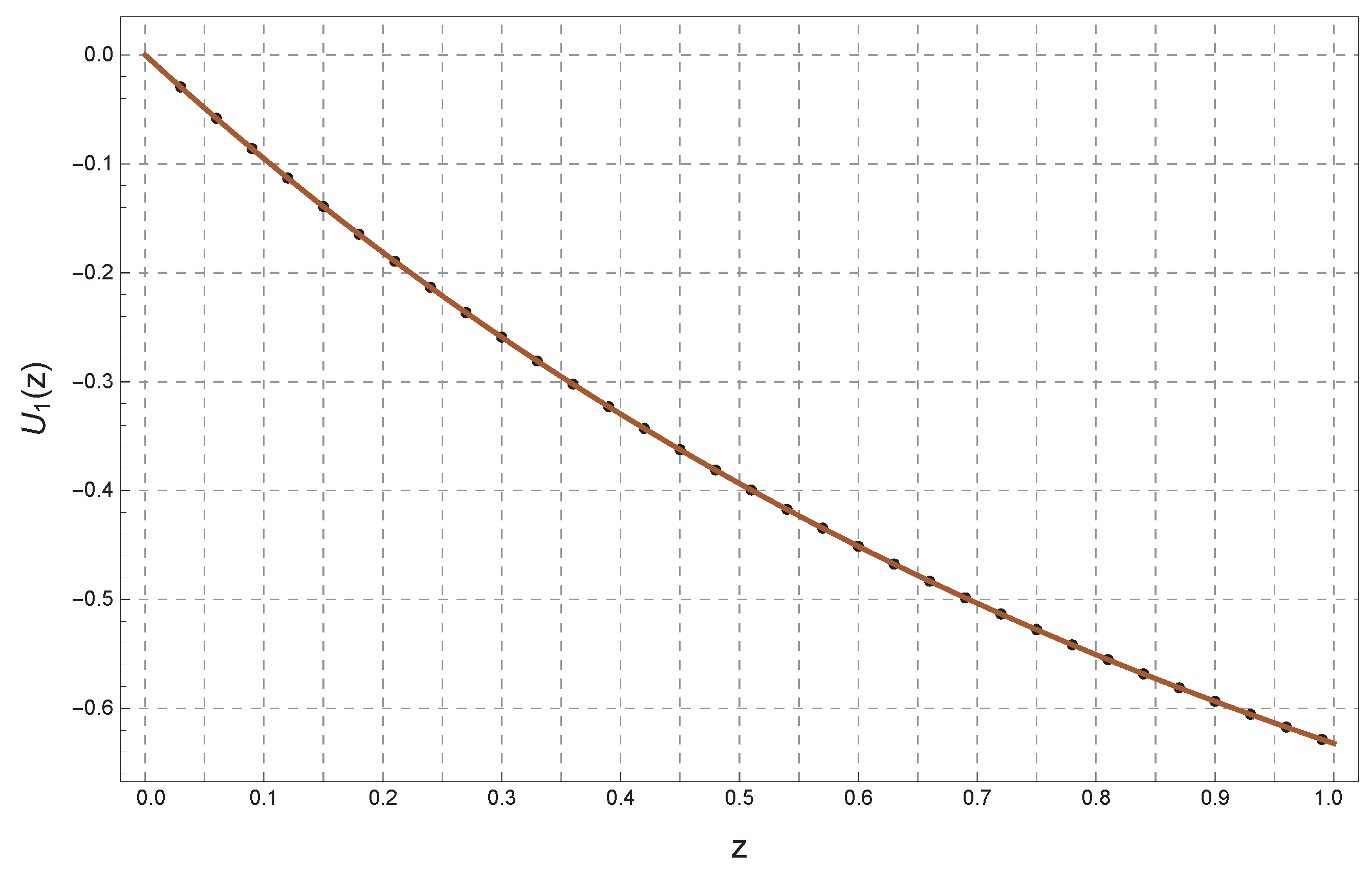
Figure 2 compares the exact solutions of a second-order differential equation in Example 2. In the left plot, the solution
is shown for
, exhibiting a smooth increasing behavior before decreasing, with a good match between the numerical and analytical solutions. In the right plot, the solution
is presented for
, displaying a more oscillatory pattern. The first solution demonstrates exponential behavior, while the second shows strong oscillatory effects. This figure highlights the possibility of obtaining different solutions for the same equation depending on the initial conditions.
Remark 4. In both accuracy and computational efficiency, the TGM approach beats the R-JTM method [57]. TGM is the better method for this problem as it requires considerably less CPU time and yields much less absolute errors. Example 3. The isothermal gas spheres equation [57] is given by the following equation:with the following initial conditions:An approximate solution to this equation, as obtained by Wazwaz [58], Liao [59], and Singh et al. [60], is given by the following formula: Table 4 presents the approximate values of
for the standard Lane–Emden equation with
, obtained using TGM. These results are compared with those derived from the Jacobi Rational Pseudospectral Method (JRPM) [
61], the variable weight fuzzy marginal linearization (VWFML) method [
62], and the Adomian Decomposition Method (ADM) solution [
58].
Example 4. We consider the following linear ODE system [63],with the ICsThe exact solution of this problem are and . Table 5 and
Table 6 provide a comparison of the absolute errors
and
for the functions
and
, solved using different methods. Here are some observations on the tables:
They show a clear difference in solution accuracy between the three methods used (Differential transformation method (DTM) in [
64], Bessel collocation method (BCM) in [
63], and the present method). The present method achieves significantly higher accuracy, with much smaller error values at the same points
.
In
Table 5, it is evident that the errors produced by the present method are much smaller compared to those of the DTM and BCM methods, especially as
N increases from 6 to 10.
In
Table 6, the present method again demonstrates notably higher precision than the DTM and BCM methods across all
points.
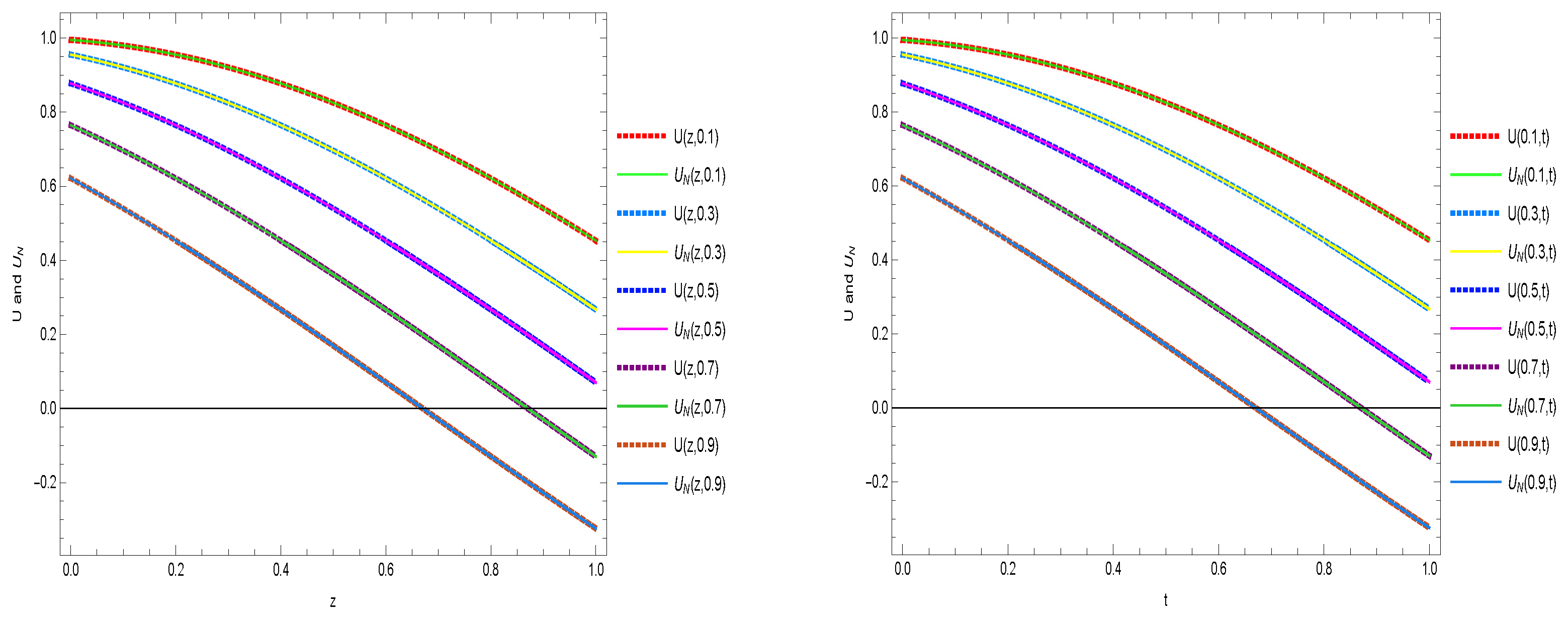
Also,
Figure 3 and
Figure 4 are plotted to compare the analytic solution with the approximate solution at
for Example 4.
Example 5. We consider the following hyperbolic equation of first-order of the form [33]subject to initial and boundary conditions,where The exact solution is given by Table 7 compares the absolute errors at various points in the
domain for Example 5, with
. The errors are shown for two previous methods (Legendre wavelets (LW) and Chebyshev wavelets (CW) from Singh et al. [
33]) and the present method.
It is notable that the errors in the present method are significantly lower compared to the LW and CW methods. For instance, at point , the error in the present method is , while the errors in the other methods are and , respectively.
This result highlights the efficiency of the present method in substantially reducing the error compared to the other methods, reflecting higher accuracy.
Table 8 compares the
errors for Example 5 at different values of
N.
It is clear that the present method shows reduced errors as the values of N increase, with the error decreasing significantly with larger N. For instance, at , the error in the present method is , while the errors in the other methods are and for the LW and CW methods, respectively.
The present method demonstrates excellent performance as N increases, achieving very high accuracy, such as at , indicating the method’s strength in convergence and accuracy.
Also,
Figure 5 compares the curves of analytical and approximation solutions for Example 5, where
, at
and
. Finally,
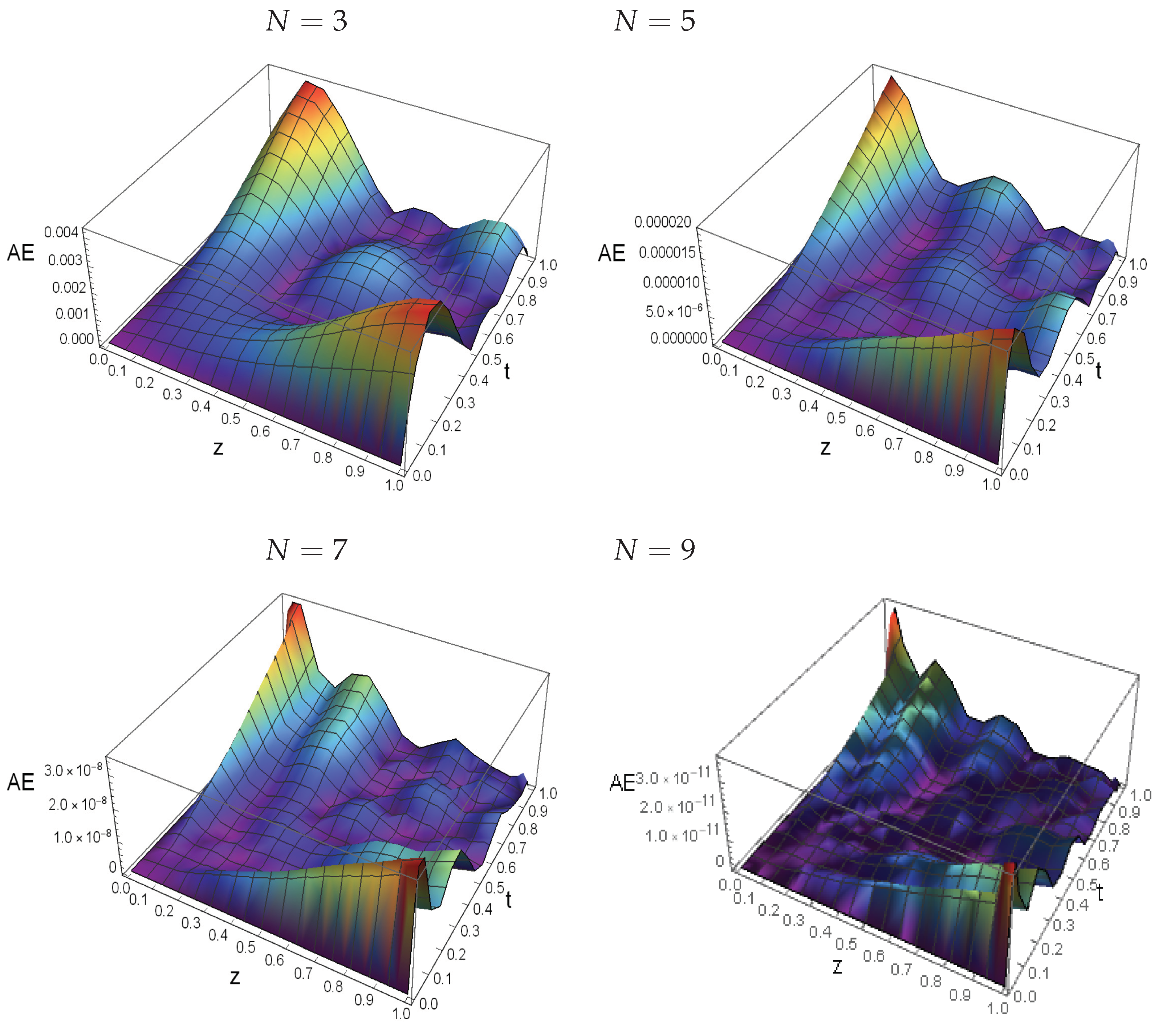
Figure 6 illustrates the space-time graphs of the absolute error functions for Example 5 at various choices of
N, specifically
,
,
, and
. The graphs depict the distribution of errors over time and space, reflecting the accuracy of the proposed method in solving the problem. It is evident that increasing the values of
N results in a significant reduction in errors, confirming the method’s effectiveness in terms of accuracy and convergence.


 ,
, 


