The Numerical Solution of an Inverse Pseudoparabolic Problem with a Boundary Integral Observation

Abstract

Direct and inverse problems for a pseudoparabolic equation are considered. The direct (forward) problem is to find the solution of the corresponding initial–boundary-value problem for known model parameters, as well as the initial and boundary conditions. The well-posedness of the direct problem is shown and a priori estimates of the solution are obtained. We study the inverse problem for identifying the flux on a part of the boundary of a rectangle, using integral measurement on the same part of the boundary. We first reduce the inverse problem to a direct one. The initial–boundary-value direct problem is with nonclassical (integrodifferential) boundary conditions. We develop a finite-difference scheme for numerically solving this problem. Numerical test examples demonstrate the effectiveness of the proposed method. It successfully handles the nonclassical integrodifferential boundary conditions and provides accurate numerical solutions.

1. Introduction

Initial–boundary-value problems for pseudoparabolic equations, also known as Sobolev-type equations [1], characterized by the presence of mixed space and time derivatives in the highest-order terms, are widely studied in the literature due to their significant applications. For instance, they can be found in the multiphase flow problem in porous media [2], filtration [3], electrical conduction phenomenon in heterogeneous media [4], two-phase porous media flows, homogeneous fluid flow in fissured rocks and the transport problems of humidity in soil [5,6], heat or mass transfer in a stably stratified turbulent shear flow [7], heat transfer in a heterogeneous medium or moisture transport in soils [8], solvent uptake in polymeric solids [9], etc. The pseudoparabolic Benjamin–Bona–Mahony equation is applicable to the study of long waves and shallow water waves, as well as drift waves in plasma or the Rossby waves in rotating fluids. Let us note that Schrödinger-type equations can describe the propagation of optical waves that include amplification, deformation, and prolongation; see, e.g., [10].

The well-posedness of a one-dimensional (1D) pseudoparabolic model is proved in [7] and the qualitative solutions behavior is also investigated. Some qualitative properties, especially the long-term dynamics of the solutions of a 1D pseudoparabolic equation, are studied in [9]. In [11], authors investigate solutions of a pseudoparabolic model over the halfstrip with two types of boundary conditions. The existence, uniqueness, and regularity of the solution is discussed in [12] for a pseidoparabolic problem. In [13], the authors consider a class of pseudoparabolic problems with integral boundary conditions. Using energy inequality, they prove the existence, uniqueness, and stability of the solution. The authors of [14] prove the local existence and uniqueness of a weak solutions of a fractional pseudoparabolic equation with singular potential. The comparison principle and new existence and nonexistence results for solutions of a nonlinear source initial–boundary-value problem for the generalized Boussinesque equation are established in [15].

The well-posedness for two pseudo-parabolic problems, connected by transmission condition through interfaces, is established in [4]. A local existence and uniqueness of a weak solution of a system of pseudoparabolic equations with Robin–Dirichlet conditions is proved in [16]. The weak solvability of a nonlinearly coupled system of parabolic and pseudoparabolic equations is discussed in [17].

Pseudoparabolic models are investigated numerically, for example in [2,5,6,8,18]. Two-dimensional (2D) nonlinear pseudoparabolic equations with Dirichlet boundary conditions are approximated by spectral schemes in space and robust schemes in time. A three-layer finite-difference scheme and a higher-order difference method for an initial–boundary-value problem for a 1D pseudoparabolic equation with time delay in the second spatial derivative, is constructed in [5,6]. An implicit finite-difference scheme for a third-order linear pseudoparabolic equation with nonlocal integral conditions is investigated in [18]. A two-grid finite-element method is presented in [19] to solve 2D nonlinear pseudoparabolic integro-differential equations. Differential and difference boundary-value problems for a third-order pseudoparabolic equation with variable coefficients and Caputo fractional derivative is studied in [8]. The authors establish results for uniqueness of the solution and stability regarding to the initial data and the right-hand side, as well as the convergence of the discrete solution to the exact one. A three-layer alternating-direction implicit scheme is studied in [20], for solving a nonlocal boundary-value problem for a 2D pseudoparabolic equation.

The solution of inverse problems is crucial in physics and engineering, as it enables the reconstruction of parameters, coefficients, source terms, boundary conditions, and initial data essential for system analysis and optimization. For instance, determining the filtration parameters, in solving environmental monitoring problems, in thermal engineering, identifying heat fluxes helps prevent overheating, while in material science, determining stress distributions ensures structural integrity. These solutions provide valuable insights into system behavior that are often unattainable through direct measurements alone or for quantities that cannot be directly measured; see, e.g., [21,22,23,24].

Inverse problems are ill-posed and it is challenging to solve them even numerically [24,25,26,27,28,29].

Inverse problems for parabolic diffusion, sub-diffusion, and similar classes of equations have been extensively investigated. In contrast, inverse problems for pseudoparabolic equations and their fractional counterparts have received comparatively less attention. Notable contributions in this area include a concise review presented in [30], which outlines key developments and provides results on the existence and uniqueness of solutions for time-fractional pseudoparabolic equations. For additional foundational studies, see, for example [9,22,31,32,33,34,35,36].

The solvability of the inverse problem of finding a solution and a time-dependent coefficient in a pseudohyperbolic equation known as the Klein–Gordon equation for given integral overspecified data is studied in [37]. The existence, uniqueness, and regularity of the solution of the inverse problem for recovering the diffusion and the leading coefficient in 2D and multi-dimensional linear pseudoparabolic equations of filtration are investigated in [35,36]. The results for the existence, uniqueness, stability of a strong generalized solution and a numerical investigation of the inverse problem for recovering space-dependent source terms in pseudoparabolic equations with memory is proposed in [31]. In [22], the Galerkin method is applied to prove the existence of the solution for the inverse coefficient problem for a third-order pseudoparabolic equation. A finite-difference method is also developed to solve the problem numerically. An inverse problem for identifying the space-dependent coefficient of the source term in a pseudoparabolic equation is studied in [32]. The authors prove the unique solvability of the problem and the stability of the solutions. The inverse problem is solved, utilizing cubic B-spline functions and reformulating the problem as a nonlinear least-squares optimization of the Tikhonov regularization functional. The existence and uniqueness of the solution and an implicit finite-difference scheme are constructed in [38] to solve an inverse source quasi-linear pseudoparabolic problem with periodic boundary conditions. In [39], the authors consider an inverse problem for determining an unknown time-dependent potential coefficient in a linear pseudoparabolic equation. They prove the uniqueness and the Lipschitz conditional stability of the problem and develop an iterative algorithm to solve it. Inverse problems for a time-fractional pseudoparabolic equations are studied in [30,40]. The results for the existence and uniqueness of the solution are provided.

Boundary-condition-identification inverse problems for parabolic equations are solved in many papers. The semigroup approach is proposed in [41] to investigate the inverse problems with unknown boundary condition in a linear parabolic equation. The uniqueness and stability results for a parabolic-boundary-condition inverse problem with an overdetermined value of the solution at a fixed point on the boundary are derived in [42]. An implicit finite-difference scheme and a decomposition method to solve the boundary-condition inverse problem is used in [43].

In [44], an inverse problem for identifying Dirichlet conditions in 2D heat equations on disjoint rectangles is solved numerically. The results for the well-posedness of the direct and the inverse problems are established. The numerical approach is based on the reduction of the 2D inverse problem to a direct-heat 1D one, using integral observation and interface conditions. The existence and uniqueness of the solution of an inverse problem for the determination of the time-dependent coefficient in the boundary source for Caputo time-fractional diffusion equation is studied in [45]. To solve the problem, a meshless method based on radial basis functions is developed. The inverse problem of the identification of non-linear boundary conditions for the time-fractional diffusion equation is solved in [46]. The existence and uniqueness of the restored function is discussed. For the numerical solution of the problem, a regularization technique is applied.

Studies that investigate inverse problems for identifying boundary conditions for pseudoparabolic equation are limited. The solvability of the inverse problems for identifying the time-dependent boundary coefficient in a Dirichlet and Robins boundary condition from integral observation is investigated in [33]. The existence and uniqueness results for a time-dependent boundary-coefficient inverse problem in a 2D pseudoparabolic equation from integral observation are obtained in [34]. In [47] is considered an inverse problem for recovering the time-dependent boundary condition in a 2D linear pseudoparabolic equation with Dirichlet–Neumann boundary conditions, from integral measurements. The well-posedness of the direct and inverse problems is discussed. By reformulating the inverse problem as a 1D direct problem and applying a substitution to address the resulting nonlocality, a numerical approach is developed. In contrast to the present study, in [47] a different equation is considered—with constant coefficients and a pseudoparabolic part (a mixed third-order derivative) with respect to the time variable and only with respect to one of the spatial variables. Moreover, the Dirichlet boundary condition is reconstructed and the integral measurements are in the whole domain. The nature of this problem allows for its reduction to the 1D case. Consequently, the approach for solving the boundary-identification inverse problem in [47] is completely different from those developed in the present investigation.

This study investigates the numerical solution of an inverse problem for a variable-coefficient pseudoparabolic equation, with a particular emphasis on reconstructing the boundary flux from integral solution measurements on the same boundary. The measured concentration of a substance’s filtration on a specified portion of the domain boundary, coupled with the corresponding medium properties, serves as supplementary information to facilitate the solution of the inverse problem.

We develop a new approach to reformulate ill-posed inverse problem to a well-posed but nonlocal direct one, and then we construct a fully implicit second order in space finite-difference approximation to solve the problem.

The remaining part of this paper is organized as follows. In the next section, we formulate direct and inverse problems. In Section 3, we establish the well-posedness of the direct problem. The reformulation of the inverse problem as a direct one is described in Section 4. Numerical methods for solving direct and inverse problems are developed in Section 5. The results from numerical test examples are proposed and discussed in Section 6. The paper is finalized with some concluding remarks.

2. The Direct and Inverse Problems

In this section, we introduce direct and inverse problems for a two-dimensional pseudoparabolic equation.

Let $T>0$, $\Omega =(0,a)\times (0,b)$, $\overline{\Omega }=[0,a]\times [0,b]$ and $Q_T=\Omega \times (0,T)$, where a, b and T are positive real numbers. We consider the pseudoparabolic equation for unknown function $u(x,y,t)$, $(x,y,t)\in Q_T$

$$\begin{array}{c}\hfill \rho (x,y){\displaystyle \frac{\partial u}{\partial t}}={\displaystyle \frac{\partial }{\partial x}}\left(c(x,y)\left({\displaystyle \frac{\partial u}{\partial x}}+\mu {\displaystyle \frac{{\partial }^{2}u}{\partial t\partial x}}\right)\right)+{\displaystyle \frac{\partial }{\partial y}}\left(c(x,y)\left({\displaystyle \frac{\partial u}{\partial y}}+\mu {\displaystyle \frac{{\partial }^{2}u}{\partial t\partial y}}\right)\right)+f(x,y,t),\end{array}$$

(1)

with the initial and boundary conditions:

$$u(x,y,0)=u^0(x,y),(x,y)\in \overline{\Omega },$$

(2)

$${\displaystyle \frac{\partial u}{\partial x}}(0,y,t)={\displaystyle \frac{\partial u}{\partial x}}(a,y,t)=0,{\displaystyle \frac{\partial u}{\partial y}}(x,0,t)=0,x\in [0,a],y\in [0,b],t\in (0,T],$$

(3)

$$-c(x,b)\left({\displaystyle \frac{\partial u}{\partial y}}(x,b,t)+\tilde{\mu }{\displaystyle \frac{{\partial }^{2}u}{\partial t\partial y}}(x,b,t)\right)=r(x,t),(x,t)\in [0,a]\times (0,T],$$

(4)

where

$$\tilde{\mu }=\left\{\begin{array}{cc}\mu >0,\hfill & \mathrm{the}\mathrm{case}\mathrm{of}\mathrm{pseudoparabolic}\mathrm{flux},\hfill \\ 0,\hfill & \mathrm{the}\mathrm{case}\mathrm{of}\mathrm{parabolic}\mathrm{flux},\hfill \end{array}\right.$$

$\rho$, c, r are given smooth functions of their arguments and

$${\rho }_1\ge \rho (x,y)\ge {\rho }_0>0,c_1\ge c(x,y)\ge c_0>0,\left|{\displaystyle \frac{\partial c(x,y)}{\partial x}}\right|\le c_x,\left|{\displaystyle \frac{\partial c(x,y)}{\partial y}}\right|\le c_y,$$

(5)

where ${\rho }_0$, ${\rho }_1$, $c_0$, $c_1$, $c_x$, $c_y$ are positive constants.

The boundary condition (4) represents a flux across the boundary $x=b$. In this context, $c(x,b)$ denotes the material’s conductivity at the boundary, and $r(x,t)$ signifies an external source or sink affecting the system at the boundary. The term ${\displaystyle \frac{\partial u}{\partial y}}(x,b,t)$ corresponds to the gradient of the state variable u in the y-direction at the boundary, representing the standard diffusive flux. The additional term $\mu {\displaystyle \frac{{\partial }^{2}u}{\partial t\partial y}}(x,b,t)$ introduces a time-dependent component to the flux, characteristic of pseudoparabolic equations. This term accounts for memory effects or hereditary properties in the medium, indicating that the flux at a given time depends not only on the current state but also on the rate of change in the state over time, see e.g., [16] and reference therein.

Thus, we will call the formulated problem (1)–(4) the direct problem.

In the inverse problem, the pair $\left\{u\right(x,y,t),\eta (t\left)\right\}$ is unknown. We consider $r(x,t)$ in the form

$$r(x,t)=\eta \left(t\right)\phi \left(x\right),$$

(6)

where the function $\phi \left(x\right)$ is known, while $\eta \left(t\right)$, the time-dependent amplitude of the heat flux, must to be determined from the nonlocal inversion input

$$\psi \left(t\right)={\int }_0^{a}w\left(s\right)u(s,b,t)ds.$$

(7)

The function $\psi \left(t\right)$ represents the average temperature with weight w on the upper boundary of the rectangle $\overline{\Omega }$.

The following typical physical examples for the weighted function $w\left(x\right)$ are very common:

• Integral observation (IO). When

$$w\left(x\right)=\left\{\begin{array}{cc}{\displaystyle \frac{1}{x_l-x_r},}\hfill & x\in [x_l,x_r]\le [0,a],\hfill \\ 0,\hfill & x\notin [x_l,x_r],\hfill \end{array}\right.$$

then $\psi \left(t\right)$ is the average temperature at time t in the interval $y=b,x\in [x_l,x_r]$.

• Point observation (PO). If $w\left(x\right)=\delta (x-x_p)$, $x_p\in (0,a)$ is the Dirac-delta function, then $\psi \left(t\right)$ is the temperature at the point $(x_p,b)$.

3. The Well-Posedness of the Direct Problem

We will call the function $u(x,y,t)$ a weak solution of the problem (1)–(4), if $u\in C^1\left([0,T];\right.$  $\left.H^2(\Omega )\right)$, where $H^2$ is the Sobolev space [25,26,34,35,37,48]) and satisfies the Equation (1) in $Q_T$, as well as the initial condition (2) and the boundary conditions (3) and (4).

Theorem 1. 

Assume that $u^0(x,y)\in H^2(\Omega )$, $f(x,y,t)\in C^1([0,T];H^1(\Omega ))$, $r(x,t)$, ${\displaystyle \frac{\partial r}{\partial t}}$, ${\displaystyle \frac{{\partial }^{2}r}{\partial t^2}}$ are continuous and the condition (5) is fulfilled. Then, the direct problem (1)–(4) has a unique weak solution $u\in C^1([0,T];H^2(\Omega ))$, which depends continuously on the input data.

Proof. 

Our proof is based on a priori estimates for the weak solution of the problem (1)–(4), assuming its existence. We set the usual notation for the inner product and norm

$$(v,w)={\int }_{\Omega }vwdxdy,{\parallel v\parallel }_0^2=(v,v),$$

where $v,w$ are functions from the Hilbert space $L^2(\Omega )$.

By taking the inner product of both sides of Equation (1) by the solution u, we obtain

$$\begin{array}{cc}\hfill \left(\rho (x,y){\displaystyle \frac{\partial u}{\partial t}},u\right)=& \left(u,{\displaystyle \frac{\partial }{\partial x}}\left(c(x,y){\displaystyle \frac{\partial u}{\partial x}}\right)\right)+\left(u,{\displaystyle \frac{\partial }{\partial y}}\left(c(x,y){\displaystyle \frac{\partial u}{\partial y}}\right)\right)\hfill \\ & +\mu \left(\left(u,{\displaystyle \frac{\partial }{\partial x}}\left(c(x,y){\displaystyle \frac{{\partial }^{2}u}{\partial t\partial x}}\right)\right)+\left(u,{\displaystyle \frac{\partial }{\partial y}}\left(c(x,y){\displaystyle \frac{{\partial }^{2}u}{\partial t\partial y}}\right)\right)\right)+\left(f\right(x,y,t),u).\hfill \end{array}$$

(8)

Let $\tilde{\mu }=0$. Integrating by parts and using the boundary conditions (3) and (4), for the first two terms in the right-hand side of (8), we have

$$\begin{array}{cc}\hfill \left(u,{\displaystyle \frac{\partial }{\partial x}}\left(c(x,y){\displaystyle \frac{\partial u}{\partial x}}\right)\right)+(u,& {\displaystyle \frac{\partial }{\partial y}}\left(c(x,y){\displaystyle \frac{\partial u}{\partial y}}\right))\hfill \\ & =-{\int }_{\Omega }c(x,y){\left(\mathrm{g}\mathrm{r}\mathrm{a}\mathrm{d}\mathrm{u}\right)}^{2}dxdy-{\int }_0^{a}u(x,b,t)r(x,t)dx.\hfill \end{array}$$

(9)

Similarly, for the sum of the third and the fourth term, we obtain

$$\begin{array}{cc}\hfill \mu {\int }_0^b({\int }_0^a& u{\displaystyle \frac{\partial }{\partial x}}\left(c(x,y){\displaystyle \frac{{\partial }^{2}u}{\partial t\partial x}}\right)dx)dy+\mu {\int }_0^a\left({\int }_0^{b}u{\displaystyle \frac{\partial }{\partial y}}\left(c(x,y){\displaystyle \frac{{\partial }^{2}u}{\partial t\partial y}}\right)dy\right)dx\hfill \\ & =-{\displaystyle \frac{\mu }{2}}{\int }_0^b\left({\int }_0^{a}c(x,y){\displaystyle \frac{\partial }{\partial t}}{\left({\displaystyle \frac{\partial u}{\partial x}}\right)}^{2}dx\right)dy\hfill \\ & \hspace{1em}+\mu {\int }_0^{a}u(x,b,t)c(x,b){\displaystyle \frac{{\partial }^{2}u}{\partial t\partial y}}{|}_{(x,b,t)}dx-{\displaystyle \frac{\mu }{2}}{\int }_0^a\left({\int }_0^{b}c(x,y){\displaystyle \frac{\partial }{\partial t}}{\left({\displaystyle \frac{\partial u}{\partial y}}\right)}^{2}dy\right)dx\hfill \\ & =-{\displaystyle \frac{\mu }{2}}{\displaystyle \frac{\partial }{\partial t}}{\int }_{\Omega }c(x,y){\left(\mathrm{grad}u\right)}^{2}dxdy-\mu {\int }_0^{a}u(x,b,t){\displaystyle \frac{\partial r(x,t)}{\partial t}}dx.\hfill \end{array}$$

(10)

Consider the case $\tilde{\mu }=\mu$. In the same manner as before, for the terms in the right-hand side of (8), we derive

$$\begin{array}{cc}\hfill (u,{\displaystyle \frac{\partial }{\partial x}}(c& (x,y){\displaystyle \frac{\partial u}{\partial x}}\left)\right)+\left(u,{\displaystyle \frac{\partial }{\partial y}}\left(c(x,y){\displaystyle \frac{\partial u}{\partial y}}\right)\right)+\mu \left(u,{\displaystyle \frac{\partial }{\partial x}}\left(c(x,y){\displaystyle \frac{{\partial }^{2}u}{\partial t\partial x}}\right)\right)\hfill \\ & +\mu \left(u,{\displaystyle \frac{\partial }{\partial y}}\left(c(x,y){\displaystyle \frac{{\partial }^{2}u}{\partial t\partial y}}\right)\right)=-{\int }_{\Omega }c(x,y){\left(\mathrm{g}\mathrm{r}\mathrm{a}\mathrm{d}\mathrm{u}\right)}^{2}dxdy\hfill \\ & -{\displaystyle \frac{\mu }{2}}{\displaystyle \frac{\partial }{\partial t}}{\int }_{\Omega }c(x,y){\left(\mathrm{grad}u\right)}^{2}dxdy-{\int }_0^{a}u(x,b,t)r(x,t)dx.\hfill \end{array}$$

(11)

Applying the $\epsilon$-Cauchy–Schwarz inequality to the last terms in the left-hand sides of (9), (10), or (11), and using the inequality (6.23) of [48] (Capter 1), we obtain

$$\underset{\partial \Omega }{\int }{v}^{2}dx\le \underset{\Omega }{\int }\left(\epsilon {\left(\mathrm{grad}v\right)}^2+c_{\epsilon }{v}^2\right)dxdy,$$

for generic constants $\epsilon >0$ and $c_{\epsilon }>0$, depending on $\epsilon$.

Thus, the last term in (8) is estimated as follows

$$\begin{array}{c}\hfill (f(x,y,t),u)={\displaystyle \frac{1}{2}}{\parallel f\parallel }_0^2+{\displaystyle \frac{1}{2}}{\parallel u\parallel }_0^2\le {\displaystyle \frac{1}{2}}{\parallel f\parallel }_0^2+{\int }_{\Omega }\left(\epsilon {\left(\mathrm{grad}u\right)}^2+c_{\epsilon }{u}^2\right)dxdy.\end{array}$$

(12)

Then, from (8)–(12), we obtain the inequality

$${\displaystyle \frac{dz}{dt}}\le d_1\left(t\right)+d_2\left(t\right),$$

(13)

where

$$\begin{array}{c}z\left(t\right)={\displaystyle \frac{1}{2}}\underset{\Omega }{\int \int }\left(\rho (x,y)u^2+\mu c(x,y)u^2+\mu c(x,y){\left(\mathrm{grad}u\right)}^2\right)dxdy,\hfill \\ d_1=\mathrm{const}.>0,d_2\left(t\right)=d_0\underset{0}{\overset{a}{\int }}\left(r^2(x,t)+{\left({\displaystyle \frac{\partial r}{\partial t}}(x,t)\right)}^2\right)dx,d_0=\mathrm{const}.\hfill \end{array}$$

Solving the inequality (13), for the non-negative function $z\left(t\right)$, $t\in [0,T]$, we find

$$z\left(t\right)\le e^{d_{1}t}\left(z\left(0\right)+\underset{0}{\overset{t}{\int }}{d}_2\left(\tilde{\tau }\right)d\tilde{\tau }\right).$$

Next, we differentiate with respect to t the Equations (1), (3), and (4) and set $\tilde{u}={\displaystyle \frac{\partial u}{\partial t}}$. For $\tilde{u}$, we obtain the same problem as for u, but the right-hand sides of the corresponding (1) and (4) equations are ${\displaystyle \frac{\partial f}{\partial t}}$ and ${\displaystyle \frac{\partial r}{\partial t}}$, respectively. For this problem, we repeat the same considerations as before.

Therefore, we have the estimates

$${\parallel u\parallel }_0,{∥{\displaystyle \frac{\partial u}{\partial t}}∥}_0{∥{\displaystyle \frac{\partial u}{\partial x}}∥}_0,{∥{\displaystyle \frac{\partial u}{\partial y}}∥}_0\le C,$$

(14)

where C is a generic constant, which can depends only on the input data.

Further, we multiply both sides of (1) first—by ${\displaystyle \frac{{\partial }^{2}u}{\partial x^2}}$, second—by ${\displaystyle \frac{{\partial }^{2}u}{\partial y^2}}$ and integrate over the domain $\Omega$ (i.e., we take the inner product of both sides of Equation (1) consequently by each second spatial derivative of the solution). Then, using estimates (14), we handle the terms of the resulting equations in the same manner as above. This leads to the estimates

$${∥{\displaystyle \frac{{\partial }^{2}u}{\partial t\partial x}}∥}_0,{∥{\displaystyle \frac{{\partial }^{2}u}{\partial t\partial y}}∥}_0,{∥{\displaystyle \frac{{\partial }^{2}u}{\partial x^2}}∥}_0,{∥{\displaystyle \frac{{\partial }^{2}u}{\partial y^2}}∥}_0\le C,$$

(15)

Finally, we multiply both sides of (1) consequently by ${\displaystyle \frac{{\partial }^{3}u}{\partial t\partial x^2}}$ and ${\displaystyle \frac{{\partial }^{3}u}{\partial t\partial y^2}}$, and integrate over the domain $\Omega$. Using the estimates (14) and (15), after similar algebraic manipulations as above, we obtain

$${∥{\displaystyle \frac{{\partial }^{3}u}{\partial t\partial x^2}}∥}_0,{∥{\displaystyle \frac{{\partial }^{3}u}{\partial t\partial y^2}}∥}_0\le C.$$

The local existence of a weak solution to the present problem follows from [35]. The existence of global weak solutions is a direct corollary of the a priory estimates, obtained above. The uniqueness of the weak solution and the continuous dependence of the solution on the input data are also results from the above estimates. □

4. Reducing the Inverse Problem to a Direct One

In this section, we derive an expression for $\eta \left(t\right)$ in terms of u and the given data. This allows us to reformulate the inverse problem as a direct problem with nonclassical (integrodifferential) boundary conditions at the upper boundary $\{0\le x\le a,y=b\}$ of the rectangle domain $\overline{\Omega }$.

Theorem 2. 

The inverse problem (1)–(4) and (7) is equivalent to the direct problem (1)–(4) with the integral boundary condition

$$\begin{array}{c}k{\left({\displaystyle \frac{\partial u}{\partial y}}+\tilde{\mu }{\displaystyle \frac{{\partial }^{2}u}{\partial t\partial y}}\right)}_{(x,b,t)}\hfill \\ -\beta \left(x\right)\left({\int }_0^a\beta \left(s\right){\left({\displaystyle \frac{\partial u}{\partial y}}+\tilde{\mu }{\displaystyle \frac{{\partial }^{2}u}{\partial t\partial y}}\right)}_{(s,b,t)}ds-{\int }_0^{a}w\left(s\right)u(s,b,t)ds\right)=\beta \left(x\right)\psi \left(t\right),\hfill \end{array}$$

(16)

where $x\in (0,a)$, $t\in (0,T]$.

Proof. 

We introduce the auxiliary function $\beta \left(x\right)$ and the constant k:

$$\beta \left(x\right)={\displaystyle \frac{\phi \left(x\right)}{c(x,b)}},k={\int }_0^a{\beta }^2\left(s\right)ds.$$

(17)

In view of (17), the boundary condition (4) is equivalent to the system of relations:

$$\begin{array}{cc}\hfill k({\displaystyle \frac{\partial u}{\partial y}}(x,b,t)+\tilde{\mu }{\displaystyle \frac{{\partial }^{2}u}{\partial t\partial x}}& (x,b,t))\hfill \\ & -\beta \left(x\right){\int }_0^a\beta \left(s\right)\left({\displaystyle \frac{\partial u}{\partial y}}(s,b,t)+\tilde{\mu }{\displaystyle \frac{{\partial }^{2}u}{\partial t\partial x}}(s,b,t)\right)ds=0,\hfill \end{array}$$

(18)

$$k\eta \left(t\right)+{\int }_0^a\beta \left(s\right)\left({\displaystyle \frac{\partial u}{\partial y}}(x,b,t)+\tilde{\mu }{\displaystyle \frac{{\partial }^{2}u}{\partial t\partial x}}(x,b,t)\right)ds=0,$$

(19)

since

$${\displaystyle \frac{\partial u}{\partial y}}(x,b,t)+\tilde{\mu }{\displaystyle \frac{{\partial }^{2}u}{\partial t\partial x}}(x,b,t)=\eta \left(t\right)\beta \left(x\right).$$

It is clear that (4) directly follows from (18) and (19). To prove the reverse assertion, we multiply the both sides of (4) with $\beta \left(x\right)$ and, taking into account the formula for $\beta \left(x\right)$ in (17), we obtain the equation, which is equivalent to (4)

$$\beta \left(x\right)\left({\displaystyle \frac{\partial u}{\partial y}}(x,b,t)+\tilde{\mu }{\displaystyle \frac{{\partial }^{2}u}{\partial t\partial y}}(x,b,t)\right)+{\beta }^2\left(x\right)\eta \left(t\right)=0,$$

Then, we integrate this equality with respect to x on the interval $(0,a)$. This results in

$$\eta \left(t\right)=-{\displaystyle \frac{1}{k}}{\int }_0^a\beta \left(s\right)\left({\displaystyle \frac{\partial u}{\partial y}}(s,b,t)+\tilde{\mu }{\displaystyle \frac{{\partial }^{2}u}{\partial t\partial y}}(s,b,t)\right)ds.$$

(20)

By substituting (20) into (4), one obtains (18). Therefore, the unknown functions $\eta \left(t\right)$ is obtained by (20) in terms of the solution $u(x,y,t)$ of the parabolic Equation (1) at initial condition (2) and boundary conditions (3), and integro-differential boundary condition (18). Let us note that from conditions (7) and (18), follows the equality (16).

Thus, we have proved that the system of boundary conditions (7) and (16) is equivalent to the single boundary condition (18). Therefore, we have shown that the unknown function $\eta \left(t\right)$ is calculated by Formula (20), after solving the direct initial–boundary-value problem (1)–(3) and (16). □

Now, we are able to discuss the well-posedness of the inverse problem (1)–(4) and (7) on the base of the direct problem (1)–(3) and (16).

Corollary 1. 

The initial–boundary-value problem (1)–(3) and (16) has a unique solution that depends continuously on the input data.

Proof. 

We have reduced the solution of the inverse problem (1)–(4) and (7) to the solution of the direct problem (1)–(3) and (16). Also, we have shown the equivalence of the system of boundary measurement (7) and boundary condition (19) to the single boundary condition (16). Moreover, the Equation (4) is equivalent to the system (18) and (19). Therefore, the direct problem (1)–(3) and (16) is equivalent to the direct problem (1)–(4) for which Theorem 1 provides the existence of a unique solution and continuous dependence on the input data. □

5. Numerical Implementation

We introduce uniform temporal and spatial meshes

$$\begin{array}{c}\hfill {\displaystyle {\overline{w}}_{h_x}=\left\{x_i=i{h}_x,i=0,1,\cdots ,I,h_x=\frac{a}{I}\right\},{\overline{w}}_{h_y}=\left\{x_j=j{h}_y,j=0,1,\cdots ,J,h_y=\frac{b}{J}\right\},}\hfill \\ \hfill {\displaystyle {\overline{w}}_{\tau }=\left\{t_n=n\tau ,n=0,1,\cdots ,N,\tau =\frac{T}{N}\right\}.}\hfill \end{array}$$

and denote by $v_{i,j}^n$, $v_{i\pm 1/2,j}^n$ and $v_{i,j\pm 1/2}^n$ the mesh function or approximation of the function v at grid node $(x_i,y_j,t_n)$, $(x_i\pm h_x/2,y_j,t_n)$ and $(x_i{y}_j\pm h_y/2,t_n)$, respectively. Further, we use also the following notations [49]

$$\begin{array}{c}{v}_{x,i,j}^n={\displaystyle \frac{v_{i+1,j}^n-v_{i,j}^n}{h_x}},v_{\overline{x},i,j}^n=v_{x,i-1,j}^n,v_{\mathring{x},i,j}^n={\displaystyle \frac{v_{i+1,j}^n-v_{i-1,j}^n}{2h_x}},\hfill \\ v_{y,i,j}^n={\displaystyle \frac{v_{i,j+1}^n-v_{i,j}^n}{h_y}},v_{\overline{y},i,j}^n=v_{x,i,j-1}^n,v_{\mathring{y},i,j}^n={\displaystyle \frac{v_{i,j+1}^n-v_{i,j-1}^n}{h_y}},\hfill \\ v_{\overline{x}x,i,j}^n={\displaystyle \frac{v_{i+1,j}^n-2v_{i,j}^n+v_{i-1,j}^n}{h_x^2}},v_{\overline{y}y,i,j}^n={\displaystyle \frac{v_{i,j+1}^n-2v_{i,j}^n+v_{i,j-1}^n}{h_y^2}}.\hfill \end{array}$$

5.1. Discretization of the Direct Problem

First, we consider the direct problem (1)–(6). The fully implicit finite-difference approximation of the Equation (1) is

$$\begin{array}{c}{\displaystyle {\rho }_{i,j}\frac{u_{i,j}^{n+1}-u_{i,j}^n}{\tau }-\frac{c_{i+1/2,j}}{h_x}\left(u_{x,i,j}^{n+1}+\mu \frac{u_{x,i,j}^{n+1}-u_{x,i,j}^n}{\tau }\right)}\hfill \\ {\displaystyle +\frac{c_{i-1/2,j}}{h_x}\left(u_{\overline{x},i,j}^{n+1}+\mu \frac{u_{\overline{x},i,j}^{n+1}-u_{\overline{x},i,j}^n}{\tau }\right)}\hfill \\ {\displaystyle -\frac{c_{i,j+1/2}}{h_y}\left(u_{y,i,j}^{n+1}+\mu \frac{u_{y,i,j}^{n+1}-u_{y,i,j}^n}{\tau }\right)+\frac{c_{i,j-1/2}}{h_y}\left(u_{\overline{y},i,j}^{n+1}+\mu \frac{u_{\overline{y},i,j}^{n+1}-u_{\overline{y},i,j}^n}{\tau }\right)}\hfill \\ {\displaystyle =f_{i,j}^{n+1},i=1,2,\cdots ,I-1,j=1,2,\cdots ,J.}\hfill \end{array}$$

(21)

The boundary conditions are (3), approximated by a second-order central difference scheme.

$$u_{\mathring{x},0,j}^{n+1}=0,u_{\mathring{x},I,j}^{n+1}=0,j=1,2,\cdots ,J-1,u_{\mathring{y},i,0}^n=0,i=1,2,\cdots ,I-1.$$

(22)

Using the discretization (21), we eliminate the solution at the outer grid nodes involved in (22). Therefore, numerical approximation for the boundary conditions (3) becomes

$$\begin{array}{c}{\displaystyle {\rho }_{0,j}\frac{u_{0,j}^{n+1}-u_{0,j}^n}{\tau }-\frac{2c_{1/2,j}}{h_x}\left(u_{x,0,j}^{n+1}+\mu \frac{u_{x,0,j}^{n+1}-u_{x,0,j}^n}{\tau }\right)}\hfill \\ {\displaystyle -\frac{c_{0,j+1/2}}{h_y}\left(u_{y,0,j}^{n+1}+\mu \frac{u_{y,0,j}^{n+1}-u_{y,0,j}^n}{\tau }\right)+\frac{c_{0,j-1/2}}{h_y}\left(u_{\overline{y},0,j}^{n+1}+\mu \frac{u_{\overline{y},0,j}^{n+1}-u_{\overline{y},0,j}^n}{\tau }\right)}\hfill \\ {\displaystyle =f_{0,j}^{n+1},j=1,2,\cdots ,J.}\hfill \end{array}$$

(23)

$$\begin{array}{c}{\displaystyle {\rho }_{I,j}\frac{u_{I,j}^{n+1}-u_{I,j}^n}{\tau }+\frac{2c_{I-1/2,j}}{h_x}\left(u_{\overline{x},I,j}^{n+1}+\mu \frac{u_{\overline{x},I,j}^{n+1}-u_{\overline{x},I,j}^n}{\tau }\right)}\hfill \\ {\displaystyle -\frac{c_{I,j+1/2}}{h_y}\left(u_{y,I,j}^{n+1}+\mu \frac{u_{y,I,j}^{n+1}-u_{y,I,j}^n}{\tau }\right)+\frac{c_{I,j-1/2}}{h_y}\left(u_{\overline{y},I,j}^{n+1}+\mu \frac{u_{\overline{y},I,j}^{n+1}-u_{\overline{y},I,j}^n}{\tau }\right)}\hfill \\ {\displaystyle =f_{I,j}^{n+1},j=1,2,\cdots ,J.}\hfill \end{array}$$

(24)

$$\begin{array}{c}{\displaystyle {\rho }_{i,0}\frac{u_{i,0}^{n+1}-u_{i,0}^n}{\tau }-\frac{c_{i+1/2,0}}{h_x}\left(u_{x,i,0}^{n+1}+\mu \frac{u_{x,i,0}^{n+1}-u_{x,i,0}^n}{\tau }\right)}\hfill \\ {\displaystyle +\frac{c_{i-1/2,0}}{h_x}\left(u_{\overline{x},i,0}^{n+1}+\mu \frac{u_{\overline{x},i,0}^{n+1}-u_{\overline{x},i,0}^n}{\tau }\right)}\hfill \\ {\displaystyle -\frac{2c_{i,1/2}}{h_y}\left(u_{y,i,0}^{n+1}+\mu \frac{u_{y,i,0}^{n+1}-u_{y,i,0}^n}{\tau }\right)=f_{i,j}^{n+1},i=1,2,\cdots ,I-1,}\hfill \end{array}$$

(25)

We approximate (4) at boundary $y=b$, $0<x<a$, as follows

$$-c_{i,J}\left(u_{\mathring{y},i,J}^{n+1}+\tilde{\mu }{\displaystyle \frac{u_{\mathring{y},i,J}^{n+1}-u_{\mathring{y},i,J}^n}{\tau }}\right)=\eta \left(t\right){\phi }_i,i=1,2,\cdots ,I-1.$$

(26)

Then, from (26) and (21) for $j=J$, we obtain

$$\begin{array}{c}{\displaystyle {\rho }_{i,J}\frac{u_{i,J}^{n+1}-u_{i,J}^n}{\tau }-\frac{c_{i+1/2,J}}{h_x}\left(u_{x,i,J}^{n+1}+\mu \frac{u_{x,i,J}^{n+1}-u_{x,i,J}^n}{\tau }\right)}\hfill \\ {\displaystyle +\frac{c_{i-1/2,J}}{h_x}\left(u_{\overline{x},i,J}^{n+1}+\mu \frac{u_{\overline{x},i,J}^{n+1}-u_{\overline{x},i,J}^n}{\tau }\right)+\frac{2c_{i,J-1/2}}{h_y}\left(u_{\overline{y},i,J}^{n+1}+\mu \frac{u_{\overline{y},i,j}^{n+1}-u_{\overline{y},i,j}^n}{\tau }\right)}\hfill \\ {\displaystyle =f_{i,J}^{n+1}+\frac{2}{h_y}\left({\eta }^{n+1}+(\mu -\tilde{\mu })\frac{{\eta }^{n+1}-{\eta }^n}{\tau }\right){\phi }_i,i=1,2,\cdots ,I-1,}\hfill \end{array}$$

(27)

since

$$\begin{array}{ccc}\hfill {\displaystyle \frac{2c_{i,J}}{h_y}}\left(u_{\mathring{y},i,J}^{n+1}+\mu {\displaystyle \frac{u_{\mathring{y},i,J}^{n+1}-u_{\mathring{y},i,J}^n}{\tau }}\right)& =& {\displaystyle \frac{2c_{i,J}}{h_y}}\left(u_{\mathring{y},i,J}^{n+1}+(\mu -\tilde{\mu }){\displaystyle \frac{u_{\mathring{y},i,J}^{n+1}-u_{\mathring{y},i,J}^n}{\tau }}+\tilde{\mu }{\displaystyle \frac{u_{\mathring{y},i,J}^{n+1}-u_{\mathring{y},i,J}^n}{\tau }}\right)\hfill \\ & =& {\displaystyle \frac{2}{h_y}}\left({\eta }^{n+1}{\phi }_i+c_{i,J}(\mu -\tilde{\mu }){\displaystyle \frac{u_{\mathring{y},i,J}^{n+1}-u_{\mathring{y},i,J}^n}{\tau }}\right)\hfill \\ & =& {\displaystyle \frac{2}{h_y}}\left\{\begin{array}{cc}{\displaystyle {\eta }^{n+1}{\phi }_i,}\hfill & {\displaystyle \tilde{\mu }=\mu ,}\hfill \\ {\displaystyle {\eta }^{n+1}{\phi }_i+\mu \frac{{\eta }^{n+1}-{\eta }^n}{\tau }{\phi }_i,}\hfill & {\displaystyle \tilde{\mu }=0.}\hfill \end{array}\right.\hfill \end{array}$$

Similarly, using the discretization (21), (22), and (26), at corner nodes we derive

$$\begin{array}{cc}\hfill {\rho }_{0,0}\frac{u_{0,0}^{n+1}-u_{0,0}^n}{\tau }-& \frac{2c_{1/2,0}}{h_x}\left(u_{x,0,0}^{n+1}+\mu \frac{u_{x,0,0}^{n+1}-u_{x,0,0}^n}{\tau }\right)\hfill \\ & {\displaystyle -\frac{2c_{0,j+1/2}}{h_y}\left(u_{y,0,0}^{n+1}+\mu \frac{u_{y,0,0}^{n+1}-u_{y,0,0}^n}{\tau }\right)=f_{0,0}^{n+1},}\hfill \end{array}$$

(28)

$$\begin{array}{cc}\hfill {\rho }_{0,J}\frac{u_{0,J}^{n+1}-u_{0,J}^n}{\tau }-& \frac{2c_{1/2,J}}{h_x}\left(u_{x,0,J}^{n+1}+\mu \frac{u_{x,0,J}^{n+1}-u_{x,0,J}^n}{\tau }\right)\hfill \\ & {\displaystyle +\frac{2c_{0,J-1/2}}{h_y}\left(u_{\overline{y},0,J}^{n+1}+\mu \frac{u_{\overline{y},0,J}^{n+1}-u_{\overline{y},0,J}^n}{\tau }\right)=f_{0,J}^{n+1},}\hfill \end{array}$$

(29)

$$\begin{array}{c}{\displaystyle {\rho }_{0,J}\frac{u_{0,J}^{n+1}-u_{0,J}^n}{\tau }-\frac{2c_{1/2,J}}{h_x}\left(u_{x,0,J}^{n+1}+\mu \frac{u_{x,0,J}^{n+1}-u_{x,0,J}^n}{\tau }\right)}\hfill \\ {\displaystyle +\frac{2c_{0,J-1/2}}{h_y}\left(u_{\overline{y},0,J}^{n+1}+\tilde{\mu }\frac{u_{\overline{y},0,j}^{n+1}-u_{\overline{y},0,j}^n}{\tau }\right)}\hfill \\ {\displaystyle =f_{0,J}^{n+1}+\frac{2}{h_y}\left({\eta }^{n+1}+(\mu -\tilde{\mu })\frac{{\eta }^{n+1}-{\eta }^n}{\tau }\right){\phi }_0,}\hfill \end{array}$$

(30)

$$\begin{array}{c}{\displaystyle {\rho }_{I,J}\frac{u_{I,J}^{n+1}-u_{i,J}^n}{\tau }+\frac{2c_{I-1/2,J}}{h_x}\left(u_{\overline{x},I,J}^{n+1}+\mu \frac{u_{\overline{x},I,J}^{n+1}-u_{\overline{x},I,J}^n}{\tau }\right)}\hfill \\ {\displaystyle +\frac{2c_{I,J-1/2}}{h_y}\left(u_{\overline{y},I,J}^{n+1}+\tilde{\mu }\frac{u_{\overline{y},I,j}^{n+1}-u_{\overline{y},I,j}^n}{\tau }\right)}\hfill \\ {\displaystyle =f_{I,J}^{n+1}+\frac{2}{h_y}\left({\eta }^{n+1}+(\mu -\tilde{\mu })\frac{{\eta }^{n+1}-{\eta }^n}{\tau }\right){\phi }_I.}\hfill \end{array}$$

(31)

The numerical scheme is completed by the initial condition

$$u_{i,j}^{n+1}=u^0(x,y),i=0,1,\cdots ,I,j=0,1,\cdots ,J.$$

(32)

5.2. Discretization of the Inverse Problem

In order to solve the inverse problem (1)–(4) and (7), we use discretizations (21), (23)–(25), (28), (29) and (32). It remains to approximate (20) and the boundary condition (16). Applying trapezoidal rile quadrature, the discretization of (20) becomes

$$\begin{array}{cc}\hfill {\eta }^{n+1}=& {\displaystyle \frac{-h_x}{2k}}\left[{\beta }_0\left(u_{\check{y},0,J}^{n+1}+\tilde{\mu }{\displaystyle \frac{u_{\check{y},0,J}^{n+1}-u_{\check{y},0,J}^n}{\tau }}\right)+2\sum _{i=1}^{I-1}{\beta }_i\left(u_{\check{y},i,J}^{n+1}+\tilde{\mu }{\displaystyle \frac{u_{\check{y},i,J}^{n+1}-u_{\check{y},i,J}^n}{\tau }}\right)\right.\hfill \\ & \left.+{\beta }_I\left(u_{\check{y},I,J}^{n+1}+\tilde{\mu }{\displaystyle \frac{u_{\check{y},I,J}^{n+1}-u_{\check{y},I,J}^n}{\tau }}\right)\right],\hfill \end{array}$$

(33)

where

$$u_{\check{y},i,J}^n={\displaystyle \frac{3u_{i,J}^n-4u_{i,J-1}^n+u_{i,J-2}^n}{2h_y}}.$$

In the same manner, we approximate the boundary condition (16)

$$\begin{array}{c}k\left(u_{\check{y},i,J}^{n+1}+\tilde{\mu }{\displaystyle \frac{u_{\check{y},i,J}^{n+1}-u_{\check{y},i,J}^n}{\tau }}\right)+{\beta }_{i}k{\eta }^{n+1}\hfill \\ +{\displaystyle \frac{{\beta }_i{h}_x}{2}}\left(w_0{u}_{0,J}^{n+1}+2\sum _{i=1}^{I-1}{w}_i{u}_{i,J}^{n+1}+w_I{u}_{I,J}^{n+1}\right)={\beta }_i{\psi }^{n+1},i=0,1,\cdots ,I.\hfill \end{array}$$

(34)

Depending on the type of observation, the discretization (34) becomes

$$\begin{array}{c}3p{u}_{i,J}-4p{u}_{i,J-1}+p{u}_{i,J-2}\hfill \\ -{\beta }_{i}q\left[3({\beta }_0{u}_{0,J}^{n+1}+2{\beta }_1{u}_{1,J}^{n+1}+\cdots +2{\beta }_{I-1}{u}_{I-1,J}^{n+1}+{\beta }_I{u}_{I,J}^{n+1})\right.\hfill \\ -4({\beta }_0{u}_{0,J-1}^{n+1}+2{\beta }_1{u}_{1,J-1}^{n+1}+\cdots +2{\beta }_{I-1}{u}_{I-1,J-1}^{n+1}+{\beta }_I{u}_{I,J-1}^{n+1})\hfill \\ \left.+{\beta }_0{u}_{0,J-2}^{n+1}+2{\beta }_1{u}_{1,J-2}^{n+1}+\cdots +2{\beta }_{I-1}{u}_{I-1,J-2}^{n+1}+{\beta }_I{u}_{I,J-2}^{n+1}\right]+{\beta }_{i}Q\hfill \\ ={\beta }_i\overline{q}\left[3({\beta }_0{u}_{0,J}^n+2{\beta }_1{u}_{1,J}^n+\cdots +2{\beta }_{I-1}{u}_{I-1,J}^n+{\beta }_I{u}_{I,J}^n)\right.\hfill \\ -4({\beta }_0{u}_{0,J-1}^n+2{\beta }_1{u}_{1,J-1}^n+\cdots +2{\beta }_{I-1}{u}_{I-1,J-1}^n+{\beta }_I{u}_{I,J-1}^n)\hfill \\ \left.+{\beta }_0{u}_{0,J-2}^n+2{\beta }_1{u}_{1,J-2}^n+\cdots +2{\beta }_{I-1}{u}_{I-1,J-2}^n+{\beta }_I{u}_{I,J-2}^n\right]\hfill \\ -\overline{p}{u}_{\check{y},i,J}^n+{\beta }_i{\psi }^{n+1},i=0,1,\cdots ,I,\hfill \end{array}$$

(35)

where ${\displaystyle \overline{p}=\frac{\tilde{\mu }k}{\tau }}$, ${\displaystyle \overline{q}=\frac{\tilde{\mu }{h}_x}{4\tau h_y}}$, ${\displaystyle p=k\frac{\tau +\tilde{\mu }}{2\tau h_y}}$, ${\displaystyle q=\frac{\tau h_x}{4\tau h_y}+\overline{q}}$ and

$$Q=\left\{\begin{array}{cc}{\displaystyle \frac{h_x}{2}\left(u_{x_l,J}^{n+1}+2\sum _{i=l+1}^{r-1}{u}_{i,J}^{n+1}+u_{r,J}^{n+1}\right),}\hfill & \mathrm{IO},\hfill \\ u_{p,J}^{n+1},\hfill & \mathrm{PO}.\hfill \end{array}\right.$$

Here, we suppose that $x_{i_p}$, $x_l$ and $x_r$ are grid nodes.

6. Numerical Tests

In this section, we present results from numerical tests in order to illustrate the efficiency of the presented approach. We consider a test example with an exact solution. Let

$$\begin{array}{c}\hfill {\displaystyle a=1,b=1,T=1,c(x,y)=2x+y+2,\rho (x,y)=xy+3,\mu =1,}\hfill \\ \hfill {\displaystyle f(x,t)=\frac{4}{5}\pi (1+\lambda \mu )e^{\lambda t}\left(\lambda \pi (2x+y+2)(xy+3)cos\left(\pi x\right)cos\frac{\pi y}{2}\right.}\hfill \\ \hfill {\displaystyle \left.+2\left(sin\left(\pi x\right)cos\frac{\pi y}{2}+cos\left(\pi x\right)sin\frac{\pi y}{2}\right)\right),}\hfill \\ \hfill {\displaystyle \eta \left(t\right)=e^{\lambda t},\phi \left(x\right)=\frac{\pi }{2}(2x+3)(\lambda \tilde{\mu }+1)cos\left(\pi x\right).}\hfill \end{array}$$

Thus, the exact solution of the problem (1)–(6) is $u(x,y,t)=e^{\lambda t}cos\left(\pi x\right)cos{\displaystyle \frac{\pi y}{2}}$.

We compute errors and the order of convergence in maximum and $L_2$ norms

$$\begin{array}{c}{\displaystyle E_{i,j}^n=u_{i,j}^n-u(x_i,y_j,t_n),e^n={\eta }^n-\eta \left(t_n\right),}\hfill \\ {\displaystyle {\mathcal{E}}_{\infty }={\mathcal{E}}_{\infty }^{I,J}=\underset{1\le n\le N}{max}\underset{0\le i\le I}{max}\underset{0\le j\le J}{max}\left|E_{i,j}^n\right|,{\mathcal{E}}_2={\mathcal{E}}_2^{I,J}=\sqrt{hk\tau \sum _{i=0}^I\sum _{n=0}^J\sum _{n=1}^N{\left(E_{i,j}^n\right)}^2},}\hfill \\ {\displaystyle {ϵ}_{\infty }=e_{\infty }^N=\underset{1\le n\le N}{max}\left|e^n\right|,{ϵ}_2={ϵ}_2^N=\sqrt{\tau \sum _{i=0}^N{\left(e^n\right)}^2},}\hfill \\ {\displaystyle C{R}_{\infty }={log}_2\frac{{\mathcal{E}}_{\infty }^{I,J}}{{\mathcal{E}}_{\infty }^{2I,2J}},C{R}_2={log}_2\frac{{\mathcal{E}}_2^{I,J}}{{\mathcal{E}}_2^{2I,2J}},c{r}_{\infty }={log}_2\frac{{ϵ}_{\infty }^N}{{ϵ}_{\infty }^{2N}},c{r}_2={log}_2\frac{{ϵ}_2^N}{{ϵ}_2^{2N}}.}\hfill \end{array}$$

Further, all simulations are performed for $I=J$ and $\lambda ={\displaystyle \frac{1}{2}}$.

Example 1 

(Direct problem). We verify the order of convergence of the numerical scheme (21)–(32) to solve the direct problem (1)–(6). In

Table 1. Errors and spatial convergence rate of the solution of the direct problem, $\tilde{\mu }=0$, $\tau =h^2$, Example 1.

I	${\mathcal{E}}_{\mathit{\infty }}$	${\mathit{CR}}_{\mathit{\infty }}$	${\mathcal{E}}_2$	${\mathit{CR}}_2$
20	9.2711 $\times {10}^{-3}$		3.5918 $\times {10}^{-3}$
40	2.3164 $\times {10}^{-3}$	2.0008	8.7222 $\times {10}^{-4}$	2.0419
80	5.7906 $\times {10}^{-4}$	2.0001	2.1497 $\times {10}^{-4}$	2.0205
160	1.4476 $\times {10}^{-4}$	2.0001	5.3364 $\times {10}^{-5}$	2.0102
320	3.6189 $\times {10}^{-5}$	2.0000	1.3287 $\times {10}^{-5}$	2.0058

, we present errors and convergence orders of the numerical solution for $\tau =h^2$ and $\tilde{\mu }=0$. In

Table 2. Errors and spatial convergence rate of the solution of the direct problem, $\tilde{\mu }=\mu$, $\tau =h^2$, Example 1.

I	${\mathcal{E}}_{\mathit{\infty }}$	${\mathit{CR}}_{\mathit{\infty }}$	${\mathcal{E}}_2$	${\mathit{CR}}_2$
20	9.1852 $\times {10}^{-3}$		3.5460 $\times {10}^{-3}$
40	2.2950 $\times {10}^{-3}$	2.0008	8.6110 $\times {10}^{-4}$	2.0419
80	5.7372 $\times {10}^{-4}$	2.0001	2.1223 $\times {10}^{-4}$	2.0206
160	1.4342 $\times {10}^{-4}$	2.0001	5.2683 $\times {10}^{-5}$	2.0102
320	3.5855 $\times {10}^{-5}$	2.0000	1.3120 $\times {10}^{-5}$	2.0056

, we give the computational results for $\tau =h^2$ and $\tilde{\mu }=\mu$. The results for $\tilde{\mu }=0$ are very similar to those obtained for $\tilde{\mu }=\mu$. In

Table 3. Errors and temporal convergence rate of the solution of the direct problem, $\tilde{\mu }=\mu$, $\tau =h$, Example 1.

I	${\mathcal{E}}_{\mathit{\infty }}$	${\mathit{CR}}_{\mathit{\infty }}$	${\mathcal{E}}_2$	${\mathit{CR}}_2$
20	1.4713 $\times {10}^{-2}$		4.4638 $\times {10}^{-3}$
40	5.0462 $\times {10}^{-3}$	1.5438	1.3480 $\times {10}^{-3}$	1.7274
80	1.9498 $\times {10}^{-3}$	1.3719	5.0557 $\times {10}^{-4}$	1.4149
160	8.3205 $\times {10}^{-4}$	1.2286	2.2219 $\times {10}^{-4}$	1.1861
320	3.8037 $\times {10}^{-4}$	1.1293	1.0521 $\times {10}^{-4}$	1.0785

, we propose results from simulations with $\tau =h$ and $\tilde{\mu }=\mu$. It is obvious that the accuracy in both the maximum and the $L_2$ norms is $O(\tau +h^2)$ for $\tilde{\mu }=0$ and $\tilde{\mu }=\mu$.

Example 2 

(Inverse problem: exact measurements). We solve the inverse problem (1)–(4) and (7), using the finite-difference scheme (21), (23)–(25), (28), (29) and (32)–(35). We take the measurement $\psi \left(t\right)$ in (7) from the exact solution. In

Table 4. Errors and spatial convergence rate of the solution of the inverse problem, PO, $x_p=0.5$, $\tilde{\mu }=\mu$, $\tau =h^2$, Example 2.

I	${\mathcal{E}}_{\mathit{\infty }}$	${\mathit{CR}}_{\mathit{\infty }}$	${\mathcal{E}}_2$	${\mathit{CR}}_2$
20	1.3440 $\times {10}^{-2}$		2.3165 $\times {10}^{-3}$
40	2.8048 $\times {10}^{-3}$	2.2606	4.3645 $\times {10}^{-4}$	2.4081
80	6.4596 $\times {10}^{-4}$	2.1184	9.8979 $\times {10}^{-5}$	2.1406
160	1.5563 $\times {10}^{-4}$	2.0533	2.3873 $\times {10}^{-5}$	2.0518
320	3.8541 $\times {10}^{-5}$	2.0137	5.9334 $\times {10}^{-6}$	2.0084

and

Table 5. Errors and spatial convergence rate of the solution of the inverse problem, IO, $x_l=0.4$, $x_r=0.75$, $\tilde{\mu }=\mu$, $\tau =h^2$, Example 2.

I	${\mathcal{E}}_{\mathit{\infty }}$	${\mathit{CR}}_{\mathit{\infty }}$	${\mathcal{E}}_2$	${\mathit{CR}}_2$
20	1.3445 $\times {10}^{-2}$		2.3177 $\times {10}^{-3}$
40	2.8048 $\times {10}^{-3}$	2.2611	4.3645 $\times {10}^{-4}$	2.4088
80	6.4595 $\times {10}^{-4}$	2.1184	9.8979 $\times {10}^{-5}$	2.1406
160	1.5563 $\times {10}^{-4}$	2.0533	2.3873 $\times {10}^{-5}$	2.0518
320	3.8541 $\times {10}^{-5}$	2.0137	5.9334 $\times {10}^{-6}$	2.0084

, we present errors and an order of convergence of the numerical solution for $\tau =h^2$, $\tilde{\mu }=\mu$ in the case of PO ($x_p=0.5$) and IO ($x_l=0.4$, $x_r=0.75$), respectively. We observe that the results for PO and IO are very close and comparable with the ones, obtained by numerically solving a direct problem with the same mesh parameters. The spatial order of convergence in maximal and $L_2$ norm is second. In

Table 6. Errors and temporal convergence rate of the solution of the inverse problem and recovered function $\eta \left(t\right)$, PO, $x_p=0.5$, $\tilde{\mu }=\mu$, $\tau =h$, Example 2.

N	${\mathcal{E}}_{\mathit{\infty }}$	${\mathit{CR}}_{\mathit{\infty }}$	${\mathcal{E}}_2$	${\mathit{CR}}_2$	${\mathit{ϵ}}_{\mathit{\infty }}$	${\mathit{cr}}_{\mathit{\infty }}$	${\mathit{ϵ}}_2$	${\mathit{cr}}_2$
20	1.2903 $\times {10}^{-2}$		2.7183 $\times {10}^{-3}$		3.2205 $\times {10}^{-2}$		2.7216 $\times {10}^{-2}$
40	3.2462 $\times {10}^{-3}$	1.9909	9.2107 $\times {10}^{-4}$	1.5613	7.9459 $\times {10}^{-3}$	2.0190	6.4454 $\times {10}^{-3}$	2.0781
80	1.5217 $\times {10}^{-3}$	1.0931	4.1854 $\times {10}^{-4}$	1.1379	1.9973 $\times {10}^{-3}$	1.9921	1.5855 $\times {10}^{-3}$	2.0233
160	7.2549 $\times {10}^{-4}$	1.0687	2.0424 $\times {10}^{-4}$	1.0351	5.1305 $\times {10}^{-4}$	1.9609	4.0046 $\times {10}^{-4}$	1.9852
320	3.5277 $\times {10}^{-4}$	1.0402	1.0140 $\times {10}^{-4}$	1.0102	1.3603 $\times {10}^{-4}$	1.9152	1.0405 $\times {10}^{-4}$	1.9443

and

Table 7. Errors and temporal convergence rate of the solution of the inverse problem and recovered function $\eta \left(t\right)$, IO, $x_l=0.4$, $x_r=0.75$, $\tilde{\mu }=\mu$, $\tau =h$, Example 2.

N	${\mathcal{E}}_{\mathit{\infty }}$	${\mathit{CR}}_{\mathit{\infty }}$	${\mathcal{E}}_2$	${\mathit{CR}}_2$	${\mathit{ϵ}}_{\mathit{\infty }}$	${\mathit{cr}}_{\mathit{\infty }}$	${\mathit{ϵ}}_2$	${\mathit{cr}}_2$
20	1.2987 $\times {10}^{-2}$		2.7304 $\times {10}^{-3}$		3.2287 $\times {10}^{-2}$		2.7317 $\times {10}^{-2}$
40	3.2458 $\times {10}^{-3}$	2.0004	9.2109 $\times {10}^{-4}$	1.5677	7.9472 $\times {10}^{-3}$	1.5677	6.4467 $\times {10}^{-3}$	2.0832
80	1.5219 $\times {10}^{-3}$	1.0928	4.1855 $\times {10}^{-4}$	1.1379	1.9969 $\times {10}^{-3}$	1.1379	1.5851 $\times {10}^{-3}$	2.0240
160	7.2552 $\times {10}^{-4}$	1.0688	2.0424 $\times {10}^{-4}$	1.0351	5.1296 $\times {10}^{-4}$	1.0351	4.0037 $\times {10}^{-4}$	1.9851
320	3.5278 $\times {10}^{-4}$	1.0402	1.0140 $\times {10}^{-4}$	1.0102	1.3601 $\times {10}^{-4}$	1.0102	1.0404 $\times {10}^{-4}$	1.9442

, we present the errors and order of convergence of the numerical solution and the recovered boundary source η for $\tau =h$, $\tilde{\mu }=\mu$ in the case of PO ($x_p=0.5$) and IO ($x_l=0.4$, $x_r=0.75$), respectively. The same conclusion can be drawn—the accuracy in the case of PO and IO is almost the same and very close to that obtained by numerically solving a direct problem. The temporal order of convergence in the maximal and $L_2$ norms is first order both for the solution and the recovered boundary function η. In the cases of PO and IO (Table 6 and Table 7), the observed convergence rate for the function η exceeds first-order and approaches second-order. However, as the mesh is refined, this rate decreases. Consequently, we cannot conclusively state that the temporal convergence rate is second-order. Considering the discretization scheme, which employs a first-order approximation of the time derivative, we conclude that the convergence rate in time is first-order, a trend that becomes more apparent with very fine meshes.

Example 3 

(Inverse problem: perturbed data). We verify the efficiency of the developed numerical method in the case of noisy measurements, generated as follows

$$\begin{array}{c}\hfill {\psi }^{n,\sigma }={\psi }^n+2\rho ({\sigma }^n-0.5),\end{array}$$

where ρ is the noise level and ${\sigma }^n$ are random values, uniformly distributed on the interval $[0,1]$. We use polynomial curve fitting of degree 5 to smooth the data.

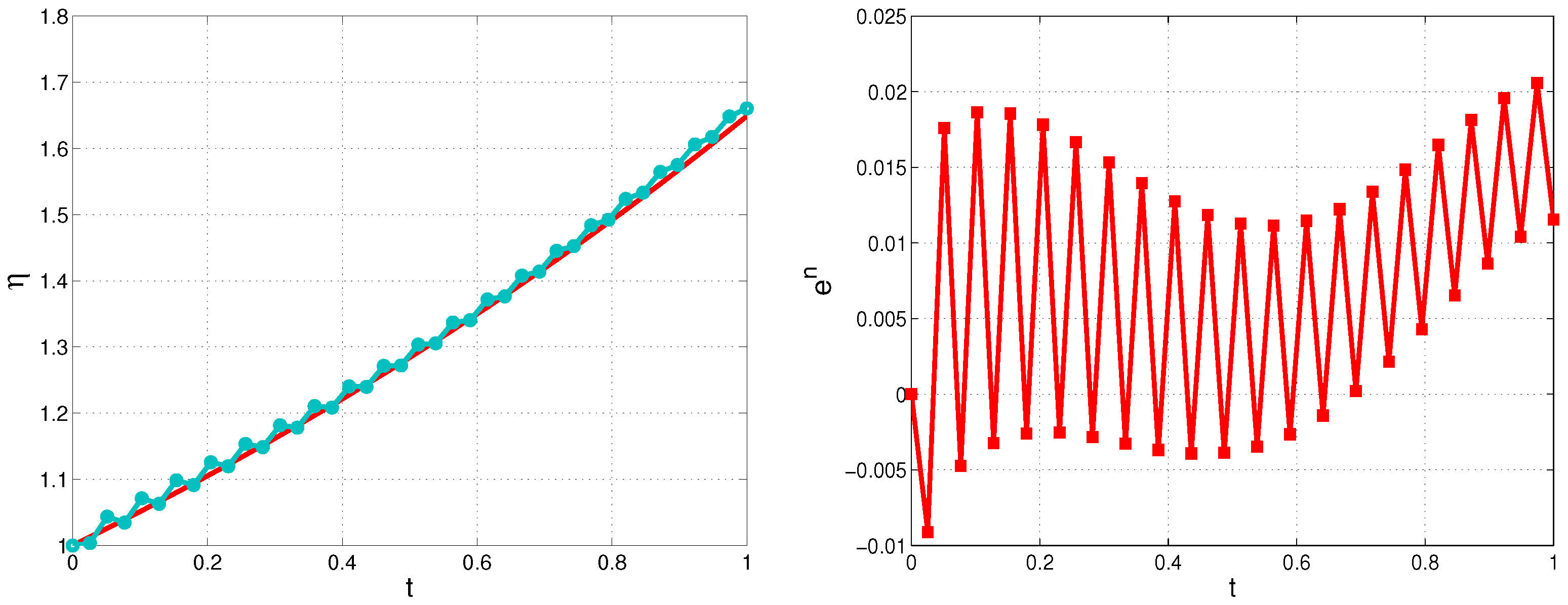
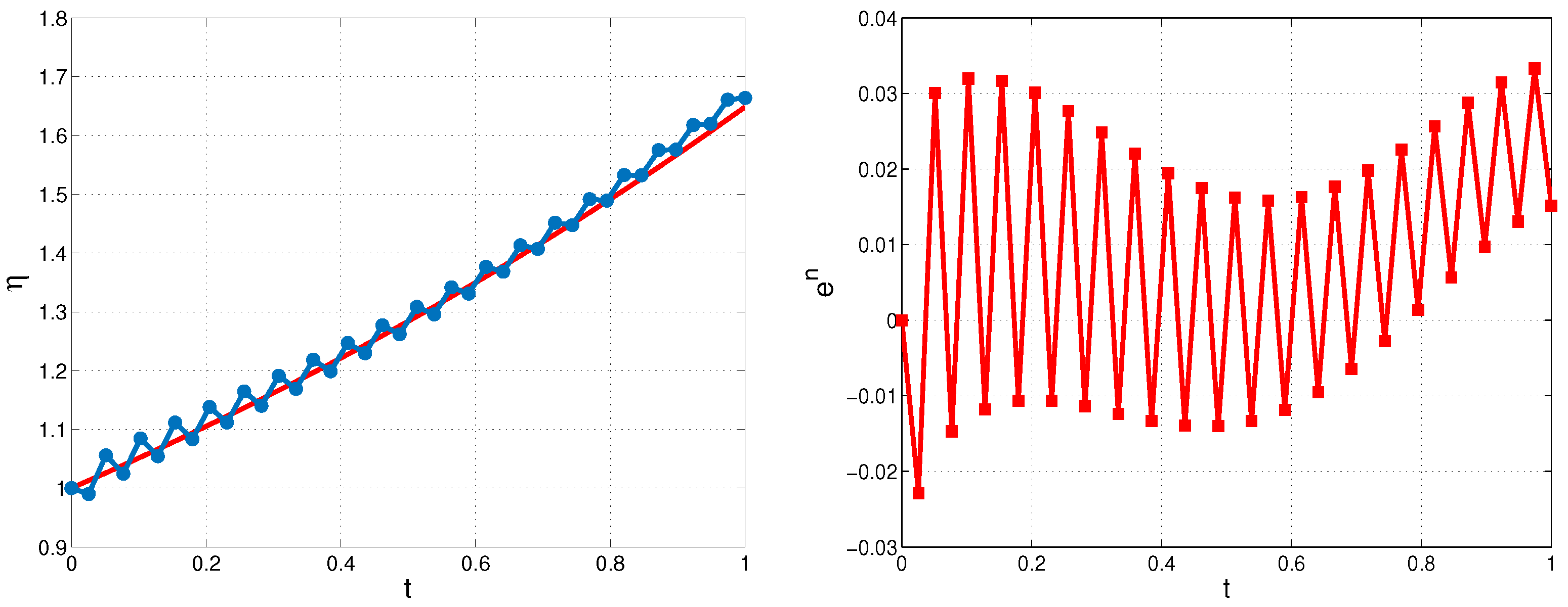
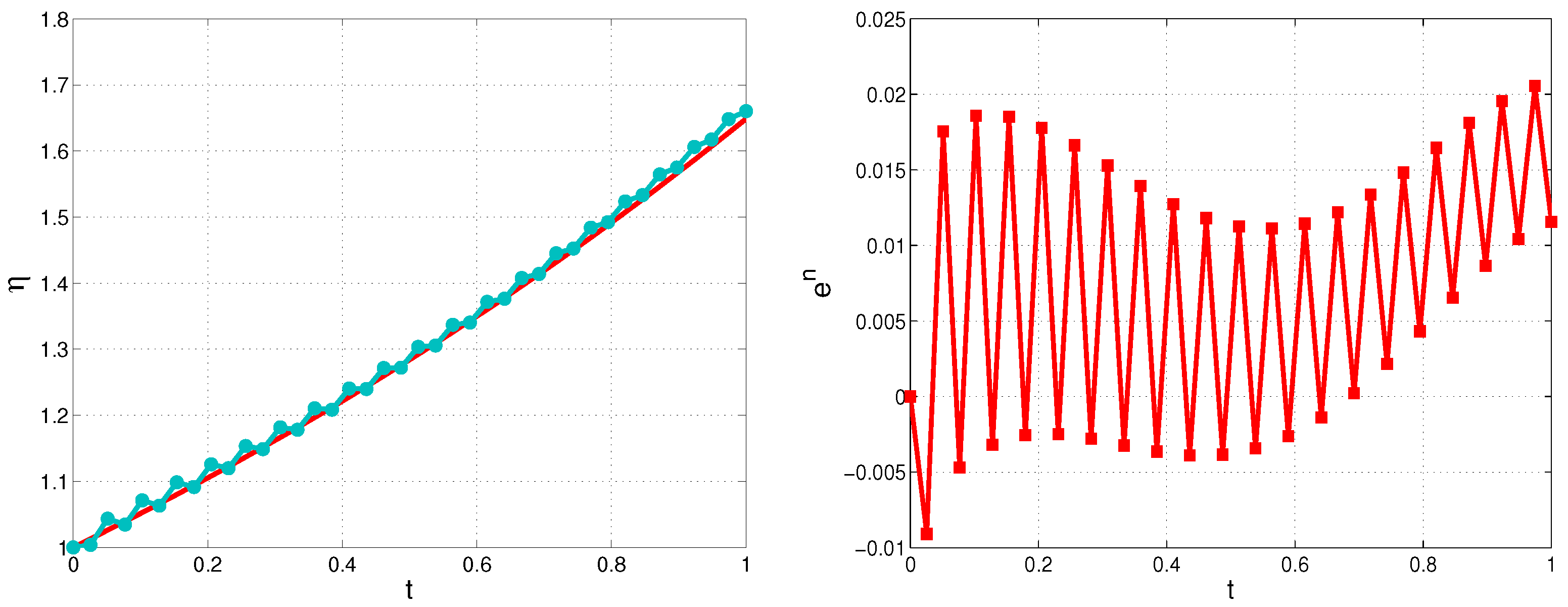
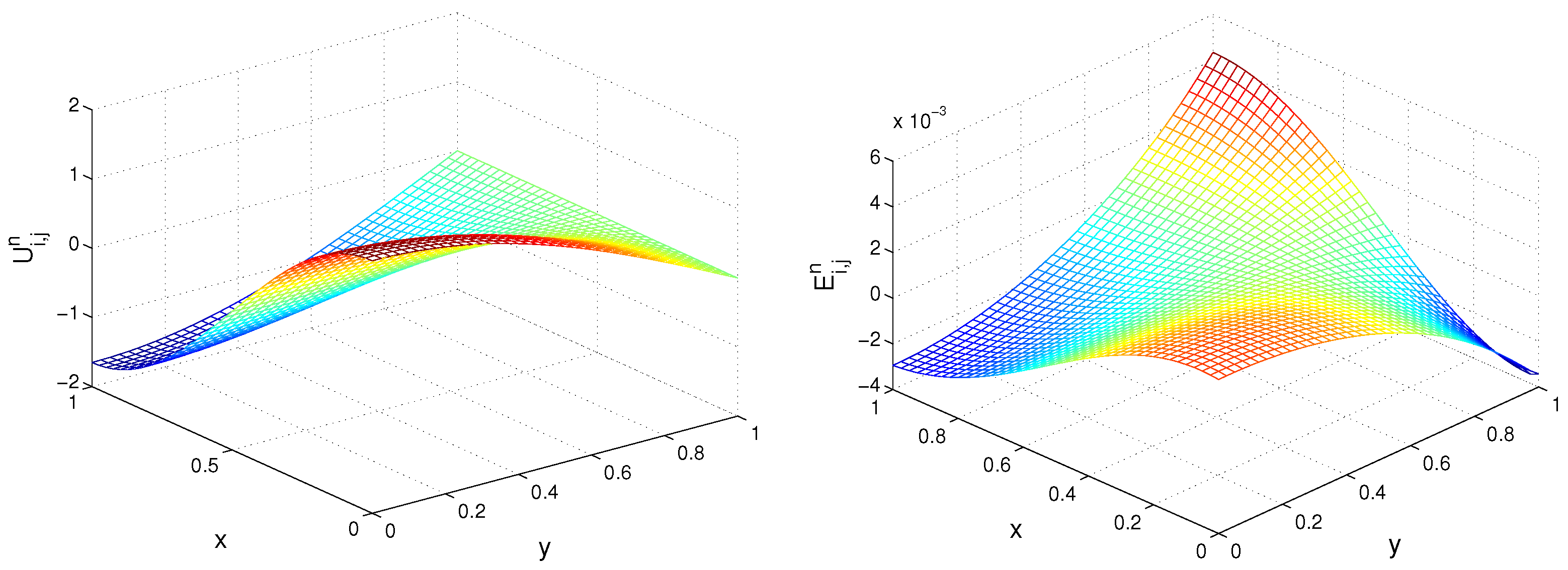
We consider the case $\tilde{\mu }=\mu$. In

Table 8. Errors of the solution of the inverse problem and recovered function $\eta \left(t\right)$ for different noise levels, PO, $x_p=0.5$, $\tilde{\mu }=\mu$, $\tau =h$, Example 3.

$\mathit{\rho }$	${\mathcal{E}}_{\mathit{\infty }}$	${\mathcal{E}}_2$	${\mathit{ϵ}}_{\mathit{\infty }}$	${\mathit{ϵ}}_2$
0.001	3.2432 $\times {10}^{-3}$	9.2110 $\times {10}^{-4}$	8.1036 $\times {10}^{-3}$	6.4731 $\times {10}^{-3}$
0.02	3.1853 $\times {10}^{-3}$	9.2206 $\times {10}^{-4}$	1.2942 $\times {10}^{-2}$	7.7720 $\times {10}^{-3}$
0.05	3.5603 $\times {10}^{-3}$	9.2568 $\times {10}^{-4}$	2.0581 $\times {10}^{-2}$	1.1616 $\times {10}^{-2}$
0.1	4.3447 $\times {10}^{-3}$	9.3730 $\times {10}^{-4}$	3.3313 $\times {10}^{-2}$	1.9557 $\times {10}^{-2}$

and

Table 9. Errors of the solution of the inverse problem and recovered function $\eta \left(t\right)$ for different noise levels, IO, $x_l=0.4$, $x_r=0.75$, $\tilde{\mu }=\mu$, $\tau =h$, Example 3.

$\mathit{\rho }$	${\mathcal{E}}_{\mathit{\infty }}$	${\mathcal{E}}_2$	${\mathit{ϵ}}_{\mathit{\infty }}$	${\mathit{ϵ}}_2$
0.001	3.2428 $\times {10}^{-3}$	9.2112 $\times {10}^{-4}$	8.1044 $\times {10}^{-3}$	6.4743 $\times {10}^{-3}$
0.02	3.1850 $\times {10}^{-3}$	9.2208 $\times {10}^{-4}$	1.2933 $\times {10}^{-2}$	7.7674 $\times {10}^{-3}$
0.05	3.5602 $\times {10}^{-3}$	9.2568 $\times {10}^{-4}$	2.0557 $\times {10}^{-2}$	1.1594 $\times {10}^{-2}$
0.1	4.3435 $\times {10}^{-3}$	9.3726 $\times {10}^{-4}$	3.3264 $\times {10}^{-2}$	1.9504 $\times {10}^{-2}$

we present errors of the solution of the inverse problem and recovered source $\eta \left(t\right)$ for different noise levels in the case of PO ($x_p=0.5$) and IO ($x_l=0.4$, $x_r=0.75$) for $\tau =h$, $I=40$. We observe that even for perturbed data, the numerical approach performs with good enough accuracy. In Figure 1 and Figure 2, we plot the exact recovered function η and the corresponding error for $\rho =0.05$ and $\rho =0.1$, while in Figure 3, we depict the exact numerical solution, obtained by solving the inverse problem and the corresponding error at the end of time in the case of PO ($x_p=0.5$), $\tau =h$, $I=40$. Similarly, in Figure 4, Figure 5 and Figure 6, we represent the results for IO ($x_l=0.4$, $x_r=0.75$) with the same mesh parameters.

For perturbed data, the boundary condition source is recovered with sufficient accuracy to ensure the optimal precision of the computed solution. This, we may deduce that the method is efficient for noisy measurements as well. This indicate the stability of the approach.

7. Conclusions

In this paper, we consider a pseudoparabolic equation on rectangular domain. We solve the inverse problem for unknown time-dependent boundary source on the base of point and integral observations on the same boundary. We establish the well-posedness of the direct problem. We also propose a new method to reduce the inverse problem to direct one. We developed a finite-difference method for solving both direct and inverse problems. The numerical results showed that the order of convergence of the finite-difference scheme for solving the direct problem is second order in space and first order in time. The same order of convergence has the numerical solution, recovered by inverse problem with exact measurements, both for point and integral observations. The determined time-dependent boundary source is of first order of convergence. In the case of noisy data, the boundary-source function and the solution are recovered by the numerical method with satisfactory precision. The method attains optimal accuracy for moderate levels of noise. It can be applied for different types of boundary conditions. Additionally, the method can be extended for boundary-condition inverse problems for semilinear pseudoparabolic equation [50].

In our future work, we plan to develop similar techniques for several classes of Sobolev-type equations of mathematical physics, such as Benjamin–Bona–Mahony equations, Boussinesque-type equations, etc. Also, similar inverse problems could be considered for nonlinear equations, for example those studied in [15].

References

1. Barenblat, G.I.; Entor, V.M.; Ryzhik, V.M. Theory of Fluid Flows Through Natural Rocks; Kluwer Academic Publishers: Dordrecht, The Netherlands, 1989. [Google Scholar]
2. Abreu, E.; Durán, A. Spectral discretizations analysis with time strong stability preserving properties for pseudo-parabolic models. Comput. Math. Appl. 2021, 102, 15–44. [Google Scholar] [CrossRef]
3. Pyatkov, S.G.; Shergin, S.N. On some mathematical models of filtration type. Bull. South Ural State Univ. Ser. Math. Model. Program. Comput. Softw. 2015, 8, 105–116. [Google Scholar]
4. Amar, M.; Andreucci, D.; Gianni, R.; Timofte, C. Well-posedness of two pseudo-parabolic problems for electrical conduction in heterogeneous media. J. Math. Anal. Appl. 2021, 493, 124533. [Google Scholar] [CrossRef]
5. Amirali, I.; Amiraliyev, G.M. Three layer difference method for linear pseudo-parabolic equation with delay. J. Comput. Appl. Math. 2022, 401, 113786. [Google Scholar] [CrossRef]
6. Amirali, I.; Amiraliyev, G.M. Numerical solution of linear pseudo-parabolic equation with time delay using three layer difference method. J. Comput. Appl. Math. 2024, 436, 115417. [Google Scholar] [CrossRef]
7. Barenblatt, G.I.; Bertsch, M.; Dal Passo, R.; Ughi, M. A degenerate pseudoparabolic regularization of a nonlinear forward-backward heat equation arising in the theory of heat and mass exchange in stably stratified turbulent shear flow. SIAM J. Math. Anal. 1993, 24, 1414–1439. [Google Scholar] [CrossRef]
8. Beshtokov, M.K. Boundary value problems for a pseudoparabolic equation with the Caputo fractional derivative. Differ. Equ. 2019, 55, 884–893. [Google Scholar] [CrossRef]
9. Düll, W.P. Some qualitative properties of solutions to a pseudoparabolic equation modeling solvent uptake in polymeric solids. Commun. Partial Differ. Equ. 2006, 31, 1117–1138. [Google Scholar] [CrossRef]
10. Manikandan, K.; Serikbayev, N.; Manigandan, M.; Sabareeshwaran, M. Dynamical evolutions of optical smooth positons in variable coefficient nonlinear Schrödinger equation with external potentials. Optik 2023, 288, 171203. [Google Scholar] [CrossRef]
11. Coleman, B.D.; Duffin, R.J.; Mizel, V.J. Instability, uniqueness, and nonexistence theorems for the equation ut = uxxuxtx on a strip. Arch. Ration. Mech. Anal. 1965, 19, 100–116. [Google Scholar] [CrossRef]
12. Showalter, R.E.; Ting, T.W. Pseudoparabolic partial differential equations. SIAM J. Math. Anal. 1970, 1, 1–26. [Google Scholar] [CrossRef]
13. Bouziani, A. Intial-boundary value problems for a class pseudoparabolic equations with integral boundary conditions. J. Math. Anal. 2004, 291, 366–371. [Google Scholar] [CrossRef]
14. Xie, M.; Tan, Z.; Wu, Z. Local existence and uniqueness of weak solutions to fractional pseudo-parabolic equation with singular potential. Appl. Math. Lett. 2021, 114, 106898. [Google Scholar] [CrossRef]
15. Kozhanov, A.I. Initial boundary value problem for generalized Boussinesque type equations with nonlinear source. Math. Notes 1999, 65, 59–63. [Google Scholar] [CrossRef]
16. Ngoc, L.T.P.; Uyen, K.T.T.; Nhan, N.H.; Longet, N.T. On a system of non-linear pseudoparabolic equations with Robin-Dirichlet boundary conditions. Commun. Pure Appl. Anal. 2022, 21, 585–623. [Google Scholar] [CrossRef]
17. Vromans, A.J.; van de Ven, F.; Muntean, A. Existence of weak solutions for a pseudo-parabolic system coupling chemical reactions, diffusion and momentum equations. arXiv 2017, arXiv:1702.02481. [Google Scholar]
18. Jachimaviciene, J.; Jeseviciute, Z.; Sapagovas, M. The stability of finite difference schemes for a pseudoparabolic equation with nonlocal conditions. Numer. Anal. Optim. 2009, 30, 988–1001. [Google Scholar] [CrossRef]
19. Wang, K. Two-grid methods for nonlinear pseudo-parabolic integro-differential equations by finite element method. Comput. Math. Appl. 2024, 168, 174–189. [Google Scholar] [CrossRef]
20. Sapagovas, M.; Štikonas, A.; Štikoniene, O. ADI method for pseudoparabolic equation with nonlocal boundary conditions. Mathematics 2023, 11, 1303. [Google Scholar] [CrossRef]
21. Woodbury, K.A.; Najafi, H.; de Monte, F.; Beck, J.V. Inverse Heat Conduction: Ill-Posed Problems, 2nd ed.; John Wiley & Sons, Inc.: Hoboken, NJ, USA, 2023. [Google Scholar]
22. Aitzhanov, S.; Isakhov, A.; Zhalgassova, K.; Ashurova, G. The coefficient inverse problem for a pseudoparabolic equation of the third order. J. Math. Mech. Comput. Sci. 2023, 119, 3–18. [Google Scholar] [CrossRef]
23. Burns, T.J.; Mates, S.P.; Rhorer, R.L.; Whitenton, E.P.; Basak, D. Inverse method for estimating shear stress in machining. J. Mech. Phys. Solids 2016, 86, 220–236. [Google Scholar] [CrossRef] [PubMed]
24. Lesnic, D. Inverse Problems with Applications in Science and Engineering; CRC Pres: Abingdon, UK, 2021; p. 349. [Google Scholar]
25. Hasanov, A.H.; Romanov, V.G. Introduction to Inverse Problems for Differential Equations, 1st ed.; Springer: Cham, Switzerland, 2017; 261p. [Google Scholar]
26. Isakov, V. Inverse Problems for Partial Differential Equations, 3rd ed.; Springer: Cham, Switzerland, 2017; p. 406. [Google Scholar]
27. Ivanov, V.K.; Vasin, V.V.; Tanana, V.P. Theory of Linear Ill-Posed Problems and Its Approximations; Nauka: Moscow, Russia, 1978. (In Russian) [Google Scholar]
28. Kabanikhin, S.I. Inverse and Ill-Posed Problems; DeGruyer: Berlin, Germany, 2011. [Google Scholar]
29. Prilepko, A.I.; Orlovsky, D.G.; Vasin, I.A. Methods for Solving Inverse Problems in Mathematical Physics; Marcel Dekker: New York, NY, USA, 2000. [Google Scholar]
30. Ruzhansky, M.; Serikbaev, D.; Torebek, B.T.; Tokmagambetov, N. Direct and inverse problems for time-fractional pseudo-parabolic equations. Quaest. Math. 2021, 45, 1071–1089. [Google Scholar] [CrossRef]
31. Huntul, M.J.; Khompysh, K.; Shazyndayeva, M.K.; Iqbal, M.K. An inverse source problem for a pseudoparabolic equation with memory. AIMS Math. 2024, 9, 14186–14212. [Google Scholar] [CrossRef]
32. Khompysh, K.; Huntul, M.J.; Shazyndayeva, M.K.; Iqbal, M.K. An inverse problem for pseudoparabolic equation: Existence, uniqueness, stability, and numerical analysis. Quaest. Math. 2024, 47, 1979–2001. [Google Scholar] [CrossRef]
33. Kozhanov, I. Inverse problems for determining boundary regimes for some equations of Sobolev type. Vestn. Yuzhno-Ural’skogo Univ. Seriya Mat. Model. Program. 2016, 9, 37–45. (In Russian) [Google Scholar] [CrossRef]
34. Lyubanova, A.S. An inverse problem for pseudoparabolic equationwith the mixed boundary condition. J. Sib. Fed. Univ. Math. Phys. 2023, 16, 661–672. [Google Scholar]
35. Lyubanova, A.S.; Tani, A. An inverse problem for pseudoparabolic equation of filtration: The existence, uniqueness and regularity. Appl. Anal. 2011, 90, 1557–1571. [Google Scholar] [CrossRef]
36. Lyubanova, A.S.; Tani, A. On inverse problems for pseudoparabolic and parabolic equations of filtration. Inverse Probl. Sci. Eng. 2011, 19, 1023–1042. [Google Scholar] [CrossRef]
37. Nikolaev, O.Y. Solvability of the linear inverse problem for the pseudoparabolic equation. Math. Notes NEFU 2023, 30, 58–66. [Google Scholar]
38. Baglan, I.; Kanca, F.; Mishra, V.N. Fourier method for an existence of quasilinear inverse pseudo-parabolic equation. Iran. J. Math. Sci. Inform. 2024, 19, 193–209. [Google Scholar] [CrossRef]
39. Fu, J.-L.; Liu, J. Recovery of a potential coefficient in a pseudoparabolic system from nonlocal observation. Appl. Numer. Math. 2023, 184, 121–136. [Google Scholar] [CrossRef]
40. Serikbaev, D. Inverse problem for fractional order pseudo-parabolic equation with involution. Ufimsk. Mat. Zh. 2020, 12, 122–138. [Google Scholar] [CrossRef]
41. Demir, A.; Ozbilge, E. Identification of the unknown boundary condition in a linear parabolic equation. J. Inequal. Appl. 2013, 2013, 96. [Google Scholar] [CrossRef]
42. Rundell, W.; Yin, H.-M. A parabolic inverse problem with an unknown boundary condition. J. Differ. Equ. 1990, 86, 234–242. [Google Scholar] [CrossRef]
43. Vasil’ev, V.I.; Su, L. Numerical method for solving boundary inverse problem for one-dimensional parabolic equation. Math. Model. 2017, 24, 108–117. [Google Scholar] [CrossRef]
44. Koleva, M.N.; Vulkov, L.G. Numerical reconstruction of time-dependent boundary conditions to 2D heat equation on disjoint rectangles at integral observations. Mathematics 2024, 12, 1499. [Google Scholar] [CrossRef]
45. Abdollahi, A.N.; Rostamy, D. Identifying an unknown time-dependent boundary source in time-fractional diffusion equation with a non-local boundary condition. J. Comput. Appl. Math. 2019, 355, 3–50. [Google Scholar]
46. Rundell, W.; Xub, X.; Zuo, L. The determination of an unknown boundary condition in a fractional diffusion equation. Appl. Anal. 2013, 92, 1511–1526. [Google Scholar] [CrossRef]
47. Koleva, M.N.; Vulkov, L.G. Numerical determination of a time-dependent boundary condition for a pseudoparabolic equation from integral observation. Computation 2024, 12, 243. [Google Scholar] [CrossRef]
48. Ladyzhanskya, A. Boundary Value Problems of Mathematical Physics, 1st ed.; Springer: New York, NY, USA, 1985. [Google Scholar]
49. Samarskii, A.A. The Theory of Difference Schemes; Marcel Dekker: New York, NY, USA, 2001. [Google Scholar]
50. Van Bockstal, K.; Khompysh, K. A time-dependent inverse source problem for a semilinear pseudo-parabolic equation with Neumann boundary condition. arXiv 2025, arXiv:2502.04821. [Google Scholar]
Figure 1. Exact (solid red line) and recovered (blue line with circles) boundary-source function  η  (left) and the corresponding error (right),  ρ = 0.05 τ = h μ ˜ = μ I = 40 , PO ( x p = 0.5 ), Example 3.
Mathematics 13 00908 g001
Figure 2. Exact (solid red line) and recovered (blue line with circles) boundary-source function  η  (left) and the corresponding error (left),  ρ = 0.1 τ = h μ ˜ = μ I = 40 , PO ( x p = 0.5 ), Example 3.
Mathematics 13 00908 g002
Figure 3. Exact and recovered solution (left) at the final time and the corresponding error (right),  ρ = 0.1 τ = h μ ˜ = μ I = 40 , PO ( x p = 0.5 ), Example 3.
Mathematics 13 00908 g003
Figure 4. Exact (solid red line) and recovered (blue line with circles) boundary-source function  η  (left) and the corresponding error (right),  ρ = 0.05 τ = h μ ˜ = μ I = 40 , PO ( x l = 0.4 x r = 0.75 ), Example 3.
Mathematics 13 00908 g004
Figure 5. Exact (solid red line) and recovered (blue line with circles) boundary-source function  η  (left) and the corresponding error (right),  ρ = 0.1 τ = h μ ˜ = μ I = 40 , PO ( x l = 0.4 x r = 0.75 ), Example 3.
Mathematics 13 00908 g005
Figure 6. Exact and recovered solution (left) at the final time and the corresponding error (right),  ρ = 0.1 τ = h μ ˜ = μ I = 40 , PO ( x l = 0.4 x r = 0.75 ), Example 3.
Mathematics 13 00908 g006