Evaluation Model for Indoor Comprehensive Environmental Comfort Based on the Utility Function Method

Abstract

Indoor environmental comfort is closely related to human health and well-being. This study aimed to establish a quantitative evaluation model for indoor comprehensive environmental comfort based on multiple physical environmental parameters. Firstly, based on the subjective evaluation characteristics of indoor environmental comfort and the principles of a multi-factor comprehensive evaluation, a comprehensive environmental comfort evaluation method utilizing the utility function approach was proposed. Secondly, subjective questionnaires and objective measurements were conducted in the indoor physical environment of rural dwellings in the Guanzhong Plain. The Kano model was employed to quantitatively analyze the influence of individual environmental comfort factors on the comprehensive environmental comfort based on the survey results. The findings revealed that thermal, lighting, and acoustic environments were the key influencing factors, while air quality was considered a non-key factor. Furthermore, quantitative relationships between environmental comfort and individual parameters were established, and the weights of individual environmental factors were determined using the analytic hierarchy process and the entropy weight method, based on the perspective of categorizing functional rooms and usage time periods. Finally, a quantitative evaluation model for indoor comprehensive environmental comfort was proposed that considered the one-vote veto characteristics and differentiated demands.

1. Introduction

In contemporary society, over 80% of our daily time is spent indoors, especially by vulnerable populations such as the elderly, infirm, ill, disabled, and pregnant individuals [1]. Therefore, having a well-maintained indoor environment is of critical importance. As indoor environmental comfort directly reflects the quality of the indoor environment, conducting research on the indoor environmental comfort evaluation becomes essential.

To date, scholars have conducted extensive research on indoor environmental comfort. Indraganti and Boussaa [2] evaluated the indoor thermal comfort of air-conditioned office buildings in Qatar and found that the comfortable indoor temperature was 24 ± 2.6 °C. Rajan et al. [3] surveyed the indoor thermal comfort of modern apartments in Japan and discovered that temperatures between 18 °C and 27.5 °C were comfortable for over 90% of the residents. Rijal [4] conducted a study on the thermal comfort of traditional houses in the Himalayan region of Nepal, revealing that due to long-term climate adaptation, the indoor neutral temperature of local dwellings was significantly lower, at only 9.7 °C. Fan et al. [5] conducted a study on indoor thermal comfort, focusing on rural dwellings in the Northwest region. Their results revealed that the comfortable indoor temperature varied depending on the functional room and usage time period. Specifically, the comfortable temperatures for the main and secondary functional rooms during activity periods were 15 °C and 12 °C, respectively, while the comfortable temperature for the main functional room during sleep periods was 13 °C. Mohd Husini et al. [6] found that the lower limit of comfortable illuminance for horizontal work surfaces in offices ranged between 300 lx and 500 lx. Zhu [7] indicated that 500 lx was the ideal illuminance, while 700 lx caused slight discomfort among office workers. Mui and Wong [8] conducted a subjective evaluation of acoustic comfort in office environments, indicating that the upper limit of comfortable noise level was 57.5 dB. Liu et al. [9] demonstrated through experimental research that noise levels exceeding 50 dB in open-plan offices could lead to physical discomfort. Iwashita et al. [10] assessed the indoor air quality comfort in Japanese courtrooms, revealing that when CO₂ concentration levels reached 1000 ppm, the dissatisfaction rate was approximately 20%. Li et al. [11] conducted research on indoor air quality in Hong Kong shopping centers and found that occupant satisfaction significantly decreased when the CO₂ concentrations exceeded 1000 ppm.

Furthermore, some scholars have conducted more in-depth research on comfort evaluation. For example, Djamila et al. [12] carried out on-site research on the thermal comfort conditions of residential areas in Kota Kinabalu, Malaysia. Based on the quantified relationship between thermal sensation votes and indoor air temperature, they proposed a thermal comfort evaluation model, indicating an indoor thermal neutral temperature of approximately 30 °C. Similarly, Yu et al. [13] conducted field research on indoor thermal comfort in rural buildings in the high-altitude regions of Tibet. Based on the survey results, they established an indoor thermal comfort evaluation model and determined the indoor neutral temperature. Guo [14] conducted an experimental study in an asymptomatic high-altitude area, demonstrating a quantitative relationship between illumination and comfort, thereby proposing an indoor lighting comfort evaluation model. Based on a synthesis of multiple research findings of indoor light comfort in Europe, Boer and de Fischer [15] established the quantitative relationship between indoor illuminance and the percentage of dissatisfaction. Additionally, Fanger [16] developed an indoor air quality comfort evaluation model based on the quantitative relationship between CO₂ concentration and the percentage of dissatisfaction. Clausen [17] established an indoor acoustic comfort evaluation model based on the quantitative relationship between noise levels and the percentage of dissatisfaction.

It is noteworthy that the aforementioned studies were often limited to individual environmental factors. In fact, indoor physical environments encompass multiple factors such as thermal, lighting, acoustic conditions, and air quality. Therefore, research on indoor physical environmental comfort should fully consider the combined effects of these individual factors. Using comprehensive comfort under the influence of multiple environmental factors as an evaluation indicator can more reasonably and accurately reflect indoor comfort conditions.

In recent years, some scholars have conducted research on comprehensive indoor environmental comfort evaluation based on multiple environmental factors. Based on field measurements and questionnaire surveys, Li et al. [18] conducted a study on the comfort of open-plan offices in severe cold regions. They revealed the quantified relationship between environmental comfort and indoor environmental parameters, determined the weighting coefficients of each evaluation factor, and subsequently proposed an evaluation model for indoor comprehensive environmental comfort using multiple linear regression. Similarly, Guo et al. [19] conducted experimental research in an environmental simulation chamber, clarified the quantitative relationship between individual environmental parameters and environmental comfort, as well as the weights of individual environmental factors. Subsequently, they established a quantitative evaluation model for comprehensive human comfort using the penalty substitution synthesis model. In addition, Fassi et al. [20], Catalina and Iordache [21], and Yang and Mark [22] conducted surveys on classrooms; Li [23], as well as Ncube and Riffat [24] carried out research on offices; and Lai et al. [25] investigated high-rise residential buildings. They all adopted evaluation methods similar to those mentioned above and each has developed a comprehensive indoor environmental evaluation model. These research findings provide a theoretical basis for the evaluation and improvement of indoor environmental comfort.

However, research on the quantitative evaluation of comprehensive indoor environmental comfort has mainly focused on office and educational buildings, while studies on residential buildings, particularly rural dwellings, have been scarcely reported. A variety of evaluation methods exist for comprehensive environmental comfort, but a consensus has not yet been reached.

Previous studies emphasized that individual environmental comfort held a veto power over comprehensive environmental comfort; however, the existing evaluation models often fail to reflect this critical characteristic. Additionally, although several studies demonstrated that the residents had differentiated demands for indoor physical environment in terms of functional rooms and usage time periods, research on residential buildings did not take this characteristic into account. Consequently, the existing theoretical framework for comprehensive indoor environmental comfort evaluation remained incomplete and necessitates further refinement and expansion.

The Guanzhong Plain, a crucial cradle of Chinese civilization, is located in the core region of China’s inland hinterland. The local rural areas are characterized by a large population and a substantial number of buildings. However, constrained by factors such as climate conditions, economic levels, and scientific theories, there are prominent issues regarding unsatisfactory indoor physical environments and low indoor environmental comfort [26,27]. Therefore, it is particularly necessary and urgent to conduct research on the evaluation of indoor physical environmental comfort in rural dwellings in the Guanzhong Plain. The aim is to provide a theoretical basis for the scientific evaluation and creation of comfortable and livable rural living environments in the Guanzhong Plain and similar areas.

2. Methods

2.1. Field Survey

2.1.1. Survey Location

The Guanzhong Plain, located in the central part of Shaanxi Province, is situated in the core area of China’s inland hinterland. The area experiences cold winters and hot summers, with a relatively fragile ecological environment and a comparatively lagging economic development. From 2020 to 2024, our research team conducted field investigations on the rural dwellings in this area, during January and July, each year. This study covered 49 villages across five administrative regions in the Guanzhong Plain. The selected villages were representative in terms of living habits, architectural characteristics, and economic levels, and could well reflect the indoor environment status of rural dwellings in the Guanzhong Plain.

2.1.2. Subjective Questionnaire

This study strictly adhered to the ethical guidelines outlined in the Declaration of Helsinki and was approved by the Human Research Ethics Committee of Xi’an University of Technology (No. XAUT-EC20191202). Prior to the commencement of the survey, all participants provided written informed consent after fully understanding relevant information such as the research objectives, data usage, and privacy protection clauses. All respondents were local rural residents, but individuals were excluded if they were likely unable to accurately complete the questionnaire due to health, age, or cognitive reasons. During the survey period, participants maintained their normal daily activities, including diet, sleep, and habits. The basic information of the participants is presented in

Table 1. The basic information of the respondents.

Classification	Background	Percentage (%)
Gender	Male	47.1
	Female	52.9
Age	18~35	14.2
	36~55	29.5
	56~75	56.3
Educational level	Junior high school or lower	57.8
	High school	32.2
	Associate degree	7.1
	Bachelor’s degree or higher	2.9

. In the collection of survey results, questionnaires with a completion rate of less than 90% and abnormal objective monitoring data were excluded.

According to the survey, the thermal resistance of residents’ winter clothing was concentrated in the range of 1.55 clo to 2.05 clo during active periods, and in the range of 0.40 clo to 0.75 clo during sleep periods. For summer clothing, the thermal resistance was concentrated in the range of 0.45 clo to 0.85 clo during active periods, and in the range of 0.30 clo to 0.55 clo during sleeping periods. Given the sedentary state of the participants, their metabolic rate was approximately 1.1 met [28]. During sleep periods in the winter, residents generally preferred using heated thick bedding with temperatures ranging from 30 °C to 38 °C to adapt to the relatively cold indoor environment. During the summer sleep period, residents commonly adjusted the coverage of blankets or thin quilts dynamically based on their thermal sensations to effectively enhance thermal comfort.

In the survey, the comfort votes used a five-point scale: comfortable (0), slightly uncomfortable (−1), uncomfortable (−2), significantly uncomfortable (−3), and very uncomfortable (−4).

2.1.3. Objective Measurements

During the administration of the subjective questionnaire in households, indoor environmental parameters were also measured. The specific parameters measured are listed in

Table 2. Measurement parameters and corresponding instruments.

Measurement Parameters	Measurement Instruments	Type	Range	Accuracy
Temperature	Temperature and humidity recorder	SW-572	−20~60 °C	±0.3 °C
Noise level	Sound level meter	AWA6291	25~140 dB(A)	±1%
CO2 concentration	CO2 detector	SW-723	0~9999 ppm	±(40 + 3%) ppm
Illuminance	Illuminance meter	JTG01	0.1~100,000 lx	±4%

. All instruments were calibrated prior to use. During the measurement process, the instruments were placed in the immediate vicinity of the respondents. The measurement point for indoor natural lighting illuminance was located 0.75 m above the floor, while the measurement points for other parameters were situated 1.2 m above the floor.

2.2. Indoor Comprehensive Environmental Comfort Evaluation Method

2.2.1. Multi-Factor Comprehensive Evaluation Method

Multi-factor comprehensive evaluation is a commonly used decision analysis method, primarily employed to comprehensively consider multiple related factors or indicators to assess their overall performance [29]. The indoor physical environment is influenced by various environmental factors, which makes the evaluation of indoor comprehensive environmental comfort a typical multi-index comprehensive evaluation problem.

Commonly used multi-factor comprehensive evaluation methods include fuzzy comprehensive evaluation method [30,31], utility function comprehensive evaluation method [19,32], multivariate statistical comprehensive evaluation method [33,34], gray system comprehensive evaluation method [7,35], and artificial neural network comprehensive evaluation method [36,37].

Among these, the utility function comprehensive evaluation method shares many similarities in form with the aforementioned methods. Moreover, its uniqueness lies in its relatively simple calculation process, making the evaluation results more intuitive and easier to understand. Therefore, this study adopted the comprehensive evaluation method based on the utility function method, as expressed in [19]:

$$F=\xi \left(y_i;{\omega }_i\right),y_i=f_i\left(x_i\right)$$

(1)

where F is the comprehensive evaluation value, x_i represents the evaluation indicator, f_i is the utility function of x_i, y_i is the utility function evaluation value of x_i, ω_i is the weight of x_i, and ξ is the composite model.

According to Equation (1), the core of the utility function comprehensive evaluation method lies in the establishment of the utility function f_i, the calculation of the weights ω_i, and the determination of the synthesis model ξ.

2.2.2. Principles for Determining Utility Function

In fact, not all functions y = f (x) can serve as utility functions. For a function to qualify as a utility function, it needs to meet the following requirements:

(1)

y is related to x and only to x;

(2)

y is independent of the measurement units of x;

(3)

y = f (x) has a relatively clear range of values or critical points;

(4)

The results of y = f (x) are intuitive and have clear physical meanings;

(5)

Within the same indicator system, for different x values, different forms of y = f (x) may be used;

(6)

The range of values for y = f (x) should meet the requirements of the composite model;

(7)

The type and form of y = f (x) should be selected based on the impact of changes in x on the evaluation object;

(8)

Under the premise that the direction, concavity, and other characteristics of y = f (x) are clear, its form should be simplified as much as possible.

2.2.3. Weight Calculation Method

The commonly used methods for weight calculation can be categorized into three types: subjective, objective, and combined weighting methods. Among these, the combined weighting method can balance the negative impact of subjective and objective evaluation methods on the comprehensive evaluation results. Therefore, this study adopted the combined weighting method to calculate the final weights. Specifically, a linear weighted combination of the Analytic Hierarchy Process (AHP) and entropy weight method (EWM) was used to determine the weights.

a.

Weight calculation using AHP [38]

(1)

Matrix construction. Based on the evaluations of the experts for each indicator, the importance of pairwise indicators is compared using a 1–9 scale [39] to construct an n × n judgment matrix A.

$$\mathit{A}={\left(a_{ij}\right)}_{m\times n}={\left[\begin{array}{llll}{a}_{11}& a_{12}& \cdots & a_{1n}\\ a_{21}& a_{22}& \cdots & \cdots \\ \cdots & \cdots & \cdots & \cdots \\ a_{m1}& a_{m2}& \cdots & a_{nn}\end{array}\right]}_{m\times n}$$

(2)

where a_ij (i, j = 1, 2, 3, … n) is the relative importance of pairwise indicator comparisons, $a_{ij}=1/a_{ji}$, $a_{ii}=1$.

(2)

Calculate weights.

First, compute the sum of each column in the judgment matrix A:

$$S_j={\displaystyle \sum _{i=1}^n{a}_{ij}}$$

(3)

Next, each element in the matrix is divided by the sum of its corresponding column to obtain the normalized matrix $\mathit{B}$:

$$b_{ij}={\displaystyle \frac{a_{ij}}{S_j}}$$

(4)

Then, calculate the average of each row in the normalized matrix B to obtain the weight vector $\mathit{\omega }$:

$${\omega }_i={\displaystyle \frac{1}{n}}{\displaystyle \sum _{j=1}^n{b}_{ij}}$$

(5)

(3)

Consistency test.

$$CI={\displaystyle \frac{{\lambda }_{\max }-n}{n-1}}$$

(6)

$$CR={\displaystyle \frac{CI}{RI}}$$

(7)

where CI is the consistency indicator, RI is the average random consistency indicator, and CR is the consistency ratio (if CR is less than 0.1, it is considered that the judgment matrix A has passed the consistency).

(4)

Weight determination. The eigenvectors corresponding to the maximum eigenvalues are normalized to obtain the weights of each evaluation indicator.

b.

Weight calculation using EWM [40]

(1)

Matrix construction. Assuming that there are m samples and n indicators, an n × m evaluation matrix A is constructed based on the expert scores for each indicator.

$$\mathit{A}={\left(a_{ij}\right)}_{m\times n}={\left[\begin{array}{llll}{a}_{11}& a_{12}& \cdots & a_{1n}\\ a_{21}& a_{22}& \cdots & \cdots \\ \cdots & \cdots & \cdots & \cdots \\ a_{m1}& a_{m2}& \cdots & a_{mn}\end{array}\right]}_{m\times n}$$

(8)

where $a_{ij}$ (i = 1, 2, 3,…, m; j = 1, 2, 3,…, n) represents the original scores of the i^-th evaluation object on the j^-th evaluation criterion.

The scores were determined through expert voting, with voting options categorized as “very important”, “relatively important”, “average”, “not very important”, and “unimportant”, corresponding to grade scores of 5, 4, 3, 2, and 1 points, respectively.

The calculation expression for the voting scores is as follows:

$$R={\displaystyle \sum _{i=1}^m{X}_i}{V}_i$$

(9)

where R represents the indicator score, V_i is the score of the i^-th evaluation level for the indicator, X_i is the proportion of votes for the i^-th evaluation level of the indicator, and n represents the number of evaluation levels.

(2)

Data standardization. Different evaluation indicators have distinct dimensions and units. To eliminate the influence of differing dimensions and units on evaluation results, data standardization is necessary. The standardization method is as follows:

$$\begin{array}{l}{r}_{ij}={\displaystyle \frac{a_{ij}-\min (a_j)}{\max (a_j)-\min (a_j)}}\left(\mathrm{positive} \mathrm{indicators}\right)\\ r_{ij}={\displaystyle \frac{\max (a_j)-a_{ij}}{\min (a_j)-min(a_j)}}\left(\mathrm{negative} \mathrm{indicators}\right)\end{array}$$

(10)

where r_ij represents the standardized value of the j^-th indicator for the i^-th sample.

(3)

Entropy value calculation.

$$\begin{array}{l}{e}_j=-{\displaystyle \frac{1}{\mathrm{In}m}}{\displaystyle \sum _{i=1}^m{p}_{ij}\mathrm{In}}{p}_{ij}\\ p_{ij}={\displaystyle \frac{r_{ij}}{{\displaystyle {\sum }_{i=1}^m{r}_{ij}}}}\end{array}$$

(11)

where e_j is the entropy value of the j^-th indicator, and p_ij is the proportion of the i^-th sample under the j^-th indicator.

(4)

Entropy weight determination.

$$\begin{array}{l}{\omega }_j={\displaystyle \frac{d_j}{{\displaystyle \sum _{i=1}^m{d}_j}}}\\ d_j=1-e_j\end{array}$$

(12)

where ω_j is the weight of the j^-th indicator, and d_j is the differentiation coefficient of the j^-th indicator.

c.

Combined weight calculation [41]

The combined weight of the evaluation indicators is calculated based on the linear weighted synthesis method.

$${\omega }_{cj}=a\cdot {{\omega }_j}^{\mathrm{AHP}}+b\cdot {{\omega }_j}^{\mathrm{EWM}}$$

(13)

where ω_cj is the combined weight of the j^-th indicator; ω_j^AHP and ω_j^EWM are the subjective weight and objective weight of the j^-th indicator, respectively; and a and b are the proportional coefficients for the subjective weight and objective weight, respectively.

An optimization function was established with the objective of minimizing the sum of squared errors between the combined weights and the subjective weights, as well as between the combined weights and the objective weights. The specific formula is as follows:

$$\left\{\begin{array}{l}\underset{a,b}{\min }={\displaystyle \sum _{j=1}^m\left[{\left({\omega }_{cj}-{{\omega }_j}^{\mathrm{AHP}}\right)}^2+{\left({\omega }_{cj}-{{\omega }_j}^{\mathrm{EWM}}\right)}^2\right]}\\ a+b=1, a>0, b>0 \end{array}\right.$$

(14)

When α is equal to 0.5, the sum of squared errors is minimized. Thus, the formula for calculating the combined weights was as follows:

$${\omega }_{cj}=0.5{{\omega }_j}^{\mathrm{AHP}}+0.5{{\omega }_j}^{\mathrm{EWM}}$$

(15)

2.2.4. Model Synthesis Method

Currently, synthesis models are mainly classified into two categories: power mean synthesis models (such as arithmetic mean, harmonic mean, quadratic mean, and geometric mean synthesis models) and special synthesis models (such as mixed, substitution, and piecewise synthesis models).

The evaluation concepts of these composite models vary, so the correct choice should be made based on research needs. However, it is important to emphasize that the penalty substitution synthesis model embodies a penalty principle, where the comprehensive evaluation result will be the worst if any single evaluation indicator performs the worst, reflecting the characteristic of a one-vote veto. Furthermore, this model also reflects a synergistic evaluation principle, meaning that individual evaluation indicators do not act independently but rather interact synergistically to influence the final comprehensive evaluation result. These two evaluation concepts coincide with the selection criteria of this paper. Therefore, the penalty substitution synthesis model was adopted in establishing the evaluation model for indoor environmental comprehensive comfort. The expression for the penalty substitution synthesis model is as follows [19]:

$$F=L+{{\displaystyle \prod _{i=1}^n\left(y_i-L\right)}}^{{\omega }_i}$$

(16)

where F is the comprehensive evaluation value, L is the theoretical minimum value of the evaluation indicator, y_i is the utility function of the evaluation indicator x_i, and ω_j is the weight of the evaluation indicator x_i.

2.3. Key Environmental Factors Analysis Method

2.3.1. Multi-Factor Analysis Method

In a multi-factor analysis, methods such as the Analytic Hierarchy Process (AHP), Structural Equation Modeling (SEM), and the Kano Model (KM) have been widely applied. Notably, the KM is capable of capturing the nonlinear relationship between environmental factors and subjective perceptions, whereas AHP is based on linear additive assumptions, making it more suitable for addressing weight allocation among explicit variables. Although SEM can handle relationships among multiple variables, it demands high-quality data and involves a relatively complex analysis process. In addition, compared to AHP and SEM, the KM places a greater emphasis on user emotions and preferences, as well as the systematic classification and prioritization of influencing factors, thereby providing decision-makers with a more explicit and effective basis. Additionally, the KM has been extensively applied in the field of comprehensive environmental comfort research. Kim and de Dear [42] were the first to apply the KM to research on indoor architectural environments. Using the database from the Center for the Built Environment (CBE), they validated the applicability of the KM, analyzed the correlation between individual environmental satisfaction and comprehensive environmental satisfaction, and identified various key environmental factors. Later, Zhang [43] and Geng et al. [44] conducted field surveys on high-speed rail stations and airport terminals, respectively. On the basis of revealing the mechanisms by which individual environmental comfort factors influence overall environmental comfort, they identified the key environmental factors. In summary, the KM was considered to be a reasonable and applicable analytical tool in exploring key environmental factors that affect comprehensive environmental comfort. Given that the applicability of this model has been verified in previous research, this paper directly applied the KM in analyzing key environmental factors.

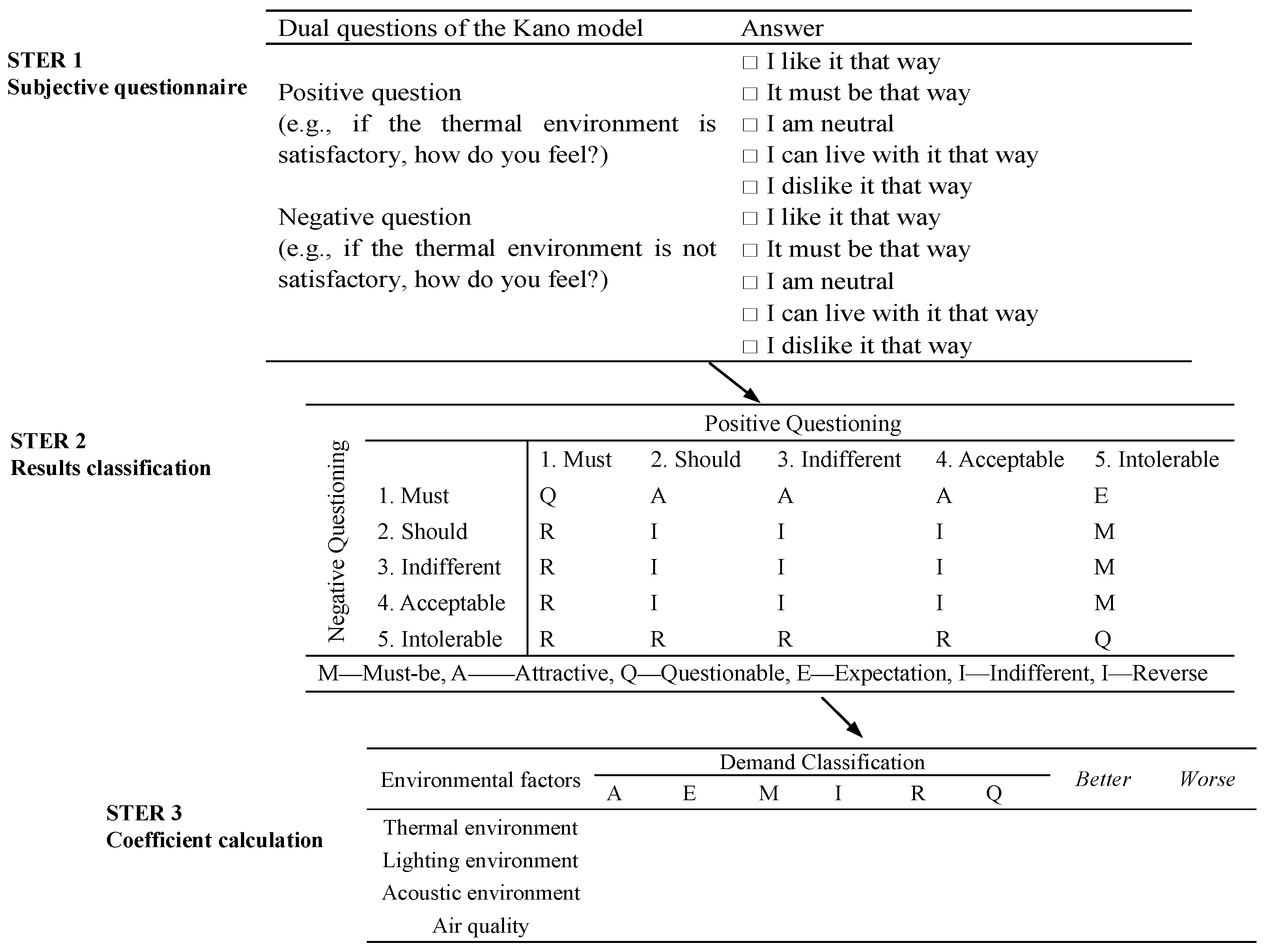
2.3.2. Overview of the Kano Model

In the 1980s, Professor Noriaki Kano of the Tokyo Institute of Technology developed the KM [45]. This model categorizes user demands into five distinct types: must-be, expectation, attractive, indifferent, and reverse. The factors corresponding to these five demand attributes are as follows: must-be factors, expectation factors, attractive factors, indifferent factors, and reverse factors.

Must-be factors: poor performance significantly reduces comprehensive comfort, while exceptional performance results in only limited improvement.

Expectation factors: excellent performance significantly enhances comprehensive comfort, while poor performance significantly reduces it.

Attractive factors: As performance improves, comprehensive comfort increases accordingly. However, once needs are met, even average performance maintains a high comfort level. Conversely, the comprehensive comfort level does not decrease significantly even if needs remain unmet.

Indifferent factors: regardless of performance, there is no impact on comprehensive comfort.

Reverse factors: excellent performance decreases comprehensive comfort.

Since indifferent and reverse factors do not positively enhance comprehensive comfort, this paper does not focus on them.

The main steps of the KM calculation include questionnaire survey, results classification, and coefficient calculation (see Figure 1). The formulas for calculating the Better and the Worse coefficients are as follows [46]:

$$Better={\displaystyle \frac{A+E}{A+E+M+I}}$$

(17)

$$Worse=-{\displaystyle \frac{E+M}{A+E+M+I}}$$

(18)

where Better represents the comfort coefficient, which is positive value. The closer the value is to 1, the greater the improvement in comfort. Worse stands for the discomfort coefficient, which is negative value. The closer the value is to −1, the greater the reduction in comfort.

After completing the above steps, a four-quadrant diagram was created based on Better and |Worse| values to classify and prioritize each environmental factor. The characteristics of each quadrant of the four-quadrant diagram are as follows:

First quadrant: high values for both Better and |Worse|. Factors in this quadrant are referred to as “Expectation Factors”.

Second quadrant: high Better value but low |Worse| value. Factors in this quadrant are known as “Attractive Factors”.

Third quadrant: low values for both Better and |Worse|. Factors in this quadrant are termed “Indifferent Factors”.

Fourth quadrant: low Better value but high |Worse| value. Factors in this quadrant are classified as “Must-be Factors”.

3. Results and Analysis

3.1. Key Environmental Factors

Based on the results of the Kano questionnaire, the environmental factors were classified into different attributes. Based on this, the Better coefficient and the Worse coefficient were calculated according to Equations (17) and (18). The aforementioned results are presented in

Table 3. Results of the Kano model.

Environmental Factors	Demand Classification						Better	Worse
	A	E	M	I	R	Q
Thermal environment	368	332	86	3	0	5	0.53	−0.89
Lighting environment	322	327	135	4	0	6	0.58	−0.83
Acoustic environment	339	327	115	4	0	9	0.56	−0.85
Air quality	210	320	199	58	0	7	0.66	−0.67

.

A Better–|Worse| four-quadrant diagram was constructed using the average Better and |Worse| values as the coordinate center, with |Worse| as the horizontal axis and Better as the vertical axis (see Figure 2). It can be observed that the thermal environment, lighting environment, and acoustic environment were all categorized as must factors, while indoor air quality was classified as an attractive factor. Poor performance in must factors had a significant negative impact on comprehensive comfort, whereas poor performance in attractive factors had almost no negative impact. Therefore, this paper identified the thermal environment, light environment, and acoustic environment as the key factors influencing indoor overall comfort, and considered air quality as a non-key factor. Based on this, the subsequent analysis focused solely on the three key factors: thermal, lighting, and acoustic environments.

3.2. Individual Environmental Comfort

A questionnaire survey was conducted to assess indoor temperature, illuminance, and acoustic comfort levels, based on a research perspective distinguishing functional rooms and usage time periods. Subsequently, the residents’ subjective voting results were further analyzed. Based on the comfort evaluation scale, a value of −1 (slightly uncomfortable) was set as the lower threshold, defining the range between −1 and 0 as the comfort voting interval.

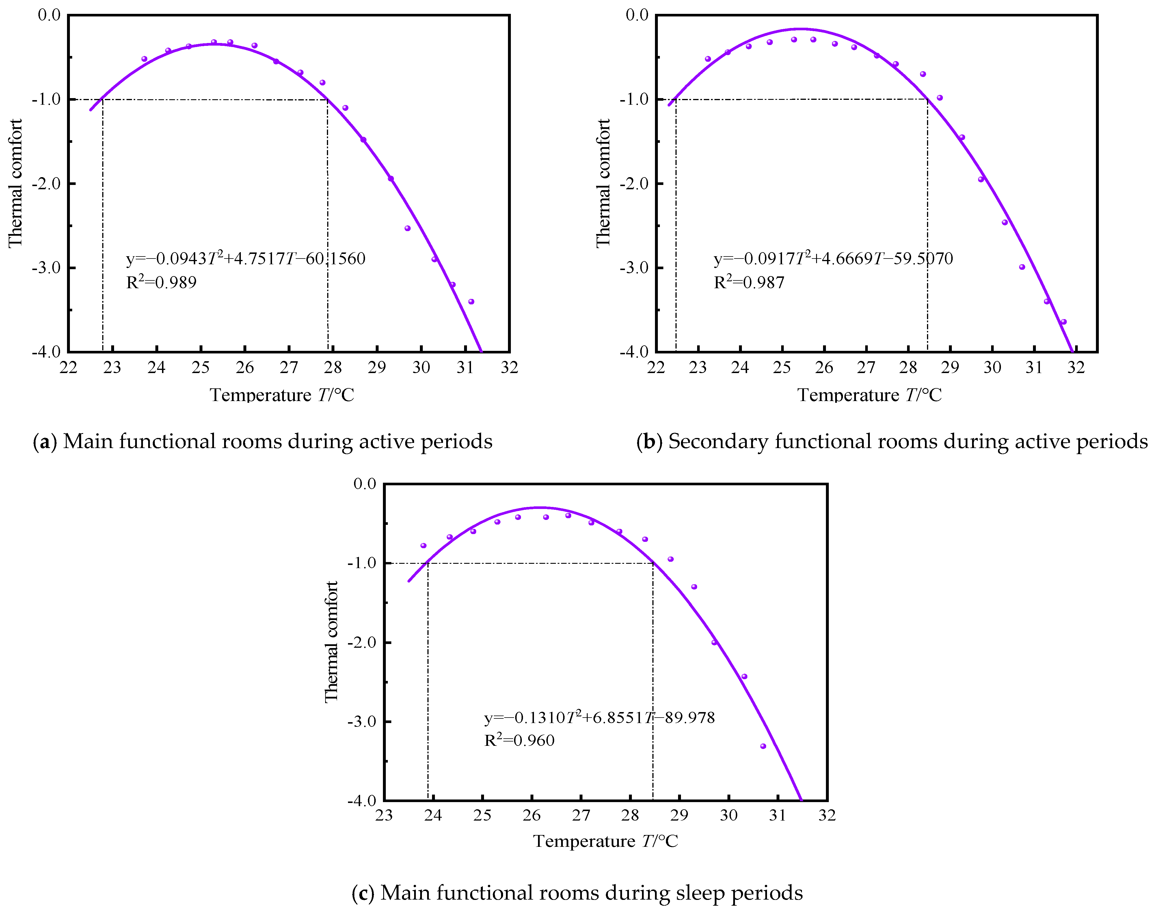
3.2.1. Thermal Environment

The quantitative relationship between temperature and thermal comfort was established by fitting the data, using the average value of each temperature interval as the independent variable and the average value of thermal comfort voting results as the dependent variable (see Figure 3 and Figure 4). The results showed that the thermal comfort vote values followed a nonlinear trend, first increasing and then decreasing as the indoor temperature rose. According to the fitting results, the comfortable temperature range for secondary functional rooms during active periods was broader than that for main functional rooms. For main functional rooms, the comfortable temperature range during sleep periods was broader than that during active periods.

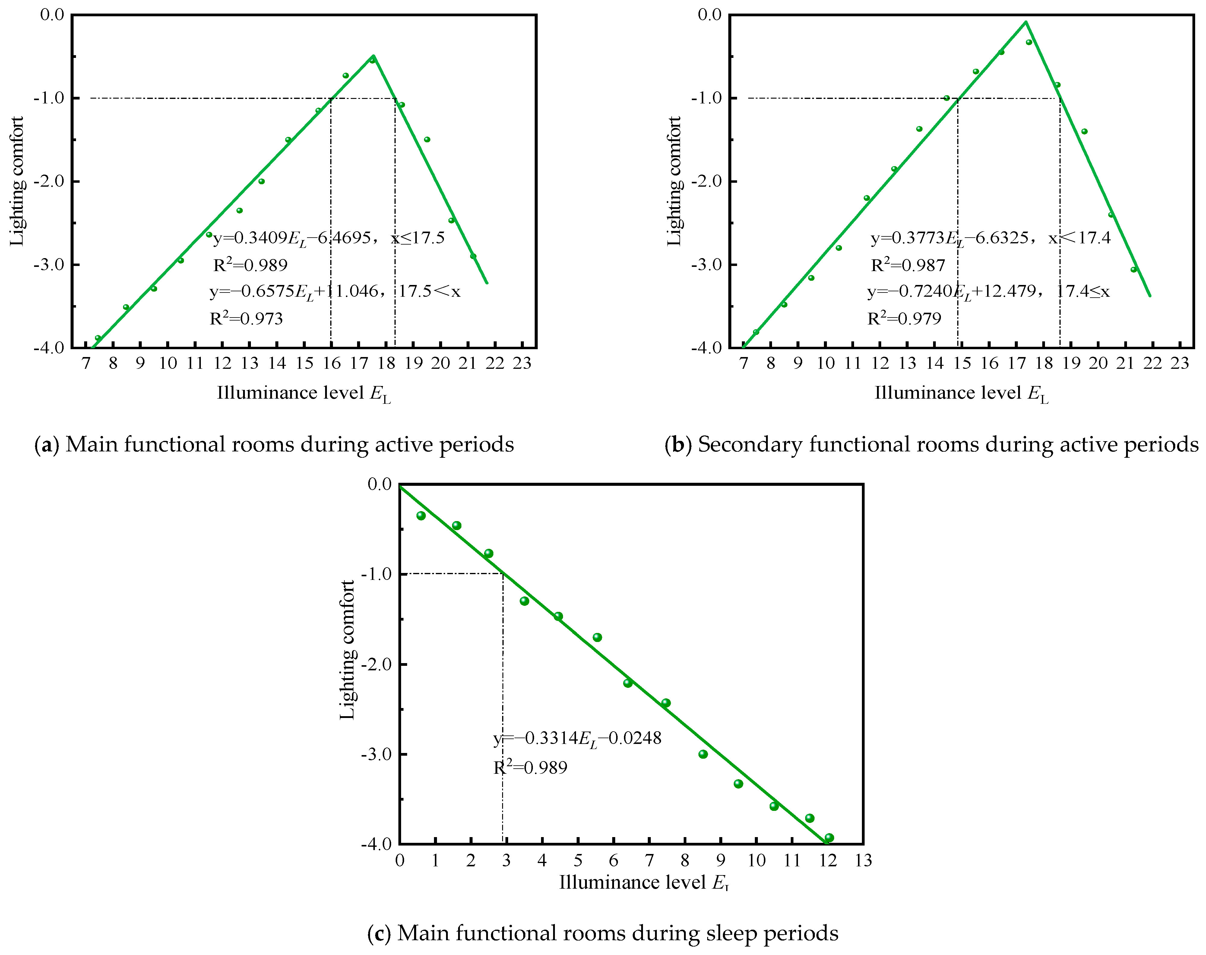
3.2.2. Luminous Environment

With reference to the standards [47] and field surveys, the indoor illuminance standard values were classified, and the corresponding relationship between illuminance levels and illuminance values was established, as detailed in

Table 4. The correspondence between illuminance and illuminance level.

Illuminance Value	Illuminance Level	Illuminance Value	Illuminance Level
0~0.25	0~1	75~100	12~13
0.25~0.5	1~2	100~150	13~14
0.5~1	2~3	150~200	14~15
1~2	3~4	200~300	15~16
2~3	4~5	300~500	16~17
3~5	5~6	500~750	17~18
5~10	6~7	750~1000	18~19
10~15	7~8	1000~1500	19~20
15~20	8~9	1500~2000	20~21
20~30	9~10	2000~3000	21~22
30~50	10~11	3000~5000	22~23
50~75	11~12	——	——

.

The quantified relationship between indoor illuminance levels and visual comfort was established by fitting the data, using the average value of each illuminance level interval as the independent variable and the average value of visual comfort voting results as the dependent variable (see Figure 5). During active periods, the lighting comfort vote values showed a trend of monotonically increasing, followed by monotonically decreasing, with an increase in indoor illuminance levels, while during sleep periods, a monotonically decreasing trend was observed. According to the fitting results, it was found that the comfortable illuminance range for secondary functional rooms was broader than that for main functional rooms during active periods. For main functional rooms, the difference in comfortable illuminance ranges between active and sleep periods was highly significant.

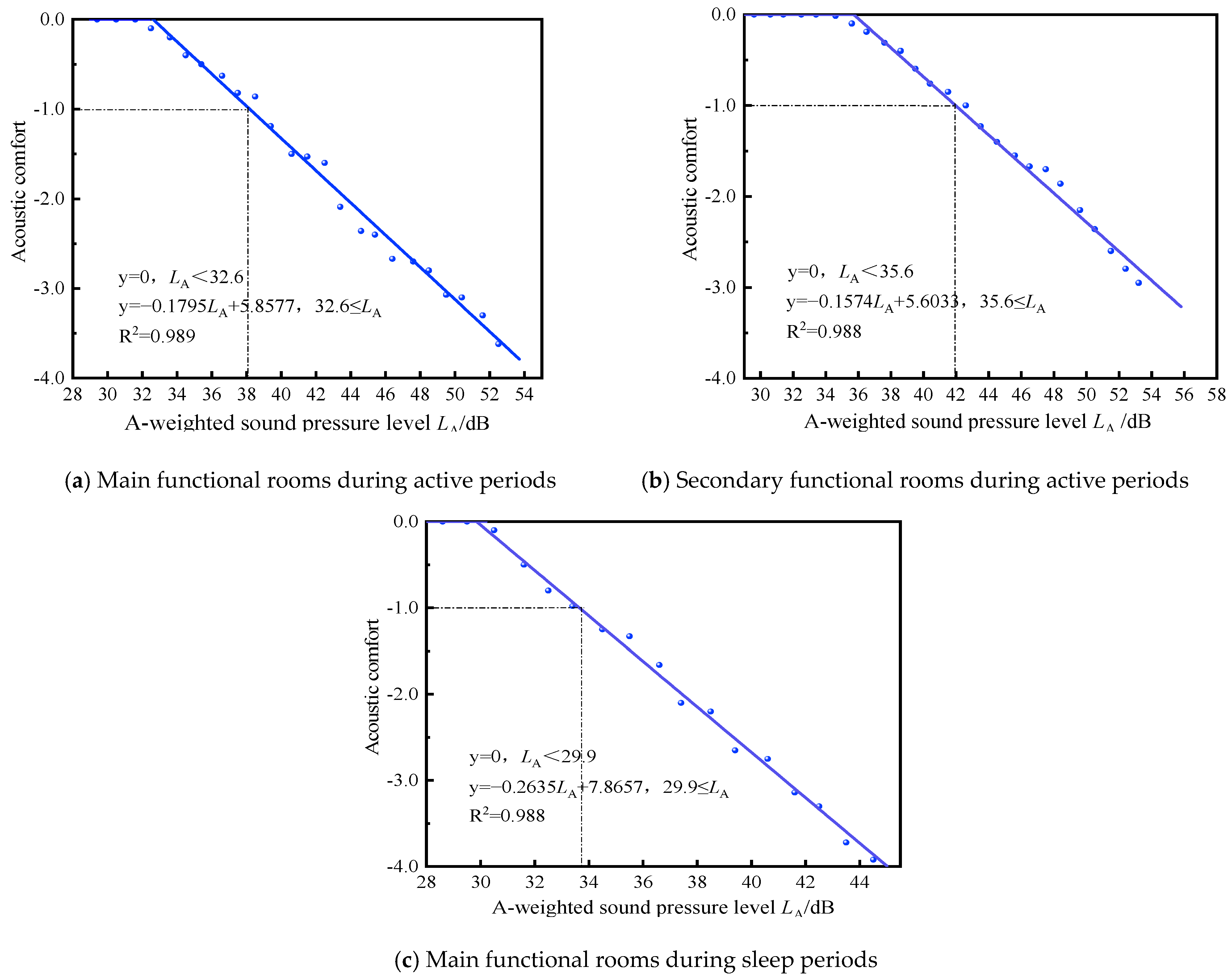
3.2.3. Acoustic Environment

The quantified relationship between acoustic comfort and indoor background noise levels was established by fitting the data, using the average value of each noise level interval as the independent variable and the average value of acoustic comfort voting results as the dependent variable (see Figure 6). The acoustic comfort voting values showed a monotonically decreasing trend as indoor noise levels increased. Based on the fitting results (see

Table 5. Subjective weights of evaluation indicators.

Evaluation Indicators	Subjective Weights
	Main Functional Rooms During Active Periods	Secondary Functional Rooms During Active Periods	Main Functional Rooms During Sleep Periods
Thermal comfort	40.9%	45.6%	34.0%
Lighting comfort	31.7%	33.5%	28.8%
Acoustic comfort	27.4%	20.9%	37.2%

), it was observed that the comfortable noise level range for secondary functional rooms was broader than that for main functional rooms during active periods. For main functional rooms, the comfortable noise level range during sleep periods was significantly broader than that during active periods.

In conclusion, it was evident that the residents’ demands for indoor temperature, illuminance, and noise levels varied across the functional rooms and usage time periods. Therefore, it was suggested to adopt differentiated strategies for the design and control of indoor environment, to effectively enhance indoor environmental comfort and simultaneously achieve energy conservation in buildings, thereby promoting the sustainable development of rural residential environments.

3.3. Weight of Individual Environmental Comfort

Based on the evaluation of the experts for each indicator, the judgment matrix A was obtained as follows:

$${\mathit{A}}_a=\left[\begin{array}{ccc}1.00& 1.35& 1.43\\ 1/1.35& 1.00& 1.21\\ 1/1.43& 1/1.21& 1.00\end{array}\right], {\mathit{A}}_b=\left[\begin{array}{ccc}1.00& 1.59& 1.88\\ 1/1.59& 1.00& 1.87\\ 1/1.88& 1/1.87& 1.00\end{array}\right], {\mathit{A}}_c=\left[\begin{array}{ccc}1.00& 1.20& 0.90\\ 1/1.2& 1.00& 0.79\\ 1/0.9& 1/0.79& 1.00\end{array}\right]$$

(19)

Next, the elements of matrix A were normalized column-wise according to Equations (3) and (4), resulting in the following expression:

$${\mathit{A}}_a=\left[\begin{array}{ccc}0.41& 0.43& 0.39\\ 0.30& 0.31& 0.33\\ 0.29& 0.26& 0.28\end{array}\right], {\mathit{A}}_b=\left[\begin{array}{ccc}0.46& 0.51& 0.40\\ 0.29& 0.32& 0.39\\ 0.25& 0.17& 0.21\end{array}\right], {\mathit{A}}_c=\left[\begin{array}{ccc}0.34& 0.35& 0.34\\ 0.28& 0.29& 0.29\\ 0.38& 0.36& 0.37\end{array}\right]$$

(20)

Then, the subjective weights of each evaluation indicator were determined based on Equation (5), as shown in Table 5.

Furthermore, it can be seen that the judgment matrix A passed the consistency verification based on Equations (6) and (7) (see

Table 6. Consistency verification results.

Verification Indicators	Consistency Verification Indicators
	Main Functional Rooms During Active Periods	Secondary Functional Rooms During Active Periods	Main Functional Rooms During Sleep Periods
CI	0.0010	0.0120	0.0002
CR	0.0017	0.0207	0.0003

).

According to the experts’ scores for each indicator, the evaluation matrix A was established as follows:

$${\mathit{A}}_a=\left[\begin{array}{ccc}3.88& 3.49& 3.01\\ 3.69& 3.64& 2.66\\ ⋮& ⋮& ⋮\\ 4.11& 2.61& 3.01\end{array}\right], {\mathit{A}}_b=\left[\begin{array}{ccc}3.51& 2.61& 1.99\\ 4.00& 3.19& 2.01\\ ⋮& ⋮& ⋮\\ 3.82& 3.65& 2.01\end{array}\right], {\mathit{A}}_c=\left[\begin{array}{ccc}2.64& 1.86& 3.55\\ 3.08& 2.03& 3.41\\ ⋮& ⋮& ⋮\\ 3.01& 2.10& 3.06\end{array}\right]$$

(21)

Next, the original data were standardized according to Equation (10), resulting in the standardized matrix P.

$${\mathit{P}}_a=\left[\begin{array}{ccc}0.17& 0.96& 0.85\\ 0.00& 0.62& 1.00\\ ⋮& ⋮& ⋮\\ 0.39& 0.96& 0.00\end{array}\right], {\mathit{P}}_b=\left[\begin{array}{ccc}0.34& 0.07& 0.93\\ 1.00& 0.59& 1.00\\ ⋮& ⋮& ⋮\\ 0.76& 1.00& 1.00\end{array}\right], {\mathit{P}}_c=\left[\begin{array}{ccc}0.46& 0.00& 1.00\\ 1.00& 0.71& 0.82\\ ⋮& ⋮& ⋮\\ 1.00& 0.91& 0.38\end{array}\right]$$

(22)

Then, based on Equations (11) to (12), the objective weights of each evaluation indicator were obtained, as shown in

Table 7. Objective weights of evaluation indicators.

Evaluation Indicators	Objective Weights
	Main Functional Rooms During Active Periods	Secondary Functional Rooms During Active Periods	Main Functional Rooms During Sleep Periods
Thermal comfort	42.3%	45.0%	33.8%
Lighting comfort	31.7%	36.7%	30.9%
Acoustic comfort	26.0%	18.3%	35.3%

.

Finally, by combining Equation (13) with Table 5 and Table 7, the final weights of each evaluation indicator were obtained, as presented in

Table 8. Combined weights of evaluation indicators.

Evaluation Indicators	Combined Weights
	Main Functional Rooms During Active Periods	Secondary Functional Rooms During Active Periods	Main Functional Rooms During Sleep Periods
Thermal comfort	41.6%	45.3%	33.9%
Lighting comfort	31.7%	35.1%	29.9%
Acoustic comfort	26.7%	19.6%	36.2%

. It was observed that for the main functional rooms during activity periods, the weights for thermal comfort, lighting comfort, and acoustic comfort were 41.6%, 31.7%, and 26.7%, respectively; for the secondary functional rooms during active periods, the corresponding weights were 45.3%, 35.1%, and 19.6%; additionally, for the main functional rooms during sleep periods, the corresponding weights were 33.9%, 29.9%, and 36.2%. Evidently, there are significant differences in the weights of various individual environmental comfort indicators within the comprehensive environmental comfort assessment, and these differences vary depending on the functional rooms and periods of use.

3.4. Evaluation Model for Comprehensive Environmental Comfort

According to the evaluation principle of the penalty substitution synthesis model, as long as the evaluation value of any individual environmental comfort factor reaches its minimum, the evaluation value of the comprehensive environmental comfort also reach its minimum. Given that the established quantitative relationships between individual environmental parameters and individual environmental comfort align with the principles of utility function construction, these relationships could be directly utilized as utility functions. Therefore, based on the comfort evaluation scale set in this paper, the value of L is equal to −4. Thus, the values of the utility function for individual environmental factors should fall within the range of [−4, 0]. This paper introduces the mathematical function “max”, indicating that the values of the utility function for individual environmental factors should satisfy max (−4, yi).

By combining Table 8 and Equation (16), the expression for the comprehensive comfort evaluation model is preliminarily derived as follows:

$$ICEC=-4+{{\displaystyle \prod _{i=1}^n\left[\max \left(-4, y_i\right)+4\right]}}^{{\omega }_i}$$

(23)

where ICEC represents the evaluation value of indoor comprehensive environmental comfort, and $y_{\mathrm{i}}$ represents the utility function of individual environmental factors.

Given that the established quantitative relationships between individual environmental parameters and individual environmental comfort align with the principles of utility function construction, these relationships could be directly utilized as utility functions. By substituting the obtained individual environmental utility functions and weighting coefficients into Equation, the evaluation value of comprehensive environmental comfort can be obtained. However, it is observed that the evaluation values obtained based on Equation (23) significantly differ from those acquired through surveys. Therefore, it is necessary to improve Equation (23) to enhance the predictive accuracy of the model. Based on the changing relationship between the predicted values and the actual values, this paper introduces a Taylor function δ (X) to add a correction term. Selecting X = 0 as the expansion point, the Taylor function is expressed as [48]:

$$\delta \left(X\right)=\delta \left(0\right)+\delta \prime \left(0\right)+{\displaystyle \frac{\delta ″\left(0\right)}{2!}}{X}^2+\dots$$

(24)

Setting ${{\displaystyle \prod _{i=1}^n\left[\max \left(-4, y_i\right)+4\right]}}^{{\omega }_i}=X$, the simplified model for evaluating comprehensive environmental comfort after modification is as follows:

$$ICEC=X-4+\delta \left(X\right)$$

(25)

The evaluation values obtained from field surveys are referred to as actual values, while the evaluation values obtained based on formula Equation (25) are referred to as predicted values. Assuming that m sets of evaluation values are obtained from the survey, the mean square error function based on the least squares method is expressed as:

$$\underset{{\beta }_0, {\beta }_1,{\beta }_2,\dots , {\beta }_n}{\min }={\displaystyle \sum _{i-1}^m\left[{ICEC}_{{\mathrm{actual} \mathrm{value}}_i}{\left(-\left(X_i-4+\delta \left(X_i\right)\right)\right)}^2\right]}$$

(26)

Substituting Equation (24) into Equation (25), we obtain:

$$\underset{{\beta }_0, {\beta }_1,{\beta }_2,\dots , {\beta }_n}{\min }={\displaystyle \sum \left[{\left({IECE}_{{\mathrm{actual} \mathrm{value}}_i}-\left(X_i-4+\delta \left(0\right)+\delta \prime \left(0\right)X_i+\frac{\delta ″\left(0\right)}{2!}{X}_i^2+\dots +\frac{{\delta }^{\left(n\right)}\left(0\right)}{n!}{X}_i^n\right)\right)}^2\right]}$$

(27)

Setting ${\beta }_0=\delta \left(0\right)$, ${\beta }_1=\delta \prime \left(0\right)$,…, ${\beta }_n={\delta }^{\left(n\right)}\left(0\right)$, the above expression becomes:

$$\underset{{\beta }_0, {\beta }_1,{\beta }_2,\dots , {\beta }_n}{\min }={\displaystyle \sum _{i-1}^m\left[{\left({ICEC}_{{\mathrm{actual} \mathrm{value}}_i}-\left(X_i-4+{\beta }_0+{\beta }_1{X}_i+{\beta }_2{X}_i^2+\dots +{\beta }_n{X}_i^n\right)\right)}^2\right]}$$

(28)

Taking partial derivatives with respect to β₀, β₁, β₂, …, β_n respectively, and setting them equal to 0, we obtain:

$$\left\{\begin{array}{l}{\displaystyle \frac{\partial }{\partial {\beta }_0}}{\displaystyle \sum _{i-1}^m\left[{\left({ICEC}_{{\mathrm{actual} \mathrm{value}}_i}-\left(X_i-4+{\beta }_0+{\beta }_1{X}_i+{\beta }_2{X}_i^2+\dots +{\beta }_n{X}_i^n\right)\right)}^2\right]}=0\\ {\displaystyle \frac{\partial }{\partial {\beta }_1}}{\displaystyle \sum _{i-1}^m\left[{\left({ICEC}_{{\mathrm{actual} \mathrm{value}}_i}-\left(X_i-4+{\beta }_0+{\beta }_1{X}_i+{\beta }_2{X}_i^2+\dots +{\beta }_n{X}_i^n\right)\right)}^2\right]}=0\\ \dots \\ {\displaystyle \frac{\partial }{\partial {\beta }_n}}{\displaystyle \sum _{i-1}^m\left[{\left({ICEC}_{{\mathrm{actual} \mathrm{value}}_i}-\left(X_i-4+{\beta }_0+{\beta }_1{X}_i+{\beta }_2{X}_i^2+\dots +{\beta }_n{X}_i^n\right)\right)}^2\right]}=0\end{array}\right.$$

(29)

By transforming and rearranging Equation (29), the above system of equations can be expressed in matrix form as:

$$A\beta =b$$

(30)

where A is the coefficient matrix, β = (β₀, β₁, β₂, …, β_n)^T is the vector of coefficients to be solved, and b is the constant vector).

The elements of the coefficient matrix A and the constant vector b are as follows:

$$a_{jk}={\displaystyle \sum _{i=1}^m{X}_i^{k+j-1}}\left(k=0,1,\dots ,n; j=0,1,\dots ,n\right)$$

(31)

$$b_k={\displaystyle \sum _{i-1}^m{X}_i^k{ICEC}_{\mathrm{actual} \mathrm{value}{e}_i}}-{\displaystyle \sum _{i-1}^m{X}_i^{k+1}}+4{\displaystyle \sum _{i-1}^m{X}_i^k}\left(k=0,1,\dots ,n\right)$$

(32)

When the coefficient matrix A is invertible, the solution for β is obtained as follows:

$$\beta =A^{-1}b$$

(33)

Therefor, the expressions for solving β₀, β₁, β₂, …, β_n are as follows:

$$\left(\begin{array}{l}{\beta }_0\\ {\beta }_1\\ ⋮\\ {\beta }_n\end{array}\right)=A^{-1}\left(\begin{array}{l}{\displaystyle \sum _{i-1}^m{ICEC}_{{\mathrm{actual} \mathrm{value}}_i}-{\displaystyle \sum _{i-1}^m{X}_i}}+4m\\ {\displaystyle \sum _{i-1}^m{X}_i{Y}_i-{\displaystyle \sum _{i-1}^m{X}_i^2}+4{\displaystyle \sum _{i-1}^m{X}_i}}\\ {\displaystyle \sum _{i-1}^m{X}_i^n{Y}_i-{\displaystyle \sum _{i-1}^m{X}_i^{n+1}}+4{\displaystyle \sum _{i-1}^m{X}_i^n}}\end{array}\right)$$

(34)

From the above equation, the values of β₀, β₁, β₂, …, β_n can be determined, and subsequently the expression for the correction term δ (X) can be obtained, as detailed in

Table 9. Correction term δ(X).

Correction Term		Different Types of Rooms
		Main Functional Rooms During Active Periods	Secondary Functional Rooms During Active Periods	Main Functional Rooms During Sleep Periods
δ(X)	Winter	0.3120x2 − 1.0863x	0.2655x2 − 0.9491x	0.3497x2 − 1.3080x
	Summer	0.3288x2 − 1.2290x	0.2737x2 − 1.0744x	0.3501x2 − 1.3706x

.

Based on the above analysis, the general functional expression for the indoor comprehensive environmental comfort evaluation model was as follows:

$$ICEC=-4+X+\delta \left(X\right) \left(X={{\displaystyle \prod _{i=1}^n\left[\max \left(-4,y_i\right)+4\right]}}^{{\omega }_i}\right)$$

(35)

For the main functional rooms during active periods the model was as follows:

$$X={\left[\max \left(-4, y_{a_1}\right)+4\right]}^{0.416}{\left[\max \left(-4, y_{b_1}\right)+4\right]}^{0.317}{\left[\max \left(-4, y_{c_1}\right)+4\right]}^{0.267}$$

(36)

$$y_{a_{1winter}}=-0.0180T^2+0.6100T-4.9866; R^2=0.970$$

(37)

$$y_{a_{1summer}}=-0.0943T^2+4.7517T-60.1560; R^2=0.989$$

(38)

$$y_{b_1}=\left\{\begin{array}{l}0.3409E_L-6.4695, E_L\le 17.5; R^2=0.989\\ -0.6575E_L+11.046, 17.5<E_L; R^2=0.973\end{array}\right.$$

(39)

$$y_{c_1}=\left\{\begin{array}{l}0, x<32.6\\ -0.1795L_A+5.8577, 32.6\le L_A; R^2=0.989\end{array}\right.$$

(40)

where $y_{a_1}$ represents the utility function evaluation value of the indoor temperature in the main functional rooms during active periods, $y_{b_1}$ represents the utility function evaluation value of the indoor temperature in the main functional rooms during active periods, and $y_{c_1}$ represents the utility function evaluation value of the indoor temperature in the main functional rooms during active periods.

For the secondary functional rooms during active periods the model was as follows:

$$X={\left[\max \left(-4, y_{a_2}\right)+4\right]}^{0.453}{\left[\max \left(-4, y_{b_2}\right)+4\right]}^{0.351}{\left[\max \left(-4, y_{c_2}\right)+4\right]}^{0.196}$$

(41)

$$y_{a_{2winter}}=-0.0193T^2+0.6411T-6.0646; R^2=0.980$$

(42)

$$y_{a_{2summer}}=-0.0917T^2+4.6669T-59.5070; R^2=0.987$$

(43)

$$y_{b_2}=\left\{\begin{array}{l}0.3773E_L-6.6325, E_L<17.4; R^2=0.987\\ -0.7240E_L+12.479, 17.4\le E_L; R^2=0.979\end{array}\right.$$

(44)

$$y_{c_2}=\left\{\begin{array}{l}0, L_A<35.6\\ -0.1574L_A+5.6033, 35.6\le L_A; R^2=0.988\end{array}\right.$$

(45)

where $y_{a_2}$ represents the utility function evaluation value of the indoor temperature in the secondary functional rooms during active periods, $y_{b_2}$ represents the utility function evaluation value of the indoor illuminance in the secondary functional rooms during active periods, and $y_{c_2}$ represents the utility function evaluation value of the indoor noise level in the secondary functional rooms during active periods.

For the main functional rooms during sleeping periods the model was as follows:

$$X={\left[\max \left(-4, y_{a_3}\right)+4\right]}^{0.339}{\left[\max \left(-4, y_{b_3}\right)+4\right]}^{0.299}{\left[\max \left(-4, y_{c_3}\right)+4\right]}^{0.362}$$

(46)

$$y_{a_{3winter}}=-0.0187T^2+0.5688T-4.9462; R^2=0.970$$

(47)

$$y_{a_{3summer}}=-0.1310T^2+6.8551T-89.9780; R^2=0.960$$

(48)

$$y_{b_3}=-0.3314E_L-0.0248; R^2=0.989$$

(49)

$$y_{c_3}=\left\{\begin{array}{l}0, L_A<29.9\\ -0.2635L_A+7.8657, 29.9\le L_A; R^2=0.988\end{array}\right.$$

(50)

where $y_{a_3}$ represents the utility function evaluation value of the indoor temperature in the main functional rooms during sleep periods, $y_{b_3}$ represents the utility function evaluation value of the indoor illuminance in the main functional rooms during sleep periods, and $y_{c_3}$ represents the utility function evaluation value of the indoor noise level in the main functional rooms during sleep periods.

It was found that, in specific indoor physical environments, indoor comprehensive environmental comfort could be predicted through a series of representative environmental parameters. This provided a theoretical basis for the scientific evaluation and precise control of indoor environments. During architectural design, designers typically needed to assess and compare multiple design schemes. However, it was difficult to quantitatively assess the differences in the impact of the different design schemes on the comprehensive environmental comfort relying solely on the designer’s personal experience. It is worth mentioning that with the help of this quantitative evaluation model, and using comfort scores as the benchmark, designers could quickly determine the optimal design scheme.

4. Discussion

4.1. Comparison with Previous Results of the Kano Model

Indoor environmental comfort primarily encompasses four aspects: thermal environment, lighting environment, acoustic environment, and air quality, which is a widely accepted theoretical framework. This study conducted an in-depth investigation and analysis of the indoor physical environment of rural dwellings in the Guanzhong Plain of China. The findings revealed that the natural ventilation in these residences was good, air pollution concentrations were low, and the residents had a relatively weak perception of air quality. Furthermore, a quantitative analysis based on the KM showed that air quality belonged to the category of attractive factors within the indoor comprehensive environment. That is, as air quality improved, the comprehensive environmental comfort increased accordingly. However, once needs were met, even moderate performance maintained a high comfort level. Conversely, the comprehensive comfort level did not significantly decrease even if needs remained unmet. Therefore, this study classified indoor air quality as a non-key factor, which was the result of considering regional environmental conditions, building types, and respondent groups. Similar differential findings were also reported in studies by Kim and de Dear, as well as Zhang (see

Table 10. Classification of environmental factors based on the Kano model.

	Environmental Factors
	Thermal	Indoor Air Quality	Luminous	Acoustic
Kim and de Dear [49]	✓	/	/	✓
Zhang [49]	✓	/	/	/
This study	✓	/	✓	✓

Note: “✓“ represents key environmental factors, and “/” represents non-key environmental factors.

).

As shown in Table 10, there were significant differences in the key influencing factors identified across various studies. Through a comparative analysis, the differences were primarily attributed to the following two aspects: first, building types differed significantly. The research data in Kim and de Dear’s study were obtained from CBE’s database, with sample buildings including public administration institutions, research institutions, and educational institutions. Zhang’s study focused on high-speed railway stations in China. However, this study focused on rural dwellings in the Guanzhong Plain of China. Second, the respondent groups differed distinctly. The respondents in the Kim and de Dear study were office workers in Europe and North America, and Zhang’s respondents were Chinese passengers, while the participants in this study were rural residents in the Guanzhong Plain of China. In conclusion, when identifying key environmental factors influencing indoor comprehensive environmental comfort, it was essential to consider factors such as building type and user groups, so as to ensure the accuracy and validity of the research findings.

4.2. Comparison with Previous Comprehensive Evaluation Models

Based on the establishment of quantitative relationships between individual environmental parameters and comfort levels, this study developed a model for evaluating individual environmental comfort. Additionally, it proposes a comprehensive environmental comfort evaluation model based on the utility function method. A summary of comprehensive environmental comfort evaluation models from previous studies is presented in

Table 11. Summary of previous comprehensive environmental comfort evaluation models.

Studies	Research Object	Evaluation Method	Weight Method	Evaluation Model
Cao et al. [50]	Office, teaching building, library	Multivariate linear regression	Regression coefficient	$\begin{array}{l}{S}_T=-0.0063T^2+0.5541T-6.8587\\ S_L=-5\times {10}^{-7}{E}^2+0.0011E-0.106\\ S_A=0.0230L_A+1.382\\ S_{IAQ}=0.0002C_{C{O}_2}+0.244\\ S=0.075+0.31S_T+0.118S_{IAQ}+0.171S_L+0.224S_A\end{array}$
Ncube and Riffat [24]	Office	Multivariate linear regression	Regression coefficient	$\begin{array}{l}{C}_T=100-PPD\\ C_{IAQ}=100-395\times {e^{-15.15\times c{o}_2}}^{-0.25}\\ C_A=100-2\times \left(L_{A-actual}-L_{A-design}\right)\\ C_E=-176.16\times In{\left[In\left(E\right)\right]}^2+738.4\times In\left[In\left(E\right)\right]\\ -690.29\\ C=0.3\times C_T+0.36\times C_{IAQ}+0.16C_E+0.18C_A\end{array}$
Li [23]	Office	Multivariate linear regression	Regression coefficient	$\begin{array}{l}{S}_T=-2.154T^2+108.4T-1274\\ S_L=-0.136E^2+8.568\\ S_A=-1.789L_A+117.6\\ S_{IAQ}=-0.081C_{C{O}_2}+87.47\\ S=0.1525S_T+0.3106S_{IAQ}+0.1511S_L+0.3773S_A-5.5474\end{array}$
Fassi et al. [20]	Classroom	Multivariate linear regression	Regression coefficient	$\begin{array}{l}{\phi }_T=1-{\displaystyle \frac{PPD}{100}}\\ {\phi }_{IAQ}=1-{\displaystyle \frac{1}{2}}\left({\displaystyle \frac{1}{1+e^{3.118-0.00215C_{C{O}_2}}}}-{\displaystyle \frac{1}{1+e^{3.230-0.00117C_{C{O}_2}}}}\right)\\ {\phi }_L=1-{\displaystyle \frac{1}{1+e^{-1.017+0.00558E}}}\\ {\phi }_A=1-{\displaystyle \frac{1}{1+e^{9.540-0.134L_A}}}\\ \phi =0.33{\phi }_T+0.26{\phi }_A+0.25{\phi }_L+0.16{\phi }_{IAQ}\end{array}$
Yang and Mark [22]	Classroom	Multivariate logistic regression	Regression coefficient	$\begin{array}{l}{S}_T=-0.0117T^2+0.5979T-6.878\\ S_L=-4.838\times {10}^{-7}{E}^2+8.179E-0.4833\\ S_A=0.01216L_A+1.452\\ S_{IAQ}=0.0004242C_{C{O}_2}+0.9756\\ S=0.3177S_T+0.1629S_{IAQ}+0.2386S_L+0.2808S_A\end{array}$
Lai et al. [25]	High-rise residential	Multivariate logistic regression	Regression coefficient	$\begin{array}{l}{\phi }_T=0.95e^{-0.2179\times {\left(2.2PMV-0.15\right)}^2-0.03353\times {\left(2.2PMV-0.15\right)}^4}\\ {\phi }_{IAQ}=1-{\displaystyle \frac{1}{1+e^{45.24-0.0257C_{C{O}_2}}}}\\ {\phi }_L=1-{\displaystyle \frac{1}{1+e^{-14.13+0.9058E}}}\\ {\phi }_A=1-{\displaystyle \frac{1}{1+e^{23.75-0.2986L_A}}}\\ \phi =1-{\displaystyle \frac{1}{1+e^{-33.63+22.05{\phi }_T+1.609{\phi }_{IAQ}+11.77{\phi }_L+21.86{\phi }_A}}}\end{array}$
Catalina and Iordache [21]	Classroom	Multivariate linear regression	Regression coefficient	$\begin{array}{l}{\phi }_T=\left\{\begin{array}{l}28.57T-514, T\le 21.5\\ 800-28.57T, T>21.5\end{array}\right.\\ {\phi }_{IAQ}=3.125C_{{CO}_2}-12.5\\ {\phi }_L=0.33E\\ {\phi }_A=-3.33L_A+200\\ \phi ={\displaystyle \frac{{\phi }_T+{\phi }_{IAQ}+{\phi }_A+{\phi }_L}{4}}\end{array}$

Note: T, E, L_A, and $C_{{CO}_2}$ represent temperature, illuminance, noise level, and carbon dioxide concentration, respectively; S, C, and $\phi$ denote satisfaction, comfort, and acceptability, respectively.

. Comparing prior models with the one proposed in this study, it was found that direct comparison is challenging due to differences in key environmental factors, building types, and surveyed populations across different studies. However, previous comprehensive comfort assessment models primarily focused on office and educational buildings, while research on residential buildings, particularly rural dwellings, was significantly lacking. Moreover, these models typically neglected two critical aspects: (1) the veto effect of individual environmental comfort, and (2) the differentiated demands of residents for the indoor physical environment. Additionally, previous studies typically determined weights based on regression coefficients. This method overly relies on data quality, lacks subjective judgment, and is limited to linear assumptions about variable relationships. In contrast, this study adopted a combination of the AHP and EWM, effectively avoiding these issues and further ensuring the accuracy of the research findings.

4.3. Application of the Comprehensive Comfort Evaluation Model

In specific indoor physical environments, the comfort level of the indoor comprehensive environment can be predicted through representative environmental parameters. This provides a theoretical basis for the scientific evaluation and precise regulation of indoor environments. In practice, designers specializing in the optimization of indoor physical environments often need to evaluate and compare multiple design schemes. However, relying solely on personal experience makes it difficult to accurately quantify the differential impacts of various design schemes on indoor comprehensive environmental comfort. By introducing a quantitative evaluation model for indoor environmental comfort and utilizing composite scores as an objective benchmark, designers can quickly and efficiently identify the optimal design solution. This approach not only enhances the objectivity and accuracy of design decisions but also provides reliable quantitative support for the optimization of indoor environments.

5. Conclusions

This study focused on the rural residences of the Guanzhong Plain as the research subject and conducted an evaluation of indoor comprehensive environmental comfort based on various physical environmental factors. The main conclusions were as follows:

(1)

Based on the subjective evaluation characteristics of indoor environmental comfort and the principles of multi-factor comprehensive evaluation, a comprehensive environmental comfort evaluation method utilizing the utility function approach was proposed.

(2)

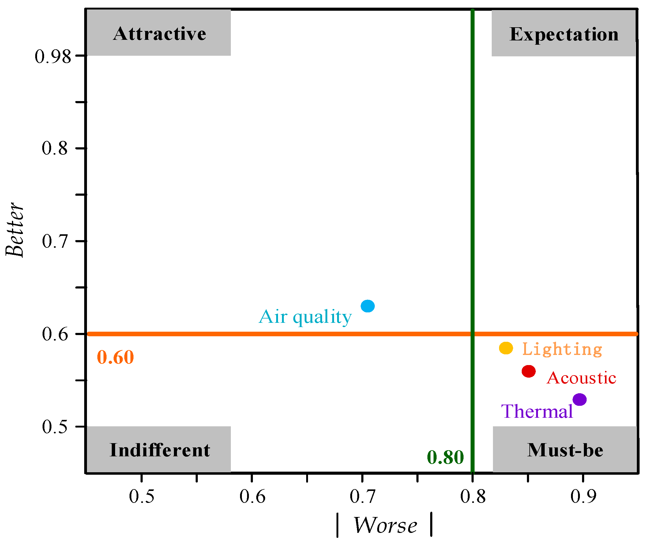
Through a quantitative analysis using the Kano model, the thermal, light, and acoustic environments were identified as the key factors affecting comprehensive indoor environmental comfort, while air quality was a non-key factor.

(3)

The weights of different individual environmental comfort factors in the comprehensive environmental comfort varied, with differences further influenced by room attributes and usage time periods.

(4)

Quantitative relationships between comfort and temperature, illuminance, and noise levels were established, and the weights of individual environmental factors were determined, based on the perspective of categorizing functional rooms and usage time periods.

(5)

A quantitative evaluation model for indoor comprehensive environmental comfort that considered the one-vote veto characteristics and differentiated demands was proposed based on the penalty substitution synthesis method.

References

1. Abdel-Salam, M.M.M. Indoor exposure of elderly to air pollutants in residential buildings in Alexandria, Egypt. Build. Environ. 2019, 7, 109221. [Google Scholar] [CrossRef]
2. Indraganti, M.; Boussaa, D. An adaptive relationship of thermal comfort for the Gulf Cooperation Council (GCC) Countries: The case of offices in Qatar. Energy Build. 2018, 159, 201–212. [Google Scholar] [CrossRef]
3. Rajan, K.; Rijal, H.B.; Shukuya, M.; Yoshida, K. An in-situ study on occupants’ behaviors for adaptive thermal comfort in a Japanese HEMS condominium. Build. Eng. 2018, 19, 402–411. [Google Scholar]
4. Rijal, H.B. Thermal adaptation of buildings and people for energy saving in extreme cold climate of Nepal. Build. Environ. 2021, 230, 110551. [Google Scholar] [CrossRef]
5. Fan, X.N.; Zhao, Q.; Sang, G.C.; Zhu, Y.Y. Numerical Study on the Suitability of Passive Solar Heating Technology Based on Differentiated Thermal Comfort Demand. Comput. Model. Eng. Sci. 2022, 132, 627–660. [Google Scholar] [CrossRef]
6. Mohd Husini, E.; Arabi, F.; Ossen Dilshan, R.; Kandar, M.Z.; Mat Lajis, N. Daylight in Office Buildings in Malaysia: A Pilot Study on Occupants’ Satisfaction and Luminous Environment. Spaces Flows Int. Urban Extra Urban Stud. 2008, 3, 662–677. [Google Scholar] [CrossRef]
7. Zhu, C.H.; Li, N.P.; Re, D.; Guan, J. Uncertainty in indoor air quality and grey system method. Build. Environ. 2007, 42, 1711–1717. [Google Scholar] [CrossRef]
8. Mui, K.W.; Wong, L.T. A method of assessing the acceptability of noise levels in air conditioned offices. Build. Serv. Eng. Res. Technol. 2006, 27, 249–254. [Google Scholar] [CrossRef]
9. Liu, H.M.; He, H.; Qin, J.J. Does background sounds distort concentration and verbal reasoning performance in open-plan office. Appl. Acoust. 2021, 172, 107577. [Google Scholar] [CrossRef]
10. Washita, G.; Kimura, K.; Tanabe, S.; Yoshizawa, S.; Ikeda, K. Indoor air quality assessment based on human olfactory sensation. J. Archit. Plan. Environ. 1990, 410, 9–19. [Google Scholar]
11. Li, W.M.; Lee, S.C.; Chan, L.Y. Indoor air quality at nine shopping malls in Hong Kong. Sci. Total Environ. 2001, 273, 27–40. [Google Scholar] [CrossRef]
12. Djamila, H.; Chu, C.M.; Kumaresan, S. Field study of thermal comfort in residential buildings in the equatorial hot-humid climate of Malaysia. Build. Environ. 2013, 62, 133–142. [Google Scholar] [CrossRef]
13. Yu, W.; Li, B.Z.; Yao, R.M.; Wang, D.; Li, K.T. A study of thermal comfort in residential buildings on the Tibetan Plateau, China. Build. Environ. 2017, 119, 71–86. [Google Scholar] [CrossRef]
14. Guo, T.M.; Hu, S.T.; Liu, T.M. Research on the influence factors of indoor light environment comfort within asymptomatic altitude reaction. Build. Sci. 2016, 32, 39–44. [Google Scholar]
15. de Boer, J.B.F. Indoor Lighting; Light Industry Press: Beijing, China, 1989. [Google Scholar]
16. Fanger, P.O. Theral Comfort; Krieger Publishing Company: Malabar, FL, USA, 1982. [Google Scholar]
17. Clausen, G. A comparative study of discomfort caused by indoor air pollution, thermal load and noise. Indoor Air. 2021, 3, 255–262. [Google Scholar] [CrossRef]
18. Li, Z.; Zhang, Q.W.; Fan, F.; Shen, S.Z. A comprehensive comfort assessment method for indoor environmental quality in university open-plan offices in severe cold regions. Build. Environ. 2021, 197, 107845. [Google Scholar] [CrossRef]
19. Guo, T.M.; Hu, S.T.; Liu, G.D. Evaluation model of specific indoor environment overall comfort based on effective-function method. Energies 2017, 10, 1634. [Google Scholar] [CrossRef]
20. Fassio, F.; Fanchiotti, A.; De Lieto Vollaro, R. Linear, non-linear and alternative algorithms in the correlation of IEQ factors with global comfort: A case study. Sustainablity 2014, 6, 8113–8127. [Google Scholar] [CrossRef]
21. Mihai, T.; Iordache, V. Determining the indoor environment quality for an educational building. Energy Proc. 2016, 85, 566–574. [Google Scholar] [CrossRef]
22. Yang, D.; Mak, C.M. Relationships between indoor environmental quality and environmental factors in university classrooms. Build. Environ. 2020, 186, 107331. [Google Scholar] [CrossRef]
23. Li, S.M. Study on Environmental Quality Evaluation Model of Office Building. Master’s Thesis, Guangzhou University, Guangzhou, China, 2018. [Google Scholar]
24. Ncube, M.; Riffat, S. Developing an indoor environment quality tool for assessment of mechanically ventilated office buildings in the UK—A preliminary study. Build. Environ. 2012, 53, 26–33. [Google Scholar] [CrossRef]
25. Lai, A.C.K.; Mui, K.W.; Wong, L.T.; Law, L.Y. An evaluation model for indoor environmental quality (IEQ) acceptance in residential buildings. Energy Build. 2009, 41, 930–936. [Google Scholar] [CrossRef]
26. Wei, N.; Guo, Y.; Feng, X.Y.; Cao, X.Y.; Su, L.J. Study on the thermal environment of rural residential buildings in winter in the Guanzhong region of Shaanxi. Ecol. Econ. 2023, 1, 79–90. [Google Scholar]
27. Ji, T.T.; Zhang, T.; Fukuda, H. Thermal Comfort Research on the Rural Elderly in the Guanzhong Region: A Comparative Analysis Based on Age Stratification of Residential Environments. Sustainability 2024, 16, 6101. [Google Scholar] [CrossRef]
28. ISO 7726; Thermal Environmental Conditions for Human Occupancy. International Standardization Organization: Geneva, Switzerland, 1985.
29. Liu, Y.S.; Yang, C.H.; Huang, K.K.; Liu, Y.P. A multi-factor selection and fusion method through the CNN-LSTM network for dynamic Price forecasting. J. Jpn. Soc. Qual. Control 2023, 11, 1132. [Google Scholar] [CrossRef]
30. Fan, C.H.; Chen, Y.; Zhang, L.; Wu, W.J.; Ling, B.; Tian, S.J. Using fuzzy comprehensive evaluation to assess the competency of full-time water conservancy emergency rescue teams. Mathematics 2021, 10, 2111. [Google Scholar] [CrossRef]
31. Zheng, G.Z.; Li, K.; Bu, W.T.; Wang, Y.J. Fuzzy comprehensive evaluation of human physiological state in indoor high temperature environments. Build. Environ. 2019, 150, 108–118. [Google Scholar] [CrossRef]
32. Pazouki, M.; Rezaie, K.; Bozorgi Amiri, A. A fuzzy robust multi-objective optimization model for building energy retrofit considering utility function: A university building case study. Energy Build. 2021, 241, 110933. [Google Scholar] [CrossRef]
33. Tong, H.P.; Krishna Kumar, T.; Huang, Y.X. Multivariate Statistical Analysis and Data Analysis; Wiley Online Library: Hoboken, NJ, USA, 2011. [Google Scholar]
34. Li, J.P.; Xie, B.C. Multivariate Statistical Analysis; China Renmin University Press: Beijing, China, 2008. [Google Scholar]
35. Liu, S.F.J.; Yang, Y.; Liu, S. Grey System: Thinking, Methods, and Models with Applications; Wiley Online Library: Hoboken, NJ, USA, 2015. [Google Scholar]
36. Baymani, M.; Effati, S.; Niazmand, H.; Kerayechian, A. Kerayechian Artificial neural network method for solving the Navier–Stokes equations. Neural Comput. Appl. 2014, 26, 765–773. [Google Scholar] [CrossRef]
37. Sun, X.D.; Li, Z.; Chen, F.M. Research on multiple attribute synthetical evaluation methods based on artificial neural network. J. Zhengzhou Univ. Light Ind. Nat. Sci. 2003, 18, 11–14. [Google Scholar]
38. Liu, L.L.; Dou, Y.M.; Qiao, J.G. Evaluation method of highway plant slope based on rough set theory and analytic hierarchy process: A case study in Taihang mountain, Hebei, China. Mathematics 2022, 10, 1264. [Google Scholar] [CrossRef]
39. Fan, X.N.; Guo, Y.; Zhao, Q.; Zhu, Y.Y. Structural optimization and application research of alkali-activated slag ceramsite compound insulation block based on finite element method. Mathematics 2021, 9, 2488. [Google Scholar] [CrossRef]
40. Wang, Q.; Liu, Y.F.; Zhang, X.D.; Fu, H.C.; Niu, C.C. Study on an AHP-Entropy-ANFIS model for the prediction of the unfrozen water content of sodium-bicarbonate-type salinization frozen soil. Mathematics 2020, 8, 1209. [Google Scholar] [CrossRef]
41. Liu, J.; Yu, S.H.; Chu, J.J. The comfort evaluation in civil aircraft cabin based on objective and subjective weighting method. J. Graph. 2017, 38, 192–197. [Google Scholar]
42. Kano, N.; Seraku, N.; Takahashi, F. Attractive quality and must-be quality. J. Jpn. Soc. Qual. Control 1984, 14, 39–48. [Google Scholar]
43. Kim, J.; de Dear, R. Nonlinear relationships between individual IEQ factors and overall workspace satisfaction. Build. Environ. 2012, 49, 33–40. [Google Scholar] [CrossRef]
44. Zhang, Y.C. Research on Interaction Effect of Thermal, Light and Acoustic Environment on Human Comfort in Waiting Area of High-Speed Railway Station; Beijing Jiaotong University: Beijing, China, 2021. [Google Scholar]
45. Geng, Y.; Yu, J.; Lin, B.; Wang, Z.; Huang, Y. Impact of individual IEQ factors on passengers’ overall satisfaction in Chinese airport terminals. Build. Environ. 2017, 12, 241–249. [Google Scholar] [CrossRef]
46. Timko, M. An experiment in continuous analysis. J. Manag. Qual. Cent. 1993, 2, 17–20. [Google Scholar]
47. GB 50034-2024; Standard for Lighting Design of Buildings. MOHURD, China Architecture & Building Press: Beijing, China, 2013.
48. Wu, S.H.; Adil Khan, M. Refinements of majorization inequality involving convex functions via Taylor’s theorem with mean value form of the remainder. Mathematics 2019, 7, 663. [Google Scholar] [CrossRef]
49. Kim, J.; de Dear, R. Impact of different building ventilation modes on occupant expectations of the main IEQ factors. Build. Environ. 2012, 57, 184–193. [Google Scholar] [CrossRef]
50. Cao, B.; Qin, Q.; Zhu, Y.; Li, H.; Hu, H.; Deng, G. Development of a multivariate regression model for overall satisfaction in public buildings based on field studies in Beijing and Shanghai. Build. Environ. 2012, 47, 394–399. [Google Scholar] [CrossRef]
Figure 1. Main calculation steps of Kano model.
Mathematics 13 01000 g001
Figure 2. Better–|Worse| four-quadrant diagram.
Mathematics 13 01000 g002
Figure 3. Relationship between thermal comfort votes and winter indoor temperature.
Mathematics 13 01000 g003
Figure 4. Relationship between thermal comfort votes and summer indoor temperature.
Mathematics 13 01000 g004
Figure 5. Relationship between light comfort votes and indoor illuminance.
Mathematics 13 01000 g005
Figure 6. Relationship between acoustic comfort votes and indoor noise.
Mathematics 13 01000 g006