
Bifurcation, Quasi-Periodic, Chaotic Pattern, and Soliton Solutions to Dual-Mode Gardner Equation

Abstract
1. Introduction
2. Traveling Wave System
3. Bifurcation and Phase Portrait
- (a)
- A solitary solution corresponding to a homoclinic trajectory when .
- (b)
- A kink (or anti-kink) solution corresponding to a heteroclinic trajectory when .
- (c)
- A periodic solution corresponding to the periodic phase trajectory.
- 1.
- If , which is equivalent to , then Equation (13) has a unique solution, . Consequently, the system in Equation (7a,b) has a single equilibrium point, . To classify the nature of this point, we apply Theorem 1. Direct calculations yield . The point is classified as either a center point if or a saddle point if . The value of the parameter q at the equilibrium point is calculated, resulting in . Figure 1 illustrates the phase portrait of the system (7a,b) for , representing the scenario in which the system has a single equilibrium point. We conclude that when , all phase trajectories of the system are bounded and periodic, and are classified as for all , as depicted in Figure 1a. Conversely, when , all phase trajectories of the system (7a,b) are unbounded for all possible values of .
- 2.
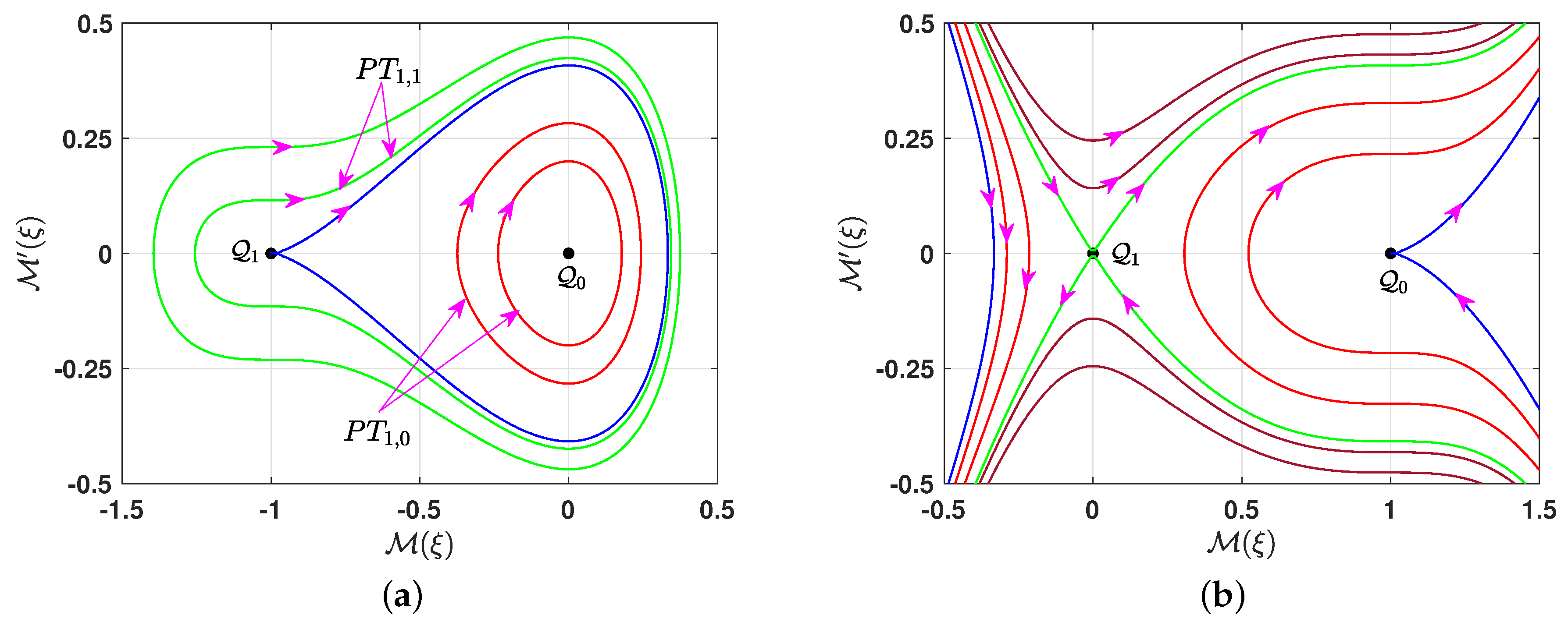
- When , this condition corresponds to , where . In this case, Equation (13) yields two solutions: and . As a result, the system (7a,b) possesses two equilibrium points: and . Theorem 1 is applied to classify these points. Direct calculations yieldHence, the equilibrium point is a cusp point, and is a center point if or a saddle point if . The phase portrait for the system (7a,b) in this case is shown in Figure 2. We compute the value of the parameter q at the following equilibrium points: and . We briefly describe the phase portrait in this case. When , all phase trajectories are bounded and periodic, varying according to the values of the parameter q, as shown in Figure 2a. There are two families of periodic trajectories: one characterized by for in green, and the other by for in red. Additionally, the blue trajectory passing through the cusp point typically exhibits periodic behavior, especially near the equilibrium point. On the other hand, if , all phase trajectories of the system (7a,b) are unbounded, as shown in Figure 2b.
- 3.
- If , which is equivalent to , then Equation (13) has three real solutions, . Consequently, the system (7a,b) has three equilibrium points: and . The Lagrange Theorem 1 is employed to classify the equilibrium points; hence, we haveAlso, we compute the value of q at the following points:which are sufficient to give a short description of the phase portrait. Let us now consider the next two cases, in which is either positive or negative:
- Case A: If , the condition yields or :
- (a)
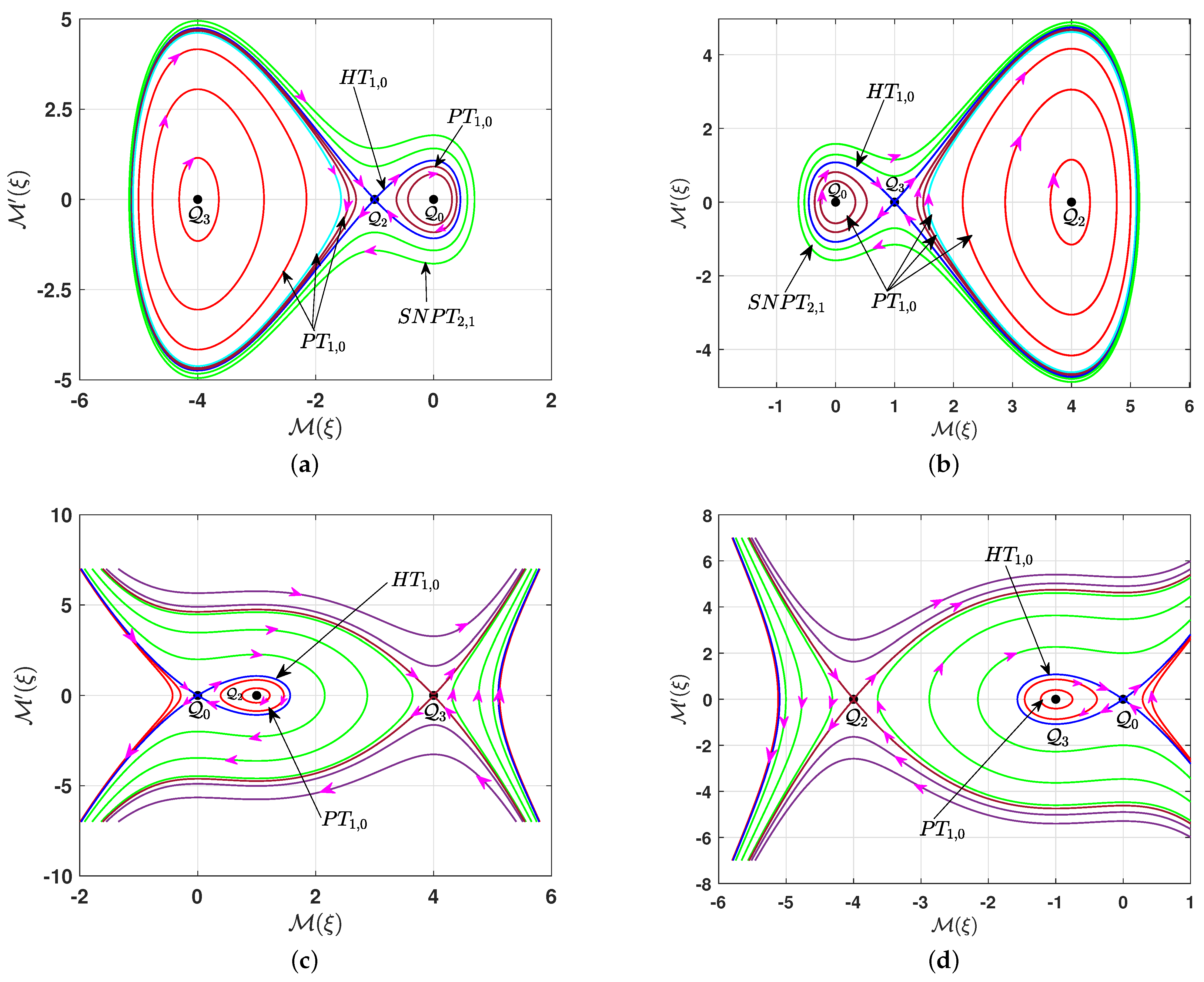
- If , and , the equilibrium point is a center point, while is a saddle point and is a center point. Figure 3a depicts the phase portrait for the system (7a,b) in this case. It consists of several types of bounded trajectories, depending on the values of the parameter q. There is a family of super-periodic trajectories in green, characterized by for , two brown families of periodic trajectories around the center point , characterized by for , a family of red periodic trajectories around the center point , characterized by for , and a single cyan periodic trajectory for . Additionally, there are two homoclinic trajectories in blue for , which is characterized by .
- (b)
- On the other hand, if , and , then is a center point, is a center point, and is a saddle point. The phase portrait for this case is shown in Figure 3b. All the trajectories are bounded and categorized into different types based on the value of the parameter q. A similar phase description can be provided as in (a).
- (c)
- If , and , the equilibrium point is a saddle point, while is a center point and is a saddle point. The phase portrait for this case is illustrated in Figure 3c. All the phase trajectories are unbounded, except for the family of periodic red trajectories for , which is characterized by . This family is enclosed within a homoclinic trajectory in blue for , which is characterized by .
- (d)
- If , and , the equilibrium point is a saddle point, while is a saddle point and is a center point. The phase portrait for this case is shown in Figure 3d. A similar phase description can be provided as in (c).
- Case B: If , then the condition holds automatically. Thus, we proceed to consider the following possible cases:
- (a)
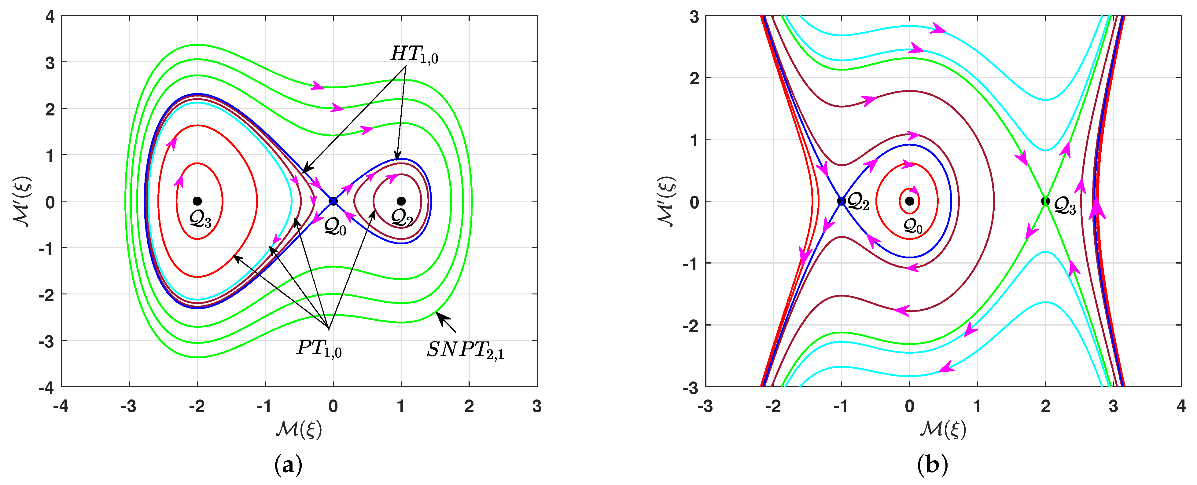
- If , and is a nonzero real number, the equilibrium point is a saddle point while and are center points. The phase portrait for the system (7a,b) corresponding to this case is illustrated in Figure 4a. All the phase trajectories are bounded, and their type depends on the value of the parameter q. There is a family of periodic red trajectories around the center point for , and two periodic families of brown trajectories surrounding the two center points and for , situated within the two homoclinic orbits (blue) at . Additionally, there is a single periodic trajectory (cyan) for . All these periodic trajectories are characterized by . Furthermore, for , there is a green family of super-periodic trajectories characterized by .
- (b)
- If , and is a nonzero real number, the equilibrium point is a center point while both equilibrium points are saddle points. The phase portrait for this case is depicted in Figure 4b. All the phase trajectories are unbounded, except for a family of red periodic trajectories around the center point when . This family lies within the homoclinic orbit (blue) at .
4. Solutions
4.1. Periodic Solutions
- (a)
- The parameter conditions in Case 1 indicate that the polynomial (12) has two real roots, denoted as , where , and two complex conjugate roots, denoted as , where * denotes the complex conjugate. Thus, it can be expressed as . The interval for the real solution is . Assuming , integrating both sides of Equation (11) yields a new solution to Equation (2) of the formwhere , , and . The solution (15) is periodic, with a period given by , where denotes the complete elliptic integral of the first kind [49].The solutions corresponding to Case 2, Case 3, Case 5, Case 7, and Case 12 in Table 1 are identical to the solution (15), differing only in their arguments. This difference arises because the roots of the polynomial change with the parameter constraints, while the sign of the leading order of the polynomial remains fixed.
- (B)
- The parameter conditions in Case 4, Case 8, and Case 13 indicate that the polynomial (12) has four real zeros, denoted as for , satisfying . Thus, it is written as . The intervals of the real solutions are . For , we assume and integrate both sides of Equation (11). Consequently, we obtain a novel periodic solution to Equation (2) of the formwhere . The period of the solution (16) is , where is a complete elliptic integral of the first kind [49]. The solution (16) corresponds to the left family of periodic trajectories, as illustrated in Figure 3a,b. On the other hand, if , we assume that . Consequently, integrating both sides of Equation (11) yieldswhich is a new periodic solution to Equation (2) with period . The solution (17) corresponds to the right family of periodic trajectories, as shown in Figure 3a,b.Note that for fixed values of the parameters , and q, two distinct solutions arise, depending on the differences in the intervals of real solutions. Hence, employing such intervals is crucial.
- (c)
- The parameter conditions in Case 6 and Case 9 indicate that the polynomial (12) has one double root at the origin and two simple roots given by . In Case 6, these roots satisfy , while in Case 9, . The polynomial (12) can be expressed as . The interval of real propagation is for Case 6 and for Case 9. Postulating in both cases and integrating both sides of Equation (11), we obtain
- (d)
- Cases 10, 11, and 15 justify the existence of four real zeros of the polynomial, namely , with . It is worth mentioning that the values of these roots vary from case to case due to their dependence on the polynomial coefficients. The polynomial (12) is expressed as . The intervals of the real solutions are given by . We restrict ourselves to , as this interval corresponds to periodic trajectories, whereas the other intervals describe unbounded trajectories. Integrating both sides of Equation (11) under the assumption (11) that yieldswhere . The solution (19) characterizes a new solution to Equation (2), with a period given by .
4.2. Super-Periodic Solutions
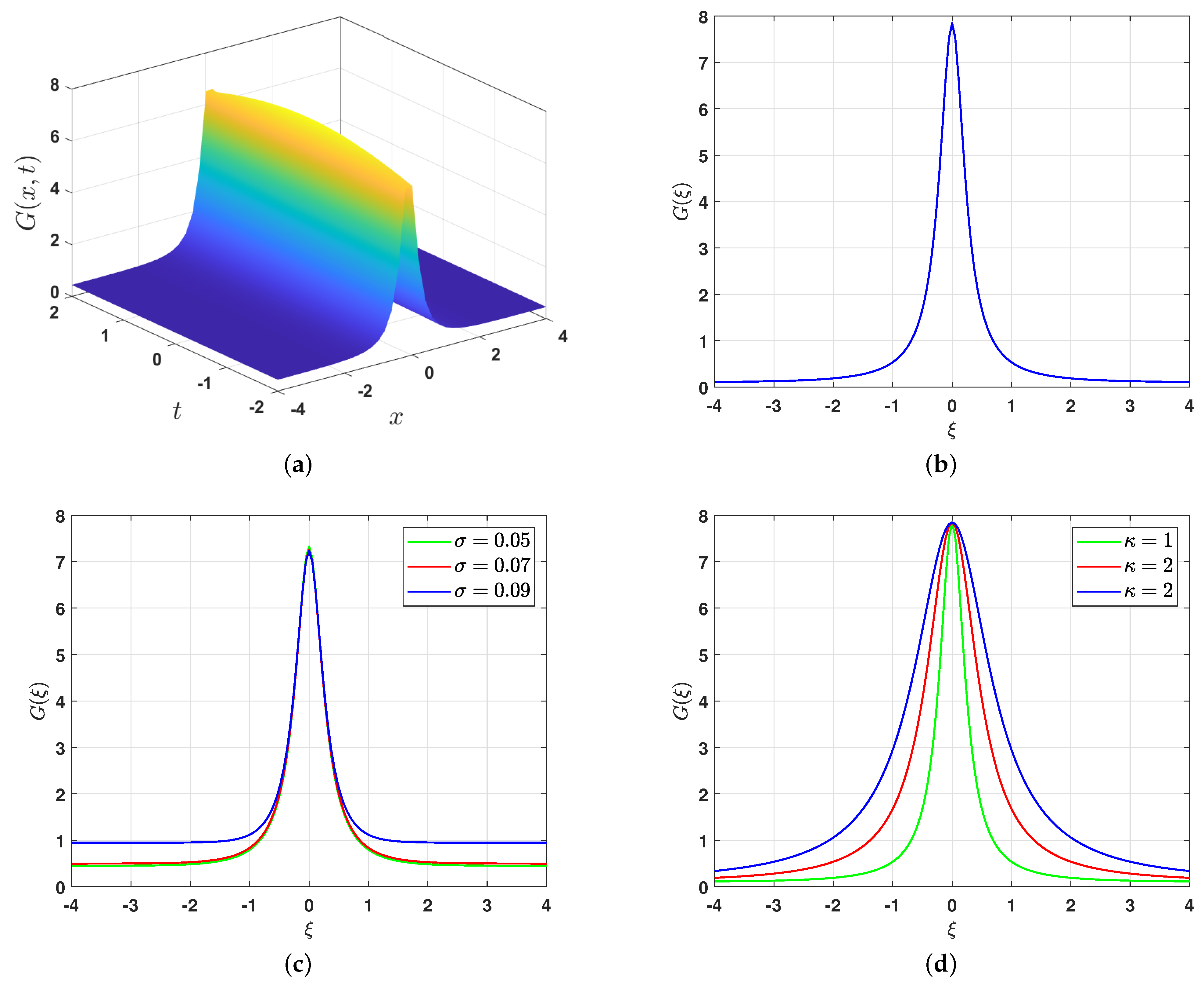
4.3. Solitary Solutions
- (a)
- (b)
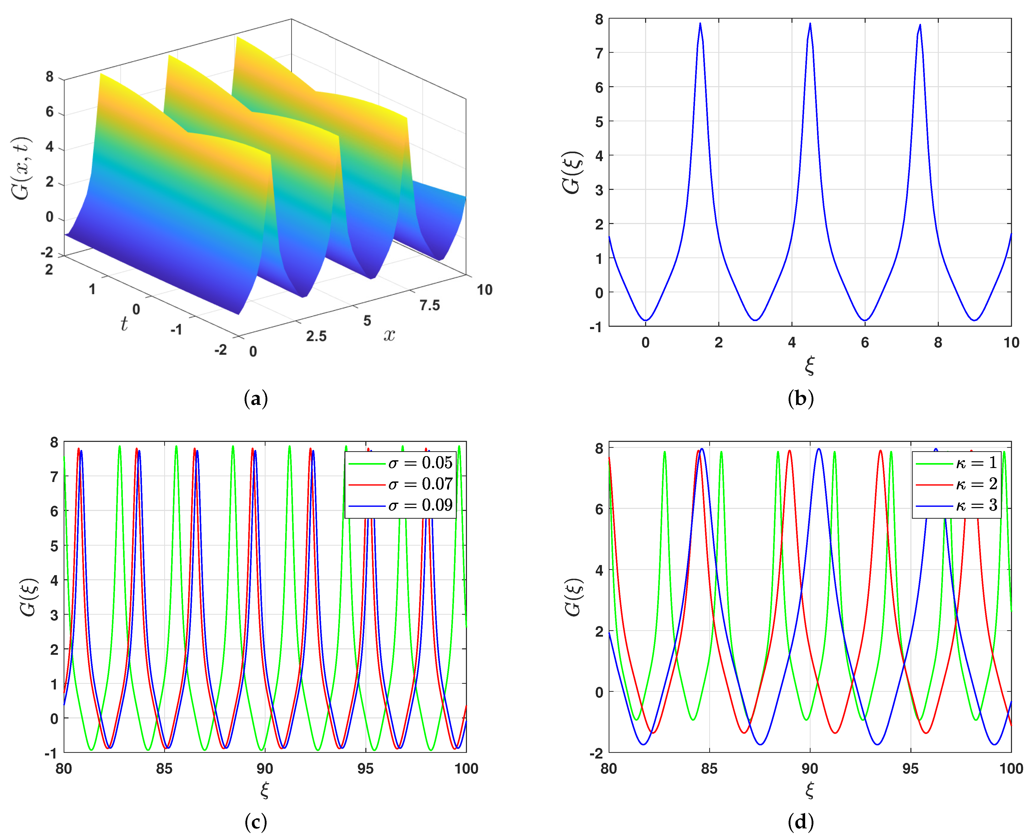
5. Physical Interpretation
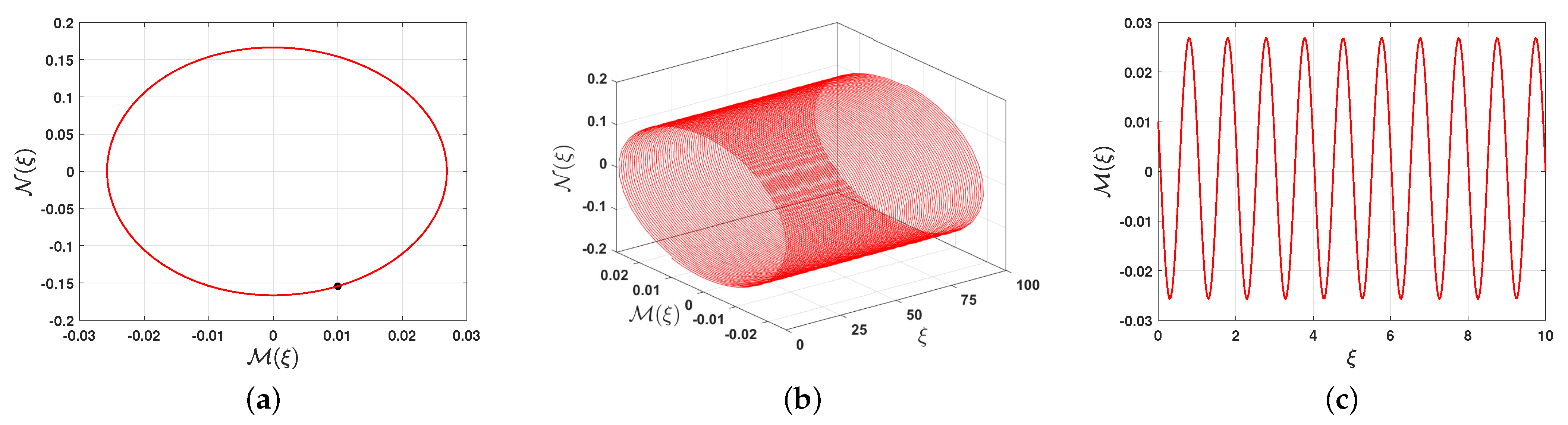
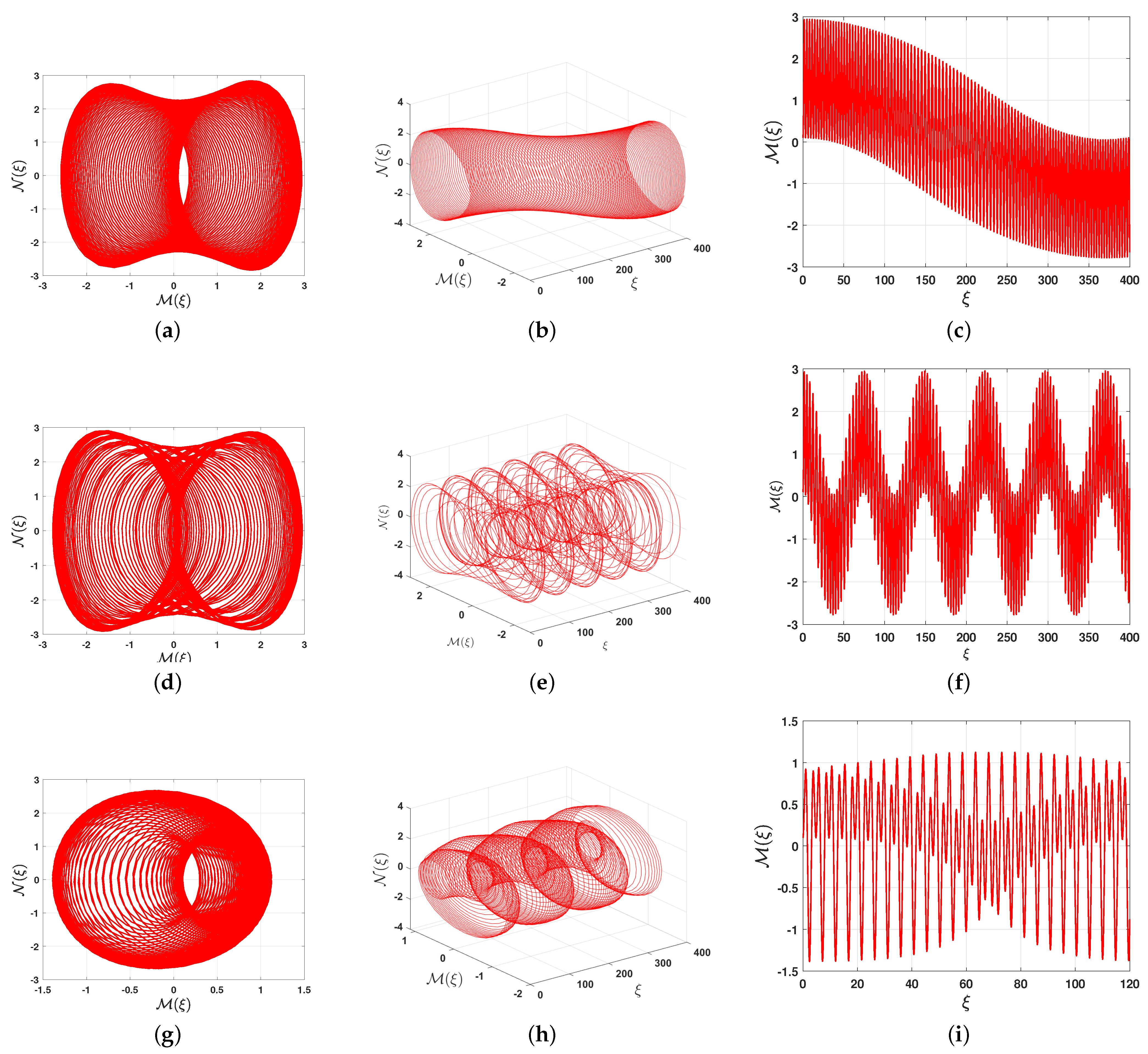
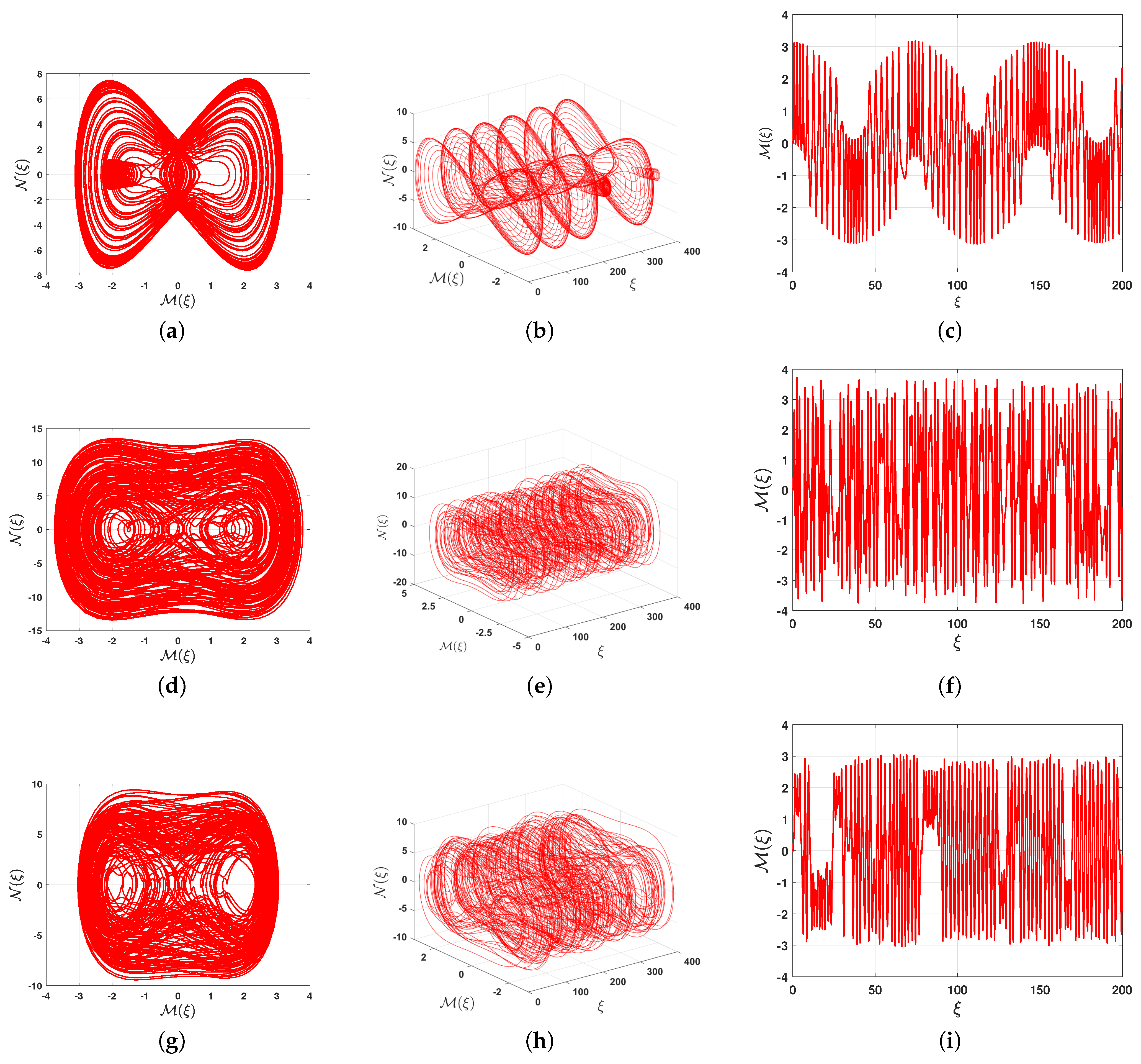
6. Quasi-Periodic Behavior
7. Conclusions
- (a)
- This approach enables us to classify the solutions before explicitly determining them by linking the solution types to the phase trajectories, as stated in Lemma 1. In other words, it provides the existence conditions for periodic, super-periodic, and solitary solutions, as shown in Table 1, Table 2, and Table 3, respectively.
- (b)
- This approach allows us to construct real (non-complex) solutions by considering the intervals of real wave propagation. Moreover, the significance of these intervals cannot be overlooked, as different intervals of real wave propagation yield different solutions. In other words, even under the same parameter conditions, distinct solutions arise due to variations in the intervals of real wave propagation.
- (c)
- This approach allows us to isolate unbounded solutions, which are less relevant in real-world applications. However, it is worth mentioning that these solutions can be computed using the same procedures as bounded solutions.
Funding
Data Availability Statement
Conflicts of Interest
References
- Gao, W.; Ismael, H.F.; Bulut, H.; Baskonus, H.M. Instability modulation for the (2 + 1)-dimension paraxial wave equation and its new optical soliton solutions in Kerr media. Phys. Scr. 2020, 95, 035207. [Google Scholar] [CrossRef]
- Fan, F.C.; Xu, Z.G.; Shi, S.Y. Soliton, breather, rogue wave and continuum limit for the spatial discrete Hirota equation by Darboux–Bäcklund transformation. Nonlinear Dyn. 2023, 111, 10393–10405. [Google Scholar] [CrossRef]
- Ablowitz, M.J.; Clarkson, P.A. Solitons, Nonlinear Evolution Equations and Inverse Scattering; Cambridge University Press: Cambridge, UK, 1991. [Google Scholar]
- Hirota, R. Exact N-soliton solutions of the wave equation of long waves in shallow-water and in nonlinear lattices. J. Math. Phys. 1973, 14, 810–814. [Google Scholar] [CrossRef]
- Alomair, A.; Al Naim, A.S.; Bekir, A. Exploration of Soliton Solutions to the Special Korteweg–De Vries Equation with a Stability Analysis and Modulation Instability. Mathematics 2024, 13, 54. [Google Scholar] [CrossRef]
- Matveev, V.B.; Salle, M.A. Darboux Transformations and Solitons; Springer Series in Nonlinear Dynamics; Springer: Berlin/Heidelberg, Germany, 1991. [Google Scholar]
- Konopelchenko, B.; Rogers, C. Bäcklund and reciprocal transformations: Gauge connections. Math. Sci. Eng. 1992, 185, 317–362. [Google Scholar]
- Rashedi, K.A.; Almusawa, M.Y.; Almusawa, H.; Alshammari, T.S.; Almarashi, A. Applications of Riccati–Bernoulli and Bäcklund Methods to the Kuralay-II System in Nonlinear Sciences. Mathematics 2024, 13, 84. [Google Scholar] [CrossRef]
- Dehghan, M.; Manafian, J. The solution of the variable coefficients fourth-order parabolic partial differential equations by the homotopy perturbation method. Z. Naturforsch. A 2009, 64, 420–430. [Google Scholar] [CrossRef]
- Fu, Z.; Liu, S.; Liu, S. New kinds of solutions to Gardner equation. Chaos Solitons Fractals 2004, 20, 301–309. [Google Scholar] [CrossRef]
- Li, X.; Wang, M. A sub-ODE method for finding exact solutions of a generalized KdV–mKdV equation with high-order nonlinear terms. Phys. Lett. A 2007, 361, 115–118. [Google Scholar] [CrossRef]
- Wang, M.; Li, X.; Zhang, J. Sub-ODE method and solitary wave solutions for higher order nonlinear Schrödinger equation. Phys. Lett. A 2007, 363, 96–101. [Google Scholar] [CrossRef]
- Wang, P.; Feng, X.; He, S. Lie Symmetry Analysis of Fractional Kersten–Krasil’shchik Coupled KdV–mKdV System. Qual. Theory Dyn. Syst. 2025, 24, 17. [Google Scholar] [CrossRef]
- Tanwar, D.V. On Lie symmetries, soliton interaction nature and conservation laws of Broer-Kaup-Kupershmidt system in shallow water of uniform depth. Phys. Scr. 2025, 100, 025225. [Google Scholar] [CrossRef]
- Gandarias, M.L.; Raza, N.; Umair, M.; Almalki, Y. Dynamical Visualization and Qualitative Analysis of the (4+ 1)-Dimensional KdV-CBS Equation Using Lie Symmetry Analysis. Mathematics 2024, 13, 89. [Google Scholar] [CrossRef]
- Moretlo, T.; Muatjetjeja, B.; Adem, A.R. Lie symmetry analysis and conservation laws of a two-wave mode equation for the integrable kadomtsev-petviashvili equation. J. Appl. Nonlinear Dyn. 2021, 10, 65–79. [Google Scholar] [CrossRef]
- Moretlo, T.; Muatjetjeja, B.; Adem, A. On the solutions of a (3+ 1)-dimensional novel kp-like equation. Iran. J. Sci. Technol. Trans. A Sci. 2021, 45, 1037–1041. [Google Scholar] [CrossRef]
- Mabenga, C.; Muatjetjeja, B.; Motsumi, T. Bright, dark, periodic soliton solutions and other analytical solutions of a time-dependent coefficient (2+ 1)-dimensional Zakharov–Kuznetsov equation. Opt. Quantum Electron. 2023, 55, 1117. [Google Scholar] [CrossRef]
- Elbrolosy, M.; Alhamud, M.; Elmandouh, A. Analytical solutions to the fractional stochastic (3+ 1) equation of fluids with gas bubbles using an extended auxiliary function method. Alex. Eng. J. 2024, 92, 254–266. [Google Scholar] [CrossRef]
- Pei, F.; Wu, G.; Guo, Y. Construction of infinite series exact solitary wave solution of the KPI equation via an auxiliary equation method. Mathematics 2023, 11, 1560. [Google Scholar] [CrossRef]
- Ryabov, P.N.; Sinelshchikov, D.I.; Kochanov, M.B. Application of the Kudryashov method for finding exact solutions of the high order nonlinear evolution equations. Appl. Math. Comput. 2011, 218, 3965–3972. [Google Scholar] [CrossRef]
- Elmandouh, A.; Elbrolosy, M. Integrability, variational principle, bifurcation, and new wave solutions for the Ivancevic option pricing model. J. Math. 2022, 2022, 9354856. [Google Scholar] [CrossRef]
- Elmandouh, A.; Aljuaidan, A.; Elbrolosy, M. The Integrability and Modification to an Auxiliary Function Method for Solving the Strain Wave Equation of a Flexible Rod with a Finite Deformation. Mathematics 2024, 12, 383. [Google Scholar] [CrossRef]
- Elbrolosy, M.; Elmandouh, A.; Elmandouh, A. Construction of new traveling wave solutions for the (2+ 1) dimensional extended Kadomtsev-Petviashvili equation. J. Appl. Anal. Comput 2022, 12, 533–550. [Google Scholar] [CrossRef]
- Elmandouh, A. Bifurcation, quasi-periodic, chaotic pattern, and soliton solutions for a time-fractional dynamical system of ion sound and Langmuir waves. Math. Methods Appl. Sci. 2025, 48, 3825–3841. [Google Scholar] [CrossRef]
- Elmandouh, A.; Fadhal, E. Bifurcation of exact solutions for the space-fractional stochastic modified Benjamin–Bona–Mahony equation. Fractal Fract. 2022, 6, 718. [Google Scholar] [CrossRef]
- El-Dessoky, M.M.; Elmandouh, A. Qualitative analysis and wave propagation for Konopelchenko-Dubrovsky equation. Alex. Eng. J. 2023, 67, 525–535. [Google Scholar] [CrossRef]
- Siddique, I.; Mehdi, K.B.; Jaradat, M.M.; Zafar, A.; Elbrolosy, M.E.; Elmandouh, A.A.; Sallah, M. Bifurcation of some new traveling wave solutions for the time–space M-fractional NEW equation via three altered methods. Results Phys. 2022, 41, 105896. [Google Scholar] [CrossRef]
- Zhang, X.Z.; Siddique, I.; Mehdi, K.B.; Elmandouh, A.; Inc, M. Novel exact solutions, bifurcation of nonlinear and supernonlinear traveling waves for M-fractional generalized reaction Duffing model and the density dependent M-fractional diffusion reaction equation. Results Phys. 2022, 37, 105485. [Google Scholar] [CrossRef]
- Burde, G.I.; Sergyeyev, A. Ordering of two small parameters in the shallow water wave problem. J. Phys. A Math. Theor. 2013, 46, 075501. [Google Scholar] [CrossRef]
- Karczewska, A.; Rozmej, P. Can simple KdV-type equations be derived for shallow water problem with bottom bathymetry? Commun. Nonlinear Sci. Numer. Simul. 2020, 82, 105073. [Google Scholar] [CrossRef]
- Karczewska, A.; Rozmej, P. (2+ 1)-dimensional KdV, fifth-order KdV, and Gardner equations derived from the ideal fluid model. Soliton, cnoidal and superposition solutions. Commun. Nonlinear Sci. Numer. Simul. 2023, 125, 107317. [Google Scholar] [CrossRef]
- Rozmej, P.; Karczewska, A. Soliton, periodic and superposition solutions to nonlocal (2+ 1)-dimensional, extended KdV equation derived from the ideal fluid model. Nonlinear Dyn. 2023, 111, 18373–18389. [Google Scholar] [CrossRef]
- Korsunsky, S.V. Soliton solutions for a second-order KdV equation. Phys. Lett. A 1994, 185, 174–176. [Google Scholar] [CrossRef]
- Sadiq, S.; Javid, A.; Riaz, M.B.; Basendwah, G.A.; Raza, N. Bi-directional solitons of dual-mode Gardner equation derived from ideal fluid model. Results Phys. 2024, 57, 107337. [Google Scholar] [CrossRef]
- Gardner, C.S. Korteweg-de Vries equation and generalizations. IV. The Korteweg-de Vries equation as a Hamiltonian system. J. Math. Phys. 1971, 12, 1548–1551. [Google Scholar] [CrossRef]
- Tribeche, M.; Amour, R.; Shukla, P. Ion acoustic solitary waves in a plasma with nonthermal electrons featuring Tsallis distribution. Phys. Rev. E—Stat. Nonlinear Soft Matter Phys. 2012, 85, 037401. [Google Scholar] [CrossRef]
- Wazwaz, A.M. Two-mode fifth-order KdV equations: Necessary conditions for multiple-soliton solutions to exist. Nonlinear Dyn. 2017, 87, 1685–1691. [Google Scholar] [CrossRef]
- Jaradat, H.; Alquran, M.; Syam, M.I. A reliable study of new nonlinear equation: Two-mode Kuramoto–Sivashinsky. Int. J. Appl. Comput. Math. 2018, 4, 1–8. [Google Scholar] [CrossRef]
- Ambrose, D.M.; Mazzucato, A.L. Global solutions of the two-dimensional Kuramoto–Sivashinsky equation with a linearly growing mode in each direction. J. Nonlinear Sci. 2021, 31, 1–26. [Google Scholar] [CrossRef]
- Wazwaz, A.M. Two-mode Sharma-Tasso-Olver equation and two-mode fourth-order Burgers equation: Multiple kink solutions. Alex. Eng. J. 2018, 57, 1971–1976. [Google Scholar] [CrossRef]
- Jhangeer, A.; Beenish; Říha, L. Symmetry analysis, dynamical behavior, and conservation laws of the dual-mode nonlinear fluid model. Ain Shams Eng. J. 2025, 16, 103178. [Google Scholar] [CrossRef]
- Goldstein, H. Classical Mechanics Addison-Wesley Series in Physics; Addison-Wesley: Reading, MA, USA, 1980. [Google Scholar]
- Gantmacher, F. Lectures in Analytical Mechanics; Mir: Moscow, Russia, 1970. [Google Scholar]
- Meng, Q.; He, B.; Long, Y.; Rui, W. Bifurcations of travelling wave solutions for a general Sine–Gordon equation. Chaos Solitons Fractals 2006, 29, 483–489. [Google Scholar] [CrossRef]
- He, B.; Li, J.; Long, Y.; Rui, W. Bifurcations of travelling wave solutions for a variant of Camassa–Holm equation. Nonlinear Anal. Real World Appl. 2008, 9, 222–232. [Google Scholar]
- Dubinov, A.E.; Kolotkov, D.Y.; Sazonkin, M.A. Supernonlinear waves in plasma. Plasma Phys. Rep. 2012, 38, 833–844. [Google Scholar] [CrossRef]
- Saha, A.; Banerjee, S. Dynamical Systems and Nonlinear Waves in Plasmas; CRC Press: Boca Raton, FL, USA, 2021; p. x+207. [Google Scholar]
- Byrd, P.F.; Friedman, M.D. Handbook of Elliptic Integrals for Engineers and Scientists, 2nd ed.; Die Grundlehren der Mathematischen Wissenschaften, Band 67; Springer: New York, NY, USA; Berlin/Heidelberg, Germany, 1971; p. xvi+358. [Google Scholar]
- Saha, A.; Tamang, J. Effect of q-nonextensive hot electrons on bifurcations of nonlinear and supernonlinear ion-acoustic periodic waves. Adv. Space Res. 2019, 63, 1596–1606. [Google Scholar] [CrossRef]
- Tamang, J.; Saha, A. Dynamical behavior of supernonlinear positron-acoustic periodic waves and chaos in nonextensive electron-positron-ion plasmas. Z. Naturforsch. A 2019, 74, 499–511. [Google Scholar] [CrossRef]


| Case | q | Figure/Trajectory Color | |||
|---|---|---|---|---|---|
| 1. | + | + | Figure 1a/red | ||
| 2. | Figure 2a/green | ||||
| 3. | Figure 2a/red | ||||
| 4. | Figure 3a/brown | ||||
| 5. | Figure 3a/red | ||||
| 6. | 0 | Figure 3a/cyan | |||
| 7. | Figure 3b/red | ||||
| 8. | Figure 3b/brown | ||||
| 9. | 0 | Figure 3b/cyan | |||
| 10. | − | − | Figure 3c/red | ||
| 11. | Figure 3d/red | ||||
| 12. | − | + | Figure 4a/red | ||
| 13. | Figure 4a/brown | ||||
| 14. | Figure 4a/cyan | ||||
| 15. | + | − | Figure 4b/red |
| Case | q | Figure/Trajectory Color | |||
|---|---|---|---|---|---|
| 1. | + | + | Figure 3a/green | ||
| 2. | Figure 3b/green | ||||
| 3. | − | + | Figure 4a/green |
Disclaimer/Publisher’s Note: The statements, opinions and data contained in all publications are solely those of the individual author(s) and contributor(s) and not of MDPI and/or the editor(s). MDPI and/or the editor(s) disclaim responsibility for any injury to people or property resulting from any ideas, methods, instructions or products referred to in the content. |
© 2025 by the author. Licensee MDPI, Basel, Switzerland. This article is an open access article distributed under the terms and conditions of the Creative Commons Attribution (CC BY) license (https://creativecommons.org/licenses/by/4.0/).
Share and Cite
Elmandouh, A. Bifurcation, Quasi-Periodic, Chaotic Pattern, and Soliton Solutions to Dual-Mode Gardner Equation. Mathematics 2025, 13, 841. https://doi.org/10.3390/math13050841
Elmandouh A. Bifurcation, Quasi-Periodic, Chaotic Pattern, and Soliton Solutions to Dual-Mode Gardner Equation. Mathematics. 2025; 13(5):841. https://doi.org/10.3390/math13050841
Chicago/Turabian StyleElmandouh, Adel. 2025. "Bifurcation, Quasi-Periodic, Chaotic Pattern, and Soliton Solutions to Dual-Mode Gardner Equation" Mathematics 13, no. 5: 841. https://doi.org/10.3390/math13050841
APA StyleElmandouh, A. (2025). Bifurcation, Quasi-Periodic, Chaotic Pattern, and Soliton Solutions to Dual-Mode Gardner Equation. Mathematics, 13(5), 841. https://doi.org/10.3390/math13050841