Short-Term Electricity Load Forecasting Based on Complete Ensemble Empirical Mode Decomposition with Adaptive Noise and Improved Sparrow Search Algorithm–Convolutional Neural Network–Bidirectional Long Short-Term Memory Model

Abstract

Accurate power load forecasting plays an important role in smart grid analysis. To improve the accuracy of forecasting through the three-level “decomposition–optimization–prediction” innovation, this study proposes a prediction model that integrates complete ensemble empirical mode decomposition with adaptive noise (CEEMDAN), the improved sparrow search algorithm (ISSA), a convolutional neural network (CNN), and bidirectional long short-term memory (BiLSTM). A series of simpler intrinsic mode functions (IMFs) with different frequency characteristics can be decomposed by CEEMDAN from data, then each IMF is reconstructed based on calculating the sample entropy of each IMF. The ISSA introduces three significant enhancements over the standard sparrow search algorithm (SSA), including that the initial distribution of the population is determined by the optimal point set, the position of the discoverer is updated by the golden sine strategy, and the random walk of the population is enhanced by the Lévy flight strategy. By the optimization of the ISSA to the parameters of the CNN-BiLSTM model, integrating the prediction results of the reconstructed IMFs in the sub-models can obtain the final prediction result of the data. Through the performance indexes of the designed prediction model, the application case results show that the proposed combined prediction model has a smaller prediction error and higher prediction accuracy than the eight comparison models.

1. Introduction

Power load forecasting, as a core technology for smart grid operation, directly impacts the economic dispatch of power systems, the accommodation of renewable energy, and the efficiency of demand-side response, playing a crucial role in ensuring the stable operation of the entire power system [1]. The time horizon requirements for electric load forecasting vary across different application scenarios, e.g., short-term load forecasting (STLF) is required for generation and transmission scheduling, medium-term forecasting for fuel procurement planning, and long-term forecasting for comprehensive improvements in power generation units, transmission infrastructure, and distribution systems [2]. Among these, short-term electricity load forecasting refers to predicting the electricity load for the next few hours or days. Compared to the problem of high uncertainty in medium- and long-term power load forecasting, short-term power load can directly serve the real-time scheduling and supply–demand balance of the power system, quickly and accurately adjusting backup power sources. For example, in extreme weather, sudden power outages, and other scenarios, short-term forecasting is the key to avoiding power grid collapse. In addition, short-term electricity load can be directly related to economic benefits, and reducing prediction errors can significantly reduce spare capacity investment and fuel waste [3,4,5].

After a long period of research and evolution, contemporary STLF approaches have evolved into three distinct paradigms: classical statistical methods, machine learning architectures, and hybrid integration methodologies [6,7]. Conventional statistical techniques—including regression analysis [8], autoregressive time series modeling [9], and exponential smoothing algorithms [10]—demonstrate particular efficacy in handling the linear temporal patterns inherent to sequential power load data. Load forecasting constitutes a highly complex seasonal problem requiring consideration of numerous unobserved exogenous variables, which introduces nonlinear structures into load sequences [11]. However, such classical statistical models cannot effectively capture these nonlinear structures [12].

Compared with traditional models, machine learning has a wide range of applications in power load forecasting, with great advantages in handling nonlinear data. The most popular techniques among them are artificial neural networks (ANNs) and support vector regression (SVR) [13]. SVR has a strong generalization ability as it introduces an F-insensitive loss function and addresses the challenge of nonlinear regression estimation by obtaining the global optimal solution [14]. Motivated by these robust nonlinear characteristics, Chen et al. [15] proposed an innovative SVR prediction model that incorporates ambient temperature data from two hours prior for the power load forecasting of four typical office buildings. Their results demonstrated that SVR offers superior prediction accuracy and stability over other traditional prediction models. In contrast to traditional statistical approaches, neural networks (NNs) rely on data-driven approaches, have a higher tolerance for noise, and are flexible enough to retrain the process using new data patterns to learn dynamic systems [16,17,18]. Therefore, NNs offer versatile solutions across a multitude of challenges, including pattern recognition, clustering and classification, function approximation, control, bioinformatics, signal processing, speech processing, and so on [19]. In the realm of power load forecasting, NNs have seen extensive application, and researchers have continually sought innovative ways to refine the optimal neural network structure. For example, Velasco et al. [20] used a fast propagation training algorithm and the sigmoid activation function of an NN to predict electricity load one hour in advance.

The rapid increase in the number of power data requires more complex, accurate, and efficient prediction models for STLF [21,22]. The exponential growth in computational resources enabled by technological advancements has accelerated the adoption of deep learning architectures—fundamental components of artificial intelligence systems—in temporal forecasting domains, demonstrating substantial empirical success [23]. Distinguished from shallow architectures by their multi-layered hierarchical representations, deep neural networks excel at modeling intricate nonlinear dependencies between input variables and target outputs with superior precision [24]. Foundational deep learning frameworks, including Restricted Boltzmann Machines (RBM), convolutional neural networks (CNN), and recurrent neural networks (RNNs), have driven paradigm shifts across multiple analytical applications. Mocanu et al. [25] implemented RBM architectures for residential load forecasting, achieving enhanced predictive accuracy over a conventional shallow ANN and SVM. Yazici et al. [22] developed an innovative STLF methodology employing 1D-CNN structures derived from Video Pixel Network (VPN) topologies, successfully validating their approach on operational power grid datasets for both 1 h and 24 h prediction horizons. Rahman et al. [26] developed and optimized two RNN models, where the first one transfers the linear combination of vectors to the hidden MLP layer and the second one shares the MLP layer at each time step. However, the conventional RNN architecture, characterized by its temporal unfolding and structurally constrained hidden layers, inherently suffers from vanishing gradient phenomena during error backpropagation through time. This fundamental limitation impedes the network’s ability to effectively model long-range temporal dependencies in sequential data processing.

To address the limitations of RNNs, Hochreiter and Schmidhuber [27] built long short-term memory (LSTM) neural networks, an attractive approach for forecasting due to its advantages in extracting dynamic temporal information [28,29]. Recent studies have refined LSTM variants for STLF. For example, Wang et al. [30] introduced a sparse LSTM architecture with adaptive forget gates to reduce overfitting in small load datasets, while Fürst et al. [31] proposed a hierarchical LSTM to model daily and weekly cycles separately. Despite these innovations, such models struggle with bidirectional context integration and computational overhead. Zeng et al. [32] leveraged multi-factor analysis combined with LSTM networks to achieve optimal results. Marino et al. [33] delved into two distinct LSTM-based architectures: the conventional LSTM and an innovative sequence-to-sequence LSTM architecture. Yan et al. [34] proposed an even more advanced approach that involves an enhanced feature time transformer encoder bidirectional LSTM, which utilizes the transformer architecture to further boost performance. BiLSTM has demonstrated enhanced capability in extracting bidirectional temporal dependencies compared to conventional unidirectional LSTM architectures, with empirical validation confirming its superior performance in prediction accuracy and long-term dependency resolution [35]. However, such a single deep learning model typically focuses on modeling specific features within a single time scale or data modality, making it challenging to simultaneously capture the multi-scale periodic patterns (e.g., daily, weekly, and seasonal cycles) and nonlinear disturbances (such as abrupt weather changes and holiday effects) inherent in raw load sequences [36].

To overcome the disadvantage of the single deep learning model, recent studies in STLF have shifted toward hybrid frameworks with higher accuracy, which integrate multiple networks to obtain the advantages [37]. These fusion architectures typically combine complementary feature extraction capabilities. Guo et al. [38] introduced a CNN-LSTM model that merges a CNN with LSTM to predict real-time electricity prices using spatial-temporal hybrids which leverage the local pattern recognition of the CNN with the temporal dynamics of an RNN, while attention-enhanced hybrids use attention mechanisms to weight critical temporal segments. Hybrid deep learning models have made significant progress in reducing STLF errors compared to traditional neural networks [39]. The addition of a CNN can predict LSTM that is closer to the real data, and the CNN-LSTM predicted better than all other compared models ([39,40]). Recent advancements show diversified fusion strategies. Liao et al. [41] combined wavelet transform with BiLSTM to decouple multi-frequency load components, improving the prediction precision and accuracy. Xiaoyan et al. [42] developed a TCN-GRU architecture where dilated convolutions capture long-term trends while gated recurrent units handle short-term fluctuations, achieving faster convergence than pure RNN models. Research has found that the CNN-BiLSTM model significantly improves prediction accuracy compared to other machine learning algorithms. It can not only automatically learn deep nonlinear features, but also avoid the problem of gradient vanishing when processing long-sequence data [43,44].

However, even these hybrid models are prone to prediction bias due to outliers or noise interference [45]. A prevalent paradigm in predictive analytics involves implementing advanced signal decomposition algorithms during the data preprocessing stages before model ingestion [46]. Contemporary modal decomposition techniques encompass empirical mode decomposition (EMD) [47], ensemble empirical mode decomposition (EEMD) [48], variational mode decomposition (VMD), and complete ensemble empirical mode decomposition with adaptive noise (CEEMDAN). Among them, EMD has the problem of mode aliasing, while EEMD alleviates this defect by adding white noise, though it introduces residual noise and leads to reconstruction errors [49]. VMD exhibits stability in signal separation, but its performance is easily affected by parameter selection and has high computational costs [50]. Ran et al. [51] have proved that CEEMDAN is a good choice for extracting power load time series trends as well as filtering noise. Huang et al. [52] developed an integrated framework combining CEEMDAN with approximate entropy analysis and LSTM networks to preprocess nonlinear, non-stationary load signals which effectively mitigates the mode aliasing inherent in conventional EMD while addressing the residual noise artifacts present in EEMD-derived decompositions. Compared to EMD/EEMD, CEEMDAN eliminates mode aliasing and improves IMF orthogonality through adaptive noise addition and a complete integration strategy for LSTF [53].

In the development of deep learning models, hyperparameter optimization algorithms significantly enhance performance through swarm intelligence mechanisms, addressing the limitations of traditional methods like manual tuning blindness and resource inefficiency [54,55]. Unlike grid or random search algorithms—prone to suboptimal solutions and poor generalization—these algorithms dynamically balance global exploration (e.g., particle cooperation of particle swarm optimization [56], spiral predation of whale optimization algorithm [57]) and local exploitation (e.g., hierarchical hunting of grey wolf optimizer [58], the alert-following strategies of the sparrow search algorithm, SSA to systematically avoid premature convergence [59]. Therefore, intelligent optimization algorithms are crucial for optimizing deep learning models, especially hybrid models. Specifically, the SSA improves prediction accuracy, convergence speed, and generalization in hybrid models by automating the hyperparameter search and mitigating local optima stagnation [60,61]. Its ability to balance exploration–exploitation while avoiding stagnation gives it a distinct edge over other metaheuristic algorithms [62,63,64,65]. However, the SSA faces critical limitations: (1) susceptibility to local optima stagnation [66], (2) an imbalance between exploration and exploitation due to inadequate exploitation forces [67], and (3) poor convergence efficiency in complex optimization tasks [68]. These challenges highlight the need for algorithm refinements of the SSA to fully leverage swarm intelligence in hybrid deep learning models.

To effectively improve the accuracy of the STLF of power data, in this paper, we propose the CEEMDAN-based improved SSA optimized CNN-BiLSTM (CEEMDAN-ISSA-CNN-BiLSTM) model to systematically solve the above three major challenges—the non-stationarity and low SNR of load power data, the low efficiency of hyperparameters, and insufficient feature recognization in the STLF field—through the three-level “decomposition–optimization–prediction” innovation. Firstly, at the level of data preprocessing, we decompose and reconstruct the power load data into four IMFs using CEEMDAN and sample entropy to improve the signal-to-noise ratio (SNR) for forecasting, which reduces the model confusion and enhances the model interpretability on the data. Secondly, to enhance the performance, avoid prediction bias, and reduce the high computational costs caused by the selection of hyperparameters, we use the improved SSA (ISSA) to select the optimal hyperparameters for enhancing the accuracy of the prediction of CNN-BiLSTM. In the ISSA, three improvements are proposed to avoid the significant prediction bias caused by the stuck local optimums obtained by the SSA in the search and optimization of the hyperparameters of hybrid models:

• Adoption of the good point set to initialize the population;
• Use of the golden sine strategy to update the discoverer position in the SSA;
• Introduction of the Lévy flight strategy into the population stochastic wandering in the SSA.

Third, we use CNN-BiLSTM as the hybrid model for prediction, which combines forward and backward networks with better performance on time series data in STLF. We validate the model against eight benchmark methods. Performance metrics include the RMSE, MAE, and MAPE. The results confirm that our model outperforms alternatives in prediction accuracy. Each design stage integrates techniques specifically tailored for STLF challenges, ensuring balanced improvements across decomposition quality, parameter optimization, and prediction capability.

The organizational structure of this study is delineated as follows: Section 2 elucidates the methodological framework, detailing the theoretical foundations of sample entropy, CEEMDAN, the CNN-BiLSTM architecture, improved SSA optimization, and their integration into the CEEMDAN-ISSA-CNN-BiLSTM predictive paradigm. Section 3 presents empirical validation through comparative analysis, implementing the proposed hybrid architecture for electricity load forecasting against benchmark models. Section 4 gives some discussions about model performance and real-world application. Section 5 provides some conclusions for this paper.

2. Methodology

This section will introduce the details of CEEMDAN-ISSA-CNN-BiLSTM in the STLF field through the three levels of “decomposition–optimization–prediction”. Section 2.1 provides the processing of decomposition and reconstruction for load data using CEEMDAN and sample entropy. Section 2.2 explains the SSA and its improvements (i.e., the ISSA). Section 2.3 explains the structure of CNN-BiLSTM. Finally, Section 2.4 proposes a hybrid model for LSTF.

2.1. Decomposition and Reconstruction

This section explains how to decompose and reconstruct the original power load data by using CEEMDAN and sample entropy, respectively.

2.1.1. CEEMDAN

Power load data typically have high randomness and volatility, and directly predicting raw data can increase computational complexity and may lead to model overfitting. The implementation of modal decomposition techniques to disassemble raw signals into IMFs effectively reduces both data intricacy and computational intensity within individual components, thereby mitigating computational complexity [69].

In STLF, deep learning models that integrate signal decomposition algorithms such as EMD, EEMD, VMD, and CEEMDAN have demonstrated multiple advantages. EMD decomposes signals into multiple IMFs iteratively based on their local characteristics. Specifically, EMD operates through sequential extremum detection and envelope construction, initially identifying local extrema within the signal, then employing spline interpolation to generate upper and lower envelopes, from which the mean envelope is derived. The mean signal is subtracted to obtain the residual component. The algorithm iterates recursively until the residual satisfies predetermined termination criteria. As an advanced adaptive decomposition technique, CEEMDAN borrows the idea of adding Gaussian white noise to EEMD by superimposing it several times and extracting the IMF layer by layer through the iterative calculation of residual signals [70]. This method not only ensures the completeness of the decomposition process, but also controls the signal reconstruction error at a negligible level [71]. CEEMDAN effectively alleviates the mode aliasing phenomenon in traditional EMD, and, compared to EEMD and VMD, it achieves significant improvements in computational efficiency and can more thoroughly eliminate residual noise [72].

To formalize the CEEMDAN methodology, we establish the following mathematical notation: ${\mathrm{IMF}}_j^k(·)$ is defined as the kth IMF obtained by the jth iteration in EMD, $x\left(t\right)$ is the original power load data series, and ${\delta }_k\left(t\right)$ is the kth realization of additive white Gaussian noise conforming to standard normal distribution. The CEEMDAN algorithm proceeds through the operational phases below.

Step 1: Add Gaussian white noise ${\delta }_k\left(t\right)$ to the original power load data $x\left(t\right)$ to obtain a new signal $x_k\left(t\right)$ for any $k=1,\cdots ,K$ as

$$\begin{array}{c}\hfill x_k\left(t\right)=x\left(t\right)+{\epsilon }_0{\delta }_k\left(t\right),\end{array}$$

(1)

where k represents the number of times white noise is added, and ${\epsilon }_0$ is the standard deviation of the noise.

Step 2: Perform EMD on the noise-added series $x_k\left(t\right)$, which yields the first-order eigenmode function components as ${\mathrm{IMF}}_1^k\left(t\right)$.

Step 3: Average each decomposition component and compute the residual signal as

$$\begin{array}{c}\hfill \begin{array}{c}{\overline{\mathrm{IMF}}}_1\left(t\right)={\displaystyle \frac{1}{K}}{\displaystyle \sum _{k=1}^K}{\mathrm{IMF}}_1^k\left(t\right),\hfill \\ R_1\left(t\right)=x_k\left(t\right)-{\overline{\mathrm{IMF}}}_1\left(t\right).\hfill \end{array}\end{array}$$

Step 4: Add noise to the $m+1$-th residual signal $R_m\left(t\right)$, perform EMD on $R_m\left(t\right)$ again, and obtain the $m+1$-th-order eigenmode function component and the residual signal as

$$\begin{array}{c}\hfill \begin{array}{c}{\overline{\mathrm{IMF}}}_{m+1}\left(t\right)={\displaystyle \frac{1}{K}}{\displaystyle \sum _{k=1}^K}{\mathrm{IMF}}_{m+1}^k\left(t\right),\hfill \\ R_{m+1}\left(t\right)=x_k\left(t\right)-{\displaystyle \sum _{i=1}^{m+1}}{\overline{\mathrm{IMF}}}_i\left(t\right).\hfill \end{array}\end{array}$$

Step 5: Repeat the above steps until the remaining signal is monotonic or cannot be further decomposed. The final components and residuals are decomposed as

$$\begin{array}{c}\hfill x\left(t\right)=\sum _{i=1}^n{\overline{\mathrm{IMF}}}_i\left(t\right)+R_n\left(t\right),\end{array}$$

(2)

where $x\left(t\right)$ is the original signal, ${\overline{\mathrm{IMF}}}_i$ denotes the IMF decomposed at the i-th iteration, and $R_n$ denotes the remaining signal with the number of IMFs (i.e., n).

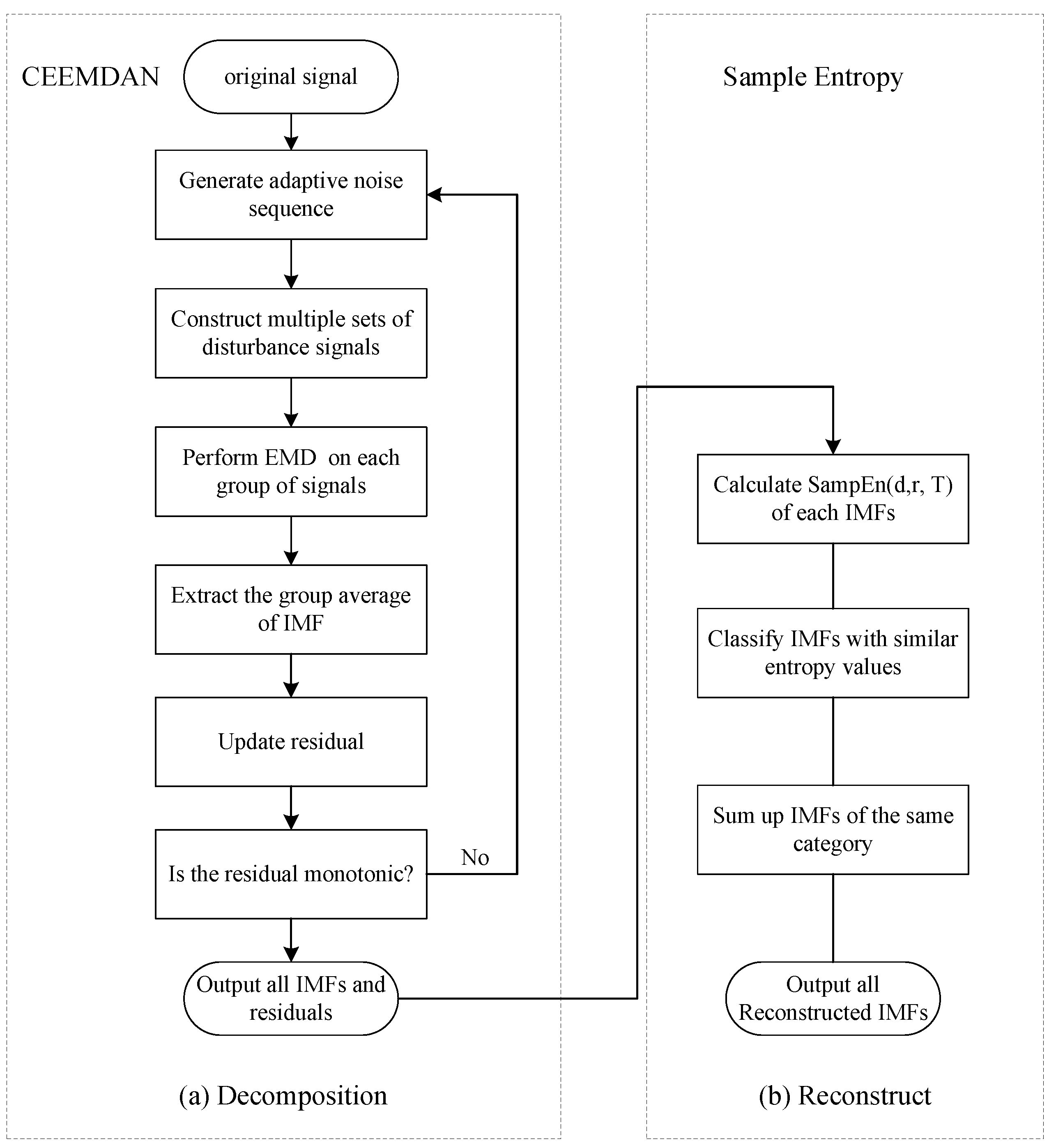
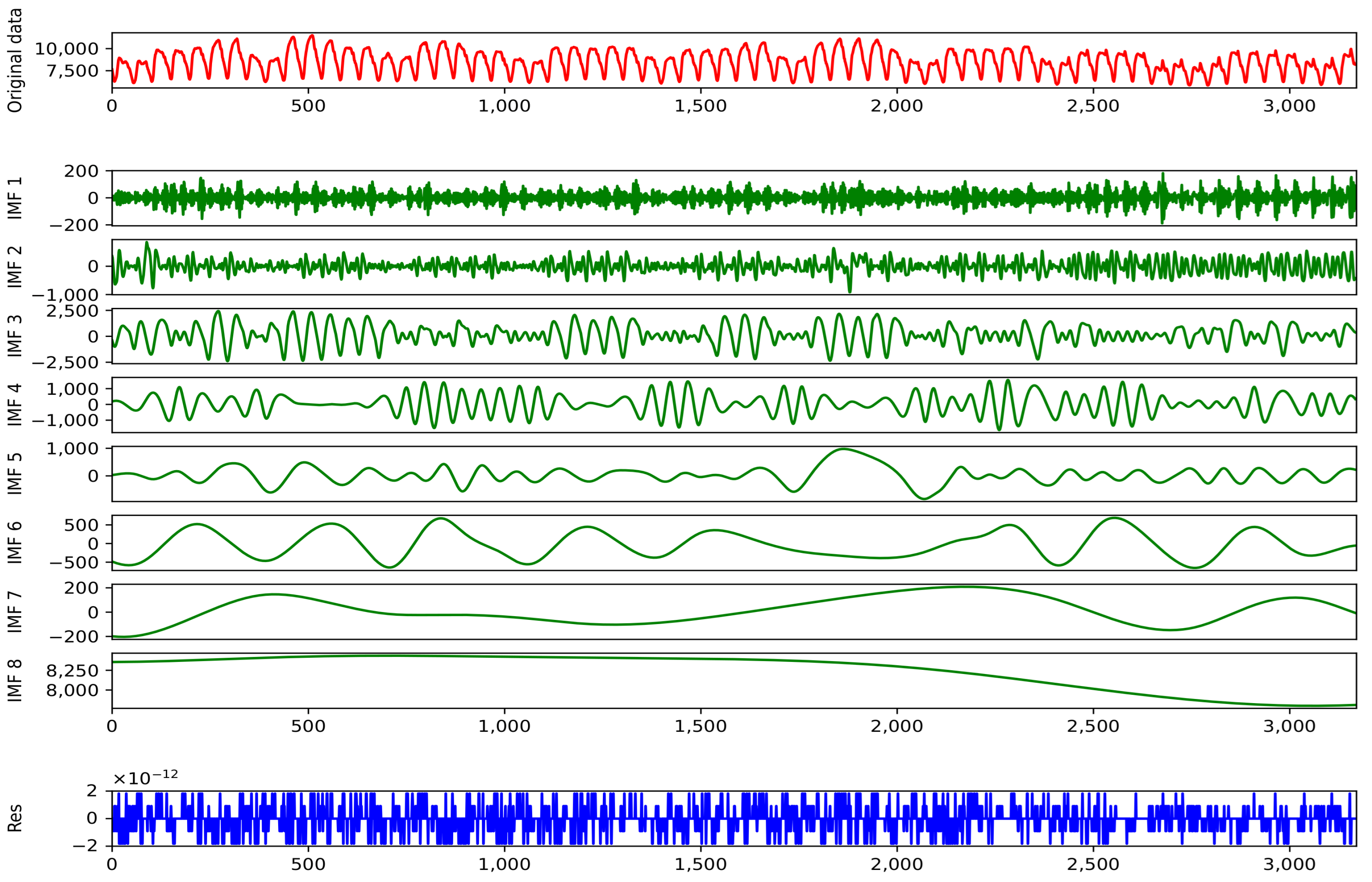
A flowchart of CEEMDAN decomposing power load data is visually captured in Figure 1a.

2.1.2. Sample Entropy

Independent forecasting of all IMFs derived from signal decomposition introduces dual computational challenges: exponential growth in processing overhead and neglect of inter-component interdependencies. Implementing correlation-aware component clustering and adaptive reprocessing achieves dual optimization: reducing computational latency through dimensional consolidation while enhancing feature saliency through homogeneous pattern amplification. This methodology leverages entropy-based metrics from information theory to stratify subcomponents by nonlinear dynamic similarity [69].

Sample entropy is proposed to measure the complexity of signal sequences based on approximate entropy [73]. Higher sample entropy indicates higher complexity of the sequence, and, on the contrary, the complexity of the sequence. The advantage of sample entropy over approximate entropy is that it is not compared to its data segment; the calculation results are independent of the length of the data and are more consistent. The steps for calculating the sample entropy are as follows:

Figure 1. Decomposition and reconstruction of data.

Figure 1. Decomposition and reconstruction of data.

For the given time sequence $X_d\left(1\right),\dots ,X_d(T-d+1)$, where d is the embedding dimension and T is the sample size, form the time series $X_d\left(t\right)=\{x\left(t\right),x(t+1),\dots ,x(t+d-1)\}$ for $1\le t\le T-d+1$. Then, the distance between $X_d\left(t\right)$ and $X_d\left(t^{\prime }\right)$ is defined as

$$\begin{array}{c}\hfill D[X_d\left(t\right),X_d\left(t^{\prime }\right)]=\underset{0\le s\le d-1}{max}\left(\right|x(t+s)-x(t^{\prime }+s)\left|\right),\end{array}$$

where $D[X_d\left(t\right),X_d\left(t^{\prime }\right)]$ is the infinite paradigm of difference between $X_d\left(t\right)$ and $X_d\left(t^{\prime }\right)$.

With a given tolerance r, $X_d\left(t\right)$ and $X_d\left(t^{\prime }\right)$ are r-similar if $D[X_d\left(t\right),X_d\left(t^{\prime }\right)]\le r$ for every s-th dimension. When $D[X_d\left(t\right),X_d\left(t^{\prime }\right)]\le r$, count the cardinality of $t^{\prime }$ not equal to t as $B_t$ for $t^{\prime }\in [1,T-d]$. Increased to the $d+1$-dimension, the number of summed $t^{\prime }$ under the same conditions can be calculated to obtain $A_t$, the count of vectors within a tolerance r for each t. Write this as

$$\begin{array}{c}{A}_t^d\left(r\right)={\displaystyle \frac{1}{T-d}}{\displaystyle \sum _{t=1}^{T-d}}{\displaystyle \frac{1}{T-d-1}}{A}_t\hfill \\ B_t^d\left(r\right)={\displaystyle \frac{1}{T-d}}{\displaystyle \sum _{t=1}^{T-d}}{\displaystyle \frac{1}{T-d-1}}{B}_t\hfill \end{array}$$

Then, the definition of sample entropy is given as the natural logarithm of the ratio of $A_i^d\left(r\right)$ to $B_i^d\left(r\right)$, which is specified as

$$\begin{array}{c}\hfill SE(d,r,T)=ln{B}_t^d\left(r\right)-ln{A}_t^d\left(r\right).\end{array}$$

(3)

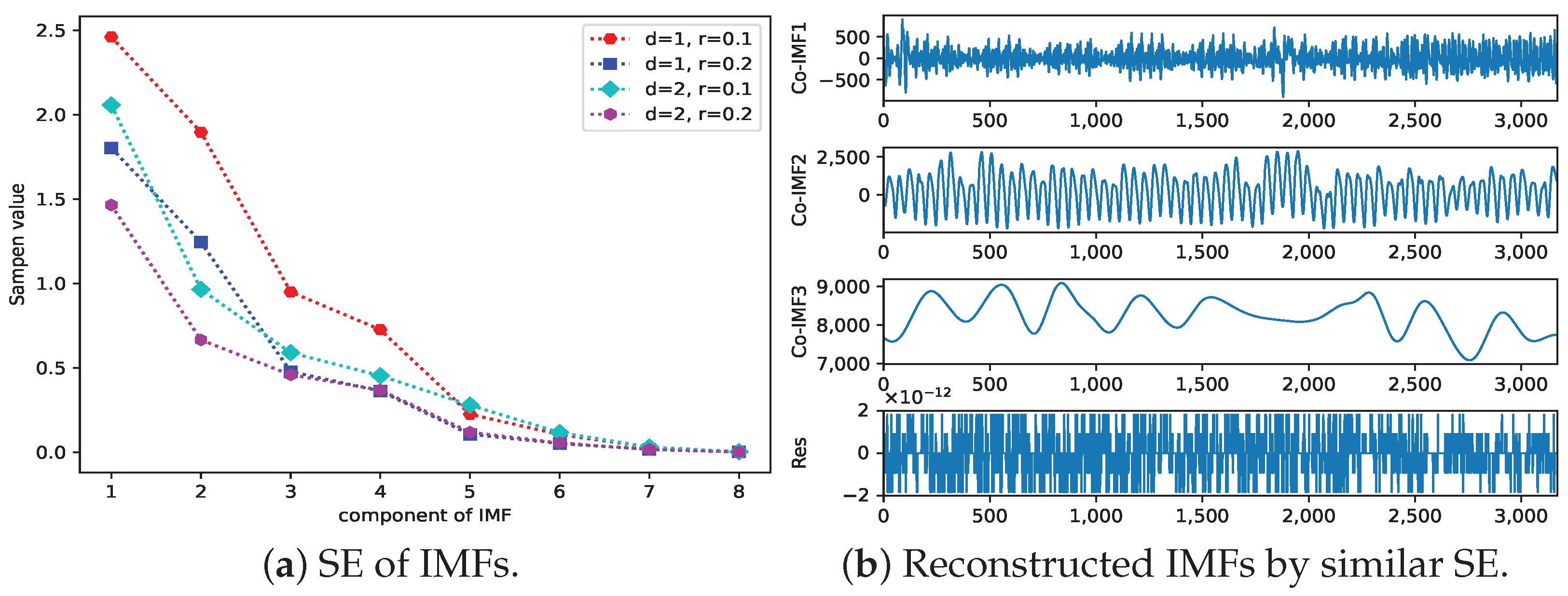
In practical applications, this typically sets d to 1 or 2, while generally r is determined as 10–$25\%$ of the standard deviation of the input data. Given the excessive number of subcomponents generated from the decomposition and the computational demands of data processing/training, we directly model and predict all subcomponents while employing sample entropy $SE(d,r,T)$ to assess their complexity. Subsequently, components exhibiting similar entropy values are systematically regrouped into four final categories for subsequent forecasting: high-frequency, medium-frequency, and low-frequency oscillations, and residual elements. The details of the reconstruction process are shown in Figure 1b.

2.2. SSA and Its Improvement

This section introduces the principle and specific implementation details of the ISSA proposed at the “optimization” level of hyperparameter selection in the hybrid models.

2.2.1. SSA

The sparrow search algorithm (SSA), a swarm intelligence metaheuristic emulating sparrow foraging dynamics through collective predator–prey interactions, demonstrates superior convergence velocity and solution precision compared to conventional optimization paradigms like particle swarm optimization (PSO) and Teaching–Learning-Based Optimization (TLBO). Its computational efficacy stems from hierarchical search strategies balancing global exploration and local exploitation, achieving enhanced computational efficiency in high-dimensional solution spaces [74].

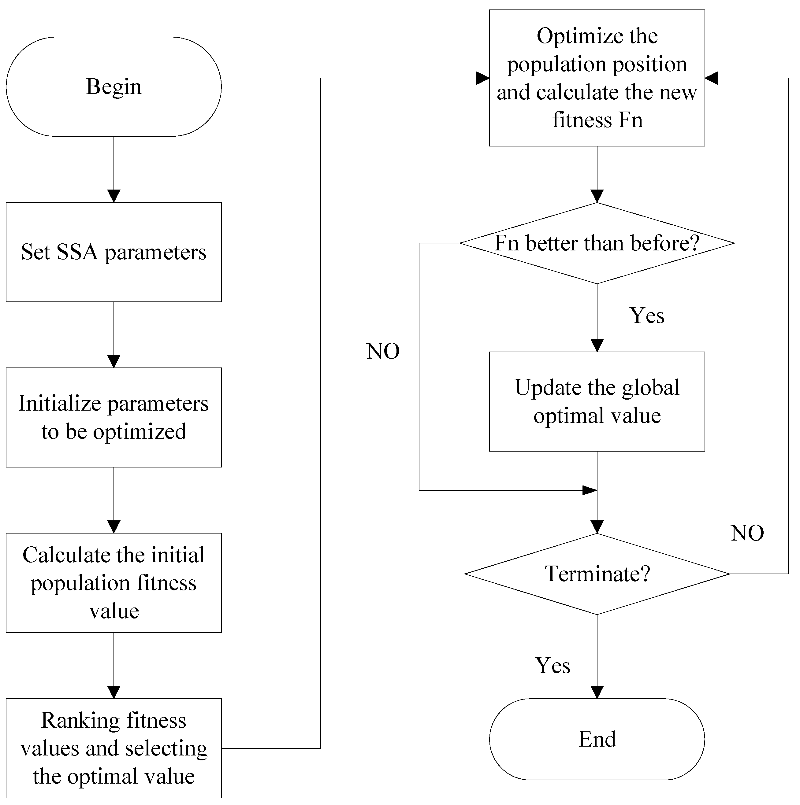
The SSA is inspired by the foraging behavior and anti-predation strategies of sparrows in nature. It simulates the interaction between producers (food-searching sparrows) and scroungers (followers) while incorporating a vigilance mechanism to avoid local optima. The flowchart of the SSA can be found in Figure 2. Its key principles include the following:

Figure 2. SSA chart.

Figure 2. SSA chart.

• Division of Roles: Sparrows are categorized into producers (explorers with high fitness) and scroungers (followers) to balance exploration and exploitation.
• Competition Mechanism: Scroungers compete with producers for food resources. If a scrounger fails, it relocates to avoid stagnation.
• Anti-Predation Behavior: Sparrows at the population’s edge move toward safer areas when threatened, while those in the center adjust positions randomly to maintain diversity.
• Adaptive Search: Producers perform broad exploration, while scroungers refine solutions locally, ensuring dynamic adaptation to the search space.

The SSA uses a random initialization of the population, which results in low diversity and quality of the initial population, which may affect the global search ability and final convergence accuracy. In the iterative update formula of the SSA, when an individual approaches the optimal solution, its position update formula will cause the individual to make small adjustments near the optimal solution instead of continuing to explore other regions. Therefore, the SSA is prone to becoming stuck in local optimal solutions, especially in complex optimization problems, and, in the later iteration stage, the convergence speed of the SSA is slow, making it difficult for the algorithm to further optimize.

2.2.2. ISSA

To overcome the blindness of the population initialization of the SSA, and to further boost both global search and local exploitation capabilities, an improved SSA is proposed. The improvements are as follows:

(1)

Implementation of a good point set for population initialization: Leveraging low-discrepancy sequence generation from good point set theory enhances initial population distribution in high-dimensional spaces. This geometrically driven initialization ensures spatial uniformity and diversity preservation, critically accelerating convergence kinetics while preventing premature solution stagnation.

(2)

Revision of discoverer dynamics via golden sine optimization: The golden sine (Gold-SA) mechanism is integrated into discoverer positional updating to maintain solution space dimensionality throughout iterations, effectively mitigating the local optima entrapment common in the conventional SSA.

(3)

Incorporation of Lévy flight for adaptive step size regulation: Lévy flight is used to improve the step size to increase the diversity of the population. The heavy-tailed distribution facilitates global optimum discovery through sporadic long-range jumps while maintaining intensive local search.

The basic steps of the ISSA are as follows:

Step 1: Initialize the population by applying the set of good points, which can be expressed as $P_n\left(i\right)=\left\{r_1{i}_1,r_2{i}_2,\dots ,r_n{i}_n\right\}$ for $i=1,\dots ,n$, where $\mathbf{r}=(r_1,\dots ,r_n)$ belongs to a unit cube in n-dimensional Euclidean space, the deviation $\phi$ of $P_n\left(i\right)$ satisfies $\phi \left(n\right)=C(r,ϵ)n^{-1+ϵ}$, $C(r,ϵ)n^{-1+ϵ}$ is a constant related only to r and $ϵ$, and $P_n\left(i\right)$ is said to be the good point set. Let $r_j=2cos\left(2\pi j/p\right)$ for $1\le j\le n$, and $\mathbf{r}$ is the set of good points. Map $P_n$ to the search space as follows: $X_i^j=a_j+P_n\left(i\right)(b_j-a_j)$, where $a_j$ and $b_j$ denote the lower and upper limits of the current dimension, respectively.

Step 2: The proportion of discoverers in the population is denoted as PD and is generally taken to be between $10\%$ and $20\%$. The formula for updating the location of discoverers is written as

$$\begin{array}{c}{X}_{i,j}^{t+1}=\left\{\begin{array}{cc}GS(X_{i,j}^t,X_P^t),\hfill & R_2<ST,\hfill \\ X_{i,j}^t+Q·L,\hfill & R_2\ge ST,\hfill \end{array}\right.\hfill \end{array}$$

(4)

where $X_{i,j}^t$ denotes the position of the i-th individual in the j-th dimension at the current number of iterations, $GS(X_{i,j}^t,X_P^t)\triangleq X_{i,j}^t·|sin\left(r_1\right)|-r_2·sin\left(r_1\right)·|c_1{X}_P^t-c_2{X}_{i,j}^t|$ represents the golden sine strategy, $r_1$ and $r_2$ are random numbers taking the values $[0,2\pi ]$ and $[0,\pi ]$, respectively, and $X_P^t$ is the position of the current optimal individual. $c_1$ and $c_2$ are calculated using the equations as $c_1=a·\left(1-\tau \right)+b·\tau$ and $c_2=a·\tau +b·\left(1-\tau \right)$, where a and b represent the search intervals for each search, and $\tau =(\sqrt{5}-1)/2$ is the golden ratio, which takes the value of approximately 0.618033.

Step 3: Update the position of the followers by

$$\begin{array}{c}\hfill X_{i,j}^{t+1}=\left\{\begin{array}{cc}Q·exp\left((X_{\mathrm{worst}}^t-X_{i,j}^t)/i^2\right),\hfill & i>{\displaystyle \frac{N}{2}},\hfill \\ X_p^{t+1}+|X_{i,j}^t-X_p^{t+1}|·A^{+}·L,\hfill & i\le {\displaystyle \frac{N}{2}},\hfill \end{array}\right.\end{array}$$

(5)

where $x_p^{t+1}$ denotes the optimal location where the discoverer is located in generation $t+1$, $X_{worst}^t$ denotes the worst position occupied in generation t, A denotes a matrix of dimension $1\times d$ with elements of 1 or $-1$, and $A^{+}=A^T{\left(A{A}^T\right)}^{-1}$ is the transformation matrix of A. It indicates that the i-th follower is less adapted when $i>n/2$, and the sparrow needs to fly to a farther location to forage for food. It also indicates that the i-th follower is more adapted when $i\le n/2$, and the sparrow does not need to make a wide range of transfers.

Vigilantes are generally adopted as comprising between $10\%$ and $20\%$ of the population, and their positions are updated using the following formula:

$$\begin{array}{c}\hfill {\mathbf{X}}_{i,j}^{t+1}=\left\{\begin{array}{cc}LFS({\mathbf{X}}_{i,j}^t,{\mathbf{X}}_{\mathrm{best}}^t),\hfill & \hfill f_i>f_g,\\ {\mathbf{X}}_{i,j}^t+k·{\displaystyle \frac{|{\mathbf{X}}_{i,j}^t-{\mathbf{X}}_{\mathrm{worst}}^t|}{|f_i-f_w|+\epsilon }},\hfill & \hfill f_i=f_g,\end{array}\right.\end{array}$$

(6)

where $LFS({\mathbf{X}}_{i,j}^t,{\mathbf{X}}_{\mathrm{best}}^t)\triangleq Levy\left(d\right)·{\mathbf{X}}_{\mathrm{best}}^t+\beta ·|{\mathbf{X}}_{i,j}^t-Levy\left(d\right)·{\mathbf{X}}_{\mathrm{best}}^t|$ is the Lévy flight strategy with Lévy flight path $Levy\left(d\right)=r_1/|r_2{|}^{1/\beta }$, d is the dimension, $s_1\sim N(0,1)$, $s_2\sim N(0,{\sigma }_v^2)$ with

$$\begin{array}{c}\hfill {\sigma }_v={\left\{{\displaystyle \frac{\Gamma \left(1+\beta \right)sin\left(\pi \beta /2\right)}{\Gamma \left[\left(1+\beta \right)/2\right]2^{\left(\beta -1\right)/2}\beta }}\right\}}^{1/\beta },\end{array}$$

$\Gamma$ is the gamma function, and $\beta \in (0,2)$ is a constant with a constant value of 1.5.

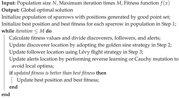
The flowchart of the ISSA will be delayed in the introduction of CEEMDAN-ISSA-CNN-BiLSTM in Section 2.4.2. To specifically demonstrate the algorithm process of the ISSA, we provide the pseudocode of the ISSA in Algorithm 1. It can be seen that the time complexity of the ISSA mainly consists of the initialization phase and the iterative update phase, with an overall time complexity of $O(M\times n\times d)$ and space complexity of $O(n\times d)$, where M is the maximum of the iteration. The ISSA significantly improves the convergence speed, global search capability, and robustness of the SSA through the initialization of the optimal cluster, golden sine strategy, and Lévy flight strategy. Under the premise of controllable time complexity, its improvement strategy effectively solves the problems of the original algorithm: tendency to become stuck in local optima and low search efficiency in the later stage. Therefore, this study integrates the ISSA into the hybrid model to select the hyperparameters for STLF.

Algorithm 1: ISSA

2.3. CNN-BiLSTM

The CNN-BiLSTM model adopts a parallel structure which can simultaneously process different aspects of information and comprehensively understand complex patterns in data [43,44,75]. This section will introduce the CNN, BiLSTM, and the hybrid of the CNN and BiLSTM (i.e., CNN-BiLSTM), respectively.

2.3.1. CNN

A CNN is a deep neural network with a convolutional structure and is one of the most commonly used models in recent years. A CNN is mainly used for extracting data features and classification [76] with high robustness and fast computational efficiency. The framework of a CNN consists of input, convolutional, pooling, fully connected, and output layers. The convolutional layer uses convolution kernels to perform convolution operations on input data and extract local features. The pooling layer can reduce the spatial dimension of feature maps, thereby enhancing the robustness and generalization ability. The fully connected layer is used for classification or regression, etc. The structure of a CNN is schematically detailed in Figure 3.

This study chooses a CNN because time series data can be smoothly input into convolutional neural networks. The model can directly learn temporal features, reduce data complexity, mine internal relationships of data, and eliminate noise and unstable factors.

2.3.2. BiLSTM

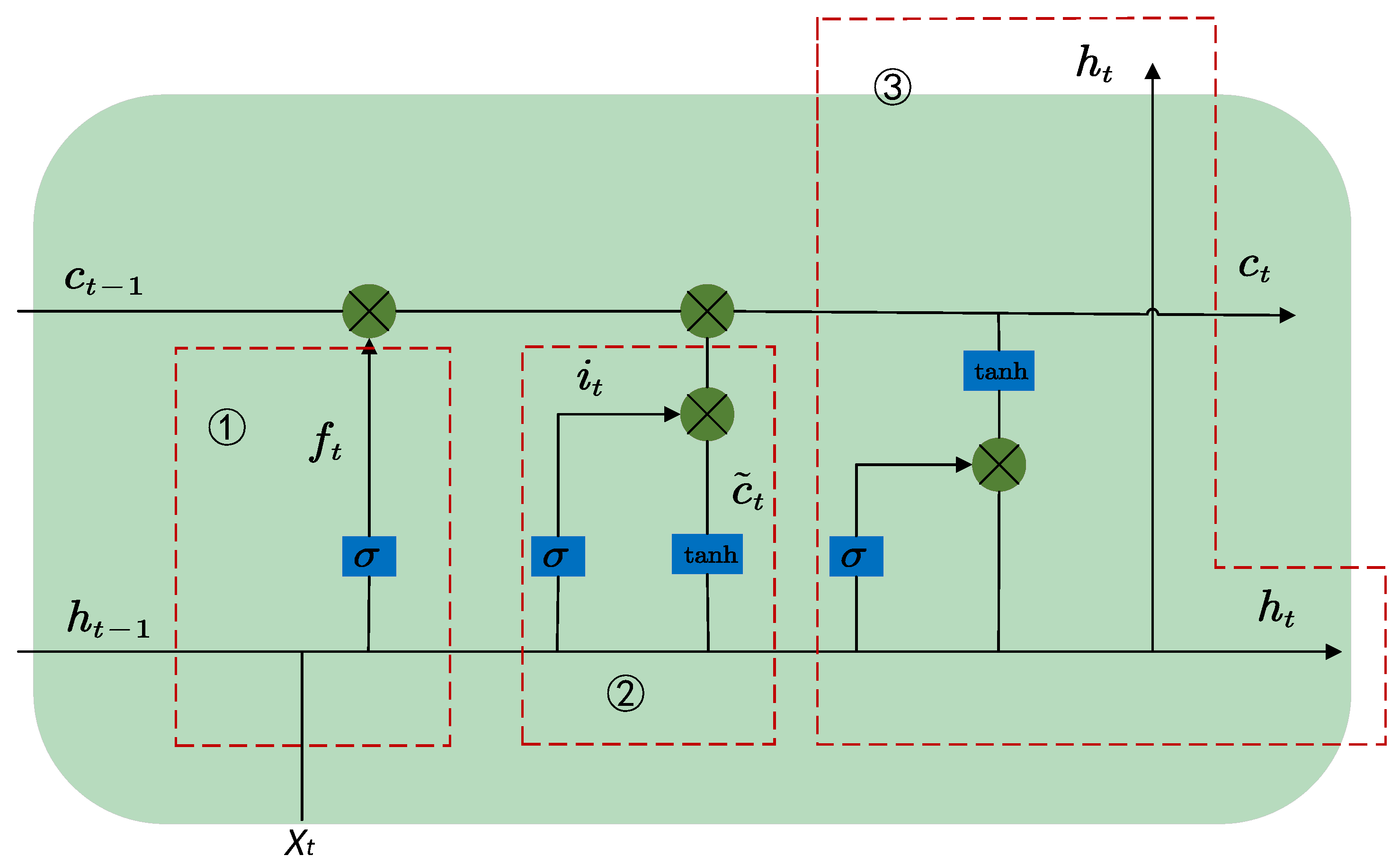
Long short-term memory (LSTM) networks, introduced by Hochreiter and Schmidhuber [27] as a specialized recurrent architecture, fundamentally extend conventional RNN capabilities through three innovative gating units: the input, forget, and output gates. These gates collectively facilitate the enhanced processing of extended temporal sequences by implementing selective memory retention mechanisms—a critical advancement enabling superior long-term dependency modeling compared to basic RNN structures. The input gate regulates information assimilation, the forget gate controls historical memory retention, and the output gate manages hidden state propagation. This tripartite gating system equips LSTM with persistent memory capabilities through controlled cell state transitions, overcoming traditional RNN limitations in capturing distant temporal relationships. The detailed architectural configuration is shown in Figure 4.

The forget gate is used to decide what information to remove in the cell state, and its structure is shown in the dashed box where ➀ is located in Figure 4. The input and output gate can control the flow of information in and out, and the structure is shown in the dashed box where ➁ and ➂ are located in Figure 4. The three gates can address the issues of gradient vanishing or exploding in RNNs and enable the LSTM to better capture long-term dependencies. Equations (7)–(11) represent a single LSTM. Specifically, LSTM unit status in Figure 4 can be represented by

$$\begin{array}{cc}\hfill f_t& =\sigma \left(W_f·\left[h_{t-1},x_t\right]+b_f\right),\hfill \end{array}$$

(7)

$$\begin{array}{cc}\hfill i_t& =\sigma \left(W_i·\left[h_{t-1},x_t\right]+b_i\right),\hfill \end{array}$$

(8)

$$\begin{array}{cc}\hfill o_t& =\sigma \left(W_f·\left[h_{t-1},x_t\right]+b_o\right).\hfill \end{array}$$

(9)

Candidate memories are calculated as

$$\begin{array}{cc}\hfill & {\tilde{C}}_t=tanh\left(W_c·\left[h_{t-1},x_t\right]+b_{\mathrm{c}}\right),\hfill \end{array}$$

(10)

$$\begin{array}{cc}\hfill & C_t=f_t\ast C_{t-1}+i_t\ast {\tilde{C}}_t,\hfill \end{array}$$

(11)

where $f_t$, $i_t$, and $o_t$ indicate the value of forgetting, input, and output gates at the current moment, and $h_{t-1}$ and $x_t$ denote the hidden layer status of the preceding moment and the current moment input value. $W_f$, $W_i$, and $W_o$ denote the weight matrix, $b_f$, $b_i$, and $b_o$ denote bias vectors, and $\sigma$ and tanh denote the sigmoid and tanh activation layer, respectively, which is compressed in the range of $[0,1]$. The formula is given as

$$\begin{array}{c}\hfill \sigma \left(x\right)={\displaystyle \frac{1}{1+exp(-x)}},tanh\left(x\right)={\displaystyle \frac{exp\left(x\right)-exp(-x)}{exp\left(x\right)+exp(-x)}}.\end{array}$$

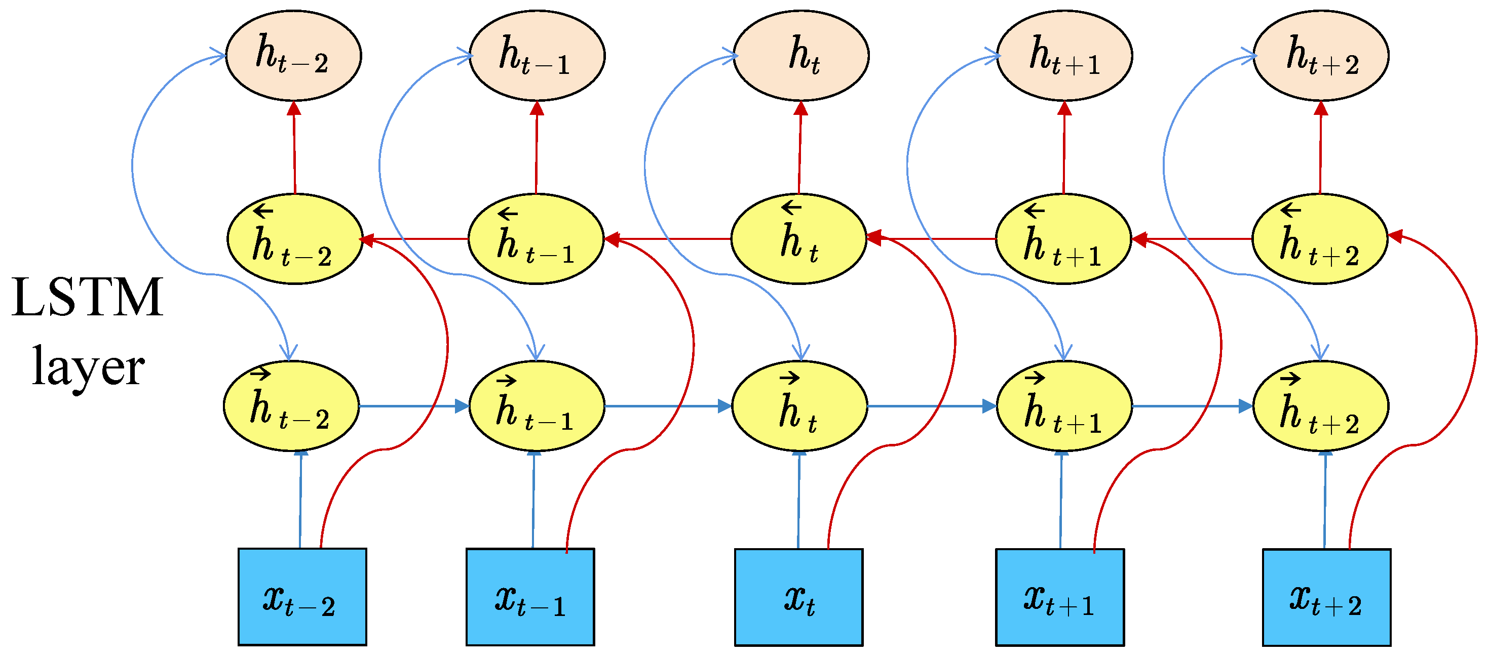
BiLSTM works by linking two LSTM networks that process sequences in opposite directions, enabling the capture of both past and future information in the same output, and Figure 5 shows the structure. The forward LSTM scans from the beginning to the end of the input sequence, and the reverse LSTM scans from the end to the beginning. The advantage of BiLSTM is that it can consider both historical and future information and better capture relevant features in the sequence, which improves the ability to model sequence data. The formula can be expressed as

$$\begin{array}{c}\hfill {\overrightarrow{h}}_t=LSTM(x_t,{\overrightarrow{h}}_{t-1}),{\overleftarrow{h}}_t=LSTM(x_t,{\overleftarrow{h}}_{t-1}),\end{array}$$

where ${\overrightarrow{h}}_t$ and ${\overleftarrow{h}}_t$ represent the hidden states of the forward and reverse LSTM at the t-th moment, respectively, $x_t$ is the current input, and the output of the BiLSTM is about to splice ${\overrightarrow{h}}_t$ and ${\overleftarrow{h}}_t$.

Figure 5. BiLSTM framework chart.

Figure 5. BiLSTM framework chart.

2.3.3. CNN-BiLSTM

The CNN-BiLSTM architecture integrates sequential convolutional processing with bidirectional temporal modeling through five core components: an input module, convolutional-pooling hierarchy, bidirectional LSTM layers, fully connected integration, and task-specific output. The input module serves as the data ingestion interface for raw sequential inputs. Subsequent convolutional layers perform hierarchical feature abstraction through kernel-based spatial filtering, with pooling operations enhancing translational invariance. These processed features feed into bidirectional LSTM layers that model contextual dependencies through forward–backward hidden state propagation, effectively capturing both precedent and subsequent temporal patterns. The fully connected layer executes feature aggregation via nonlinear transformation of concatenated BiLSTM outputs, while the terminal layer employs task-specific activation functions (e.g., softmax for classification, linear for regression) to generate predictions. This architecture’s synergistic combination of spatial feature extraction and contextual sequence modeling establishes it as the optimal predictive engine within our hybrid framework.

2.4. Improved Hybrid Models for STLF

This section will integrate the ISSA and CEEMDAN into the hybrid model one by one to evaluate the improvement of the model. Section 2.4.1 proposes ISSA-CNN-BiLSTM, combining the ISSA and CNN-BiLSTM. Section 2.4.2 builds CEEMDAN-ISSA-CNN-BiLSTM by using CEEMDAN and sample entropy to decompose and reconstruct the original data for the input of the ISSA-CNN-BiLSTM.

2.4.1. ISSA-CNN-BiLSTM for STLF

In ISSA-CNN-BiLSTM, we use the ISSA to optimize four parameters in CNN-BiLSTM, including the learning rate ($\alpha$), the number of neurons in the first and second convolutional layers ($fc$, $sc$), and the number of BiLSTM neurons (h). Thus, the model can be written as

$$\begin{array}{c}\hfill \left\{\begin{array}{c}\mathrm{fitness}={\displaystyle \frac{100\%}{T}}\sum _{t=1}^T\left|{\displaystyle \frac{{\widehat{y}}_t-y_t}{y_t}}\right|,\hfill \\ {\widehat{y}}_t=f_{CNN-BiLSTM}(\mathbf{y},\alpha ,fc,sc,h),\hfill \end{array}\right.\end{array}$$

(12)

where the fitness of the optimization in the ISSA is the mean absolute percentage error (MAPE) of the prediction results calculated by the mapping $f_{CNN-BiLSTM}$ of CNN-BiLSTM, and ${\widehat{y}}_t$ and $y_t$ denote the predicted values and the true value, respectively, of the time series set for the training model. ${\alpha }_{min}\le \alpha \le {\alpha }_{max}$ with the upper bound ${\alpha }_{max}$ and lower bound ${\alpha }_{min}$ of $\alpha$, ${fc}_{min}\le fc\le {fc}_{max}$, ${sc}_{min}\le sc\le {sc}_{max}$, and $h_{min}\le h\le h_{max}$, and have bounds similar to $\alpha$.

The steps of the ISSA to optimize CNN-BiLSTM are as follows:

Step 1: Set the ISSA optimization parameters, including population size, number of iterations, and upper and lower limits of parameters to be optimized, and use the good point set to determine the initial population size.

Step 2: Use CNN-BiLSTM for training data to calculate and rank the fitness values, and denote the minimum fitness value as ${fitness}_{new}\left(j\right)$.

Step 3: Use good sets to update the population position and calculate the fitness value. Compare ${fitness}_{new}\left(j\right)$ with the fitness value of the previous iteration. If the fitness value decreases, then update the global optimal parameters.

Step 4: Determine whether to stop the calculation. If not, continue to update the position of the sparrow using Equations (4)–(6); otherwise, stop the optimization.

Step 5: Obtain the final model with the optimized parameters in ISSA-CNN-BiLSTM.

The ISSA dynamically optimizes CNN-BiLSTM hyperparameters—including learning rate and hidden layer dimensionality—through iterative population-based optimization, employing the mean squared error (MSE) as the fitness metric. This automated approach reduces computational overhead from manual hyperparameter configuration by 62–78% compared to grid search methodologies. The metaheuristic global exploration of the ISSA synergistically integrates with the local feature extraction and bidirectional temporal modeling capabilities of CNN-BiLSTM, achieving dual enhancement: more prediction accuracy through optimized network architectures and faster convergence via adaptive learning rate scheduling.

2.4.2. CEEMDAN-ISSA-CNN-BiLSTM for STLF

This section proposes CEEMDAN-ISSA-CNN-BiLSTM combining signal decomposition technology, deep learning, and optimization algorithms. The flowchart of CEEMDAN-ISSA-CNN-BiLSTM is illustrated in Figure 6.

The specific steps of CEEMDAN-ISSA-CNN-BiLSTM can be represented as follows:

Step 1: Divide the original power load data into training and testing sets.

Step 2: Data preprocessing:

• Use CEEMDAN to decompose data into IMFs and a residual component.
• Calculate the sample entropy of each IMF and reorganize the K IMFs into four terms: high frequency, medium frequency, low frequency, and residual component.
• Set the sliding window and step size, construct the input matrix, and normalize it.

Step 3: Determine hyperparameters required for optimization in ISSA-CNN-BiLSTM.

Step 4: Train ISSA-CNN-BiLSTM sub-models:

• Use the ISSA in Section 2.2.2 to optimize the hyperparameters in the K sub-models.
• Import the input matrix into the network and obtain the best parameters.

Step 5: Input the test matrix into the network corresponding to the optimization parameters to obtain the predictions using each sub-model.

Step 6: Integrate the predictions of each sub-model to calculate the final prediction.

Figure 6. Flowchart of CEEMDAN-ISSA-CNN-BiLSTM.

Figure 6. Flowchart of CEEMDAN-ISSA-CNN-BiLSTM.

To comprehensively compare CEEMDAN-ISSA-CNN-BiLSTM with other popular state-of-the-art models, we summarize the strengths and weaknesses of these models in

Table 1. Comparison of CEEMDAN-ISSA-CNN-BiLSTM with other popular state-of-the-art models.

Model	Advantage	Disadvantage	Scenarios
CEEMDAN-ISSA-CNN-BiLSTM	Combining CEEMDAN to reduce data non-stationarity and improve prediction accuracy	High computational complexity	High precision requirements and complex temporal fluctuation scenarios
	ISSA optimization enhances the efficiency of hyperparameter search	Long training time and relies on a large number of data
	CNN extracts spatial features, BiLSTM captures bidirectional temporal dependencies
CEEMDAN-IWOA-LSTM [77]	CEEMDAN optimizes input features to reduce noise interference	Using only unidirectional LSTM has limited temporal modeling capabilities	Medium complexity, univariate time series prediction
	The IWOA algorithm efficiently optimizes LSTM parameters with small errors	Unfused spatial feature extraction module
CEEMDAN-TCN-LSTM [78]	TCN has strong parallel computing capability and fast training speed	TCN is sensitive to local features and may ignore global patterns	Large-scale data and high real-time requirements for scenarios
	LSTM supplements long-term dependency modeling	Unintegrated signal decomposition method
Transformer-Based [79]	Self-attention mechanism captures long-range dependencies	Extremely high demand for computing resources	Ultra-long-sequence, multivariate correlation scenario
	No need for manual feature engineering	Strict requirements for data volume, poor performance in small sample sizes
PSO-A2C-Lnet [80]	PSO hyperparameters to avoid overfitting	The model structure is complex and the deployment difficulty is high	Multi-source heterogeneous data and strong spatiotemporal correlation
	Multi-head attention enhances feature importance learning	Multi-stage training is required and time consuming

. CEEMDAN requires multiple iterations of computation, with a complexity in terms of data length. The combination of a CNN and BiLSTM results in a large number of parameters. The ISSA optimization requires multiple fitness assessments, and the total complexity is significantly higher than that of a single model. The complexity of traditional LSTM is in time steps, in hidden layer dimensions [40], while CEEMDAN-ISSA-CNN-BiLSTM may increase its complexity by 2–3 times due to the stacking of multiple components.

CEEMDAN-ISSA-CNN-BiLSTM significantly improves prediction accuracy through signal decomposition and a hybrid model structure, but at the cost of sacrificing computational efficiency. CEEMDAN decomposition layers can be simplified (such as reducing modal components) or parameter-sharing strategies adopted. GPU parallelization is utilized for CNN and BiLSTM computation to reduce training time. CEEMDAN-ISSA-CNN-BiLSTM performs excellently in complex temporal prediction, but its high computational cost needs to be balanced in practical applications. In the future, efficiency can be further improved through model compression (such as knowledge distillation) and adaptive decomposition algorithms (dynamic CEEMDAN).

The proposed CEEMDAN-ISSA-CNN-BiLSTM systematically solves the three major challenges—the non-stationarity of load power data, low efficiency of hyperparameters, and insufficient feature recognization in the STLF field—through the three-level “decomposition–optimization–prediction” innovation. CEEMDAN and sample entropy can decompose and reconstruct the data to improve the SNR. The ISSA can significantly improve the convergence speed, global search capability, and robustness of the SSA for the selection of hyperparameters in deep learning models through the initialization of the optimal cluster, golden sine strategy, and Lévy flight strategy. CNN-BiLSTM calculates good evaluation index values, and BiLSTM can better discover the short-term and long-term correlations of power load data. Therefore, according to the optimum at the three levels of “decomposition–optimization–prediction”, CEEMDAN-ISSA-CNN-BiLSTM theoretically performs better than the other alternative models.

3. Case Study and Analysis

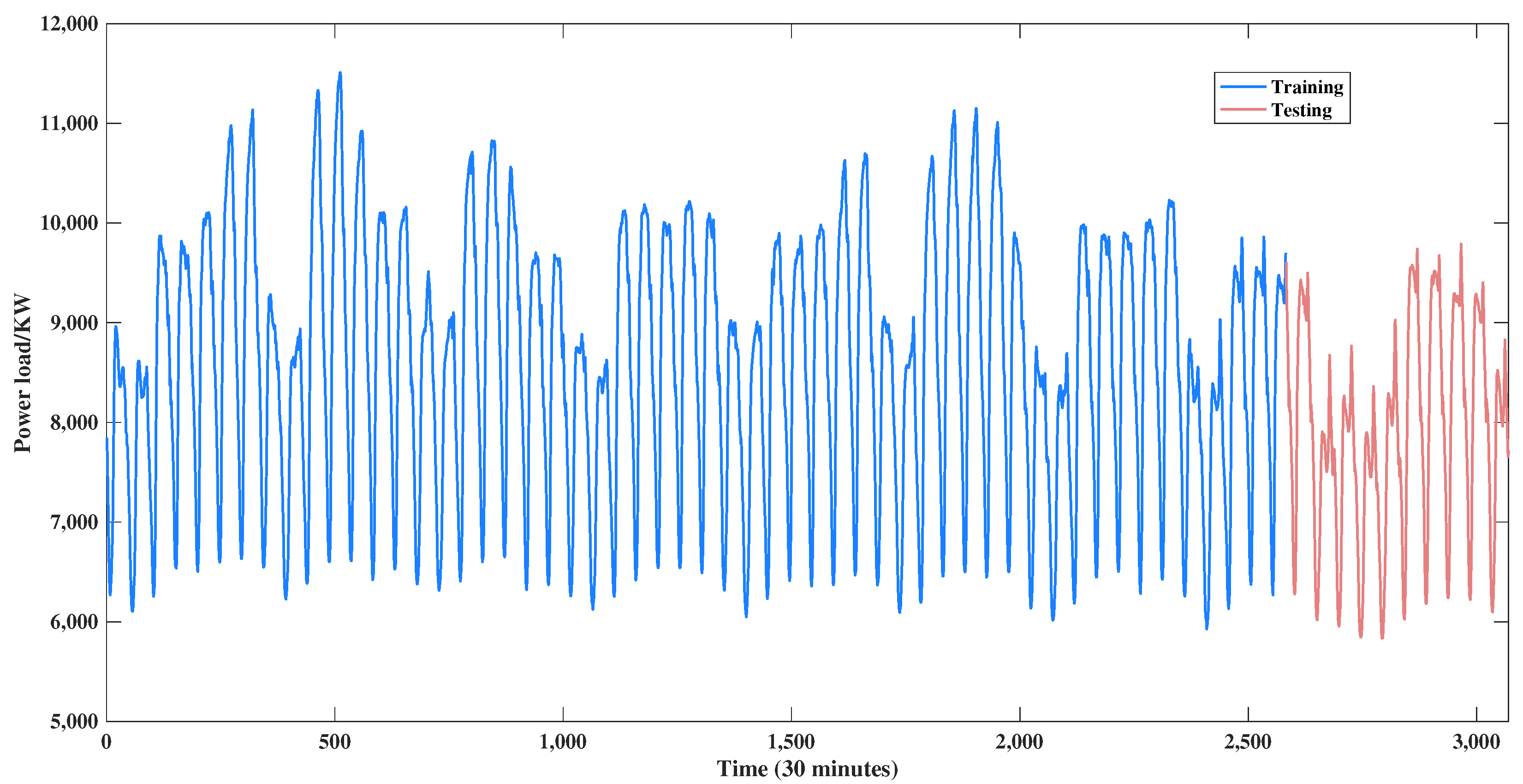
In this study, we use the load data of an area in Australia from 14 February 2009 to 20 April 2009 for STLF by the proposed model. The data were recorded at 30 min intervals, and 48 points were collected every day, making a total of 3168 load data.

3.1. Data Sources and Processing

We partition the data into the training set, validation set, and test set. Normalization transforms data with different scales into a uniform range of values and decomposes and reconstructs the data using CEEMDAN and sample entropy.

3.1.1. Data Partitioning

The data are divided according to the ratio of 4:1, where the first $80\%$ of the data are used as the training set, and the last $20\%$ are used as the validation and test sets. This partitioning method is common in time series prediction tasks, ensuring that the model is trained and evaluated on data from different periods, thereby improving the generalization ability of the model [81]. In addition, traditional cross-validation methods, such as K-fold cross-validation, typically assume that the samples are independent and identically distributed, but this assumption does not hold in time series data. If future data are included in the training set and historical data are included in the validation set, it may cause the model to use future information to predict historical results, resulting in bias [82]. Therefore, this study adopts sliding window technology, similar to Liu et al. [83], with a window width of 48, and uses data from the past 24 h to predict the next moment to avoid overfitting of the models. Sliding window technology can effectively improve the accuracy of load forecasting and reduce losses in the power system by capturing short-term dependencies and long-term trends [84]. Figure 7 shows the visualization of the original datasets.

3.1.2. Data Normalization

From Figure 7, it can be seen that the range of the original data varies greatly and has characteristics such as periodicity, volatility, and randomness. This will lead to some parameters being updated too quickly or too slowly during the model training process, thereby affecting the convergence speed of the model. Data normalization transforms data with different scales into a uniform range of values, typically mapping the data between 0 and 1, which helps the model converge faster. Normalizing the data will not shape the original distribution, but will make the data easier to compare and process. Normalization can also improve the efficiency and accuracy of some machine learning algorithms. In addition, we use the minimum–maximum scaling method to process the data as follows:

$$\begin{array}{c}\hfill x_{norm}={\displaystyle \frac{x-x_{min}}{x_{max}-x_{min}}},\end{array}$$

(13)

where x is the original data, and $x_{min}$ and $x_{max}$ are the maximum and minimum of the data.

3.1.3. Data Decomposition and Reconstruction

Figure 7 shows that the load data exhibit strong volatility and nonlinear characteristics. Therefore, it is necessary to use CEEMDAN to denoise the load data. The 3168 load data are decomposed by the CEEMDAN algorithm into eight IMFs and residuals. The red line in Figure 8 shows the original sequence and the blue line shows the result after CEEMDAN.

The calculation of sample entropy mainly involves two parameters: the model dimension (d), which is used to calculate the window length of the sample entropy, and the sequence, which can be divided into $n-d+1$ sequences. Usually, d takes 1 or 2. When the value of r is too small, it is possible that the statistical properties of the system cannot be estimated ideally. Usually, the value of r is between $0.1·std$ and $0.25·std$, and $std$ denotes the standard deviation of the original sequence. To balance the accuracy and computational efficiency of information capture, we take embedding dimension values of 1 and 2 and similarity thresholds of 0.1 and 0.2. Figure 9a shows the sample entropy of each IMF obtained by CEEMDAN. The horizontal axis represents the component of the IMF, and the vertical axis represents the sample entropy value. IMF1, IMF, and IMF3 have high complexity, and, in power load forecasting, high-frequency noise components usually have high sample entropy values.

In practical application, it will increase the time and memory requirement of computation substantially if all IMFs are introduced into the model, and there is a possibility of an overfitting phenomenon. Therefore, to reduce the computation volume and time while guaranteeing the prediction accuracy, in this paper, the sequence is reorganized into four intrinsic IMFs based on the sample entropy of the eight IMFs to obtain better predictions: high frequency, medium frequency, low frequency, and residuals. The reorganized sequence is shown in Figure 9b. The sample entropy values between the IMF1 and IMF2 are close to each other, indicating that the probability of these two components generating new patterns is roughly the same and the two components are superimposed to form a new subsequence as IMF1. The difference in sample entropy between IMF3, IMF4, and IMF5 is small, so they are reorganized into mid-frequency data as IMF2. The sample entropy of IMF6, IMF7, and IMF8 is the same, so they are reorganized into low-frequency data as IMF3.

3.2. Performance Criteria

To measure the accuracy and predictive ability of the prediction model, the commonly used root mean square error (RMSE), mean absolute error (MAE), and mean absolute percentage error (MAPE) are chosen to evaluate the model, where the criteria can be expressed by

$$\begin{array}{c}\hfill \begin{array}{c}\mathrm{RMSE}=\sqrt{{\displaystyle \frac{1}{T}}{\displaystyle \sum _{t=1}^T}{\left({\widehat{y}}_t-y_t\right)}^2},\hfill \\ \mathrm{MAE}={\displaystyle \frac{1}{T}}{\displaystyle \sum _{t=1}^T}\left|{\widehat{y}}_t-y_t\right|,\hfill \\ \mathrm{MAPE}={\displaystyle \frac{100\%}{T}}{\displaystyle \sum _{t=1}^T}\left|{\displaystyle \frac{{\widehat{y}}_t-y_t}{y_t}}\right|,\hfill \end{array}\end{array}$$

where ${\widehat{y}}_t$ and $y_t$ denote the t-th predicted value and true value, and n indicates the data size.

3.3. Data Sources and Processing

When designing the CNN-BiLSTM model, it is necessary to set some hyperparameters to control the architecture and training process of the network, and the setting of hyperparameters can greatly affect the performance and generalization ability of the model. After several experiments, the optimizer of CNN-BiLSTM is chosen to be RMSprop. BiLSTM and CNN models use sigmoid and ReLU activation functions, respectively. The CNN chooses two layers, and the number of filters in the first layer and the second layer is 32 and 64. The number of layers of BiLSTM is set as 1 and the number of neurons in the hidden layer of BiLSTM as 30.

The ISSA is used to optimize the initial learning rate, the number of nodes in the first and second convolutional layers, and the number of nodes in the BiLSTM. To compare the effectiveness of the ISSA-optimized models, SSA-optimized models are also introduced in this paper. All the settings of the parameters of the SSA and ISSA in the process of optimizing the CNN-BiLSTM parameters are shown in

Table 2. The parameters of the SSA and ISSA.

Algorithm	Parameter	Settings
	Population size	10
	The number of iterations	10
SSA	Proportion of finders	0.2
	Warning value	0.8
	lb	$[0.0001,10,10,10]$
	ub	$[0.01,100,100,100]$
	Population size	10
	The number of iterations	10
ISSA	Proportion of finders	0.2
	Warning value	0.8
	lb	$[0.0001,10,10,10]$
	ub	$[0.01,100,100,100]$

.

The hyperparameters optimized for the CEEMDAN-ISSA-CNN-BiLSTM model are detailed in

Table 3. Details of hyperparameter tuning.

Hyperparameter	Options	Optimization	Justification
Learning Rate	[0.0001, 0.01]	$1.2304\times {10}^{-4}$	ISSA selects the optimum within bounds while balancing convergence speed and stability.
CNN Layers	Layers	2 (Fixed)	Predefined to balance feature extraction and computational efficiency.
CNN Filters	Layer 1: [10, 100] Layer 2: [10, 100]	Layer 1: 32 Layer 2: 64	Optimized by ISSA to capture spatial patterns; higher filters in deeper layers enhance feature abstraction.
BiLSTM Units	[10, 100]	30 units	ISSA optimized to balance temporal modeling capacity and overfitting risks.
Activation Functions	CNN: ReLU BiLSTM: Sigmoid	Fixed	ReLU avoids vanishing gradients in CNN; sigmoid in BiLSTM gates regulates information flow.

. These parameters are selected based on empirical experimentation and optimization via the ISSA: (1) Learning rate: Optimized via the ISSA to avoid manual tuning bias. The range [0.0001, 0.01] is chosen empirically to ensure stable convergence; (2) CNN architecture: Two convolutional layers with 32 and 64 filters are selected to balance feature extraction depth and computational cost; (3) BiLSTM units: 30 units optimized by the ISSA to capture bidirectional dependencies without overfitting; and (4) activation functions: ReLU (CNN) and sigmoid (BiLSTM) are fixed based on prior success in similar architectures. The study does not require sensitivity analysis; the ISSA inherently performs a form of sensitivity analysis by evaluating hyperparameter combinations against the MAPE during optimization. Training convergence uses the MAPE as the fitness metric. The ISSA iteratively improves hyperparameters over 10 generations, reducing the MAPE by 10% compared to the SSA. Hyperparameters are not adjusted dynamically during training. The ISSA optimizes them offline before model training. In this study, the optimum is obtained by the ISSA by the early stopping at the seventh iteration. Due to the randomness of the ISSA, ISSA training convergence may stop at the predefined stopping criterion, i.e., 10 iterations for the ISSA, rather than validation-based early stopping.

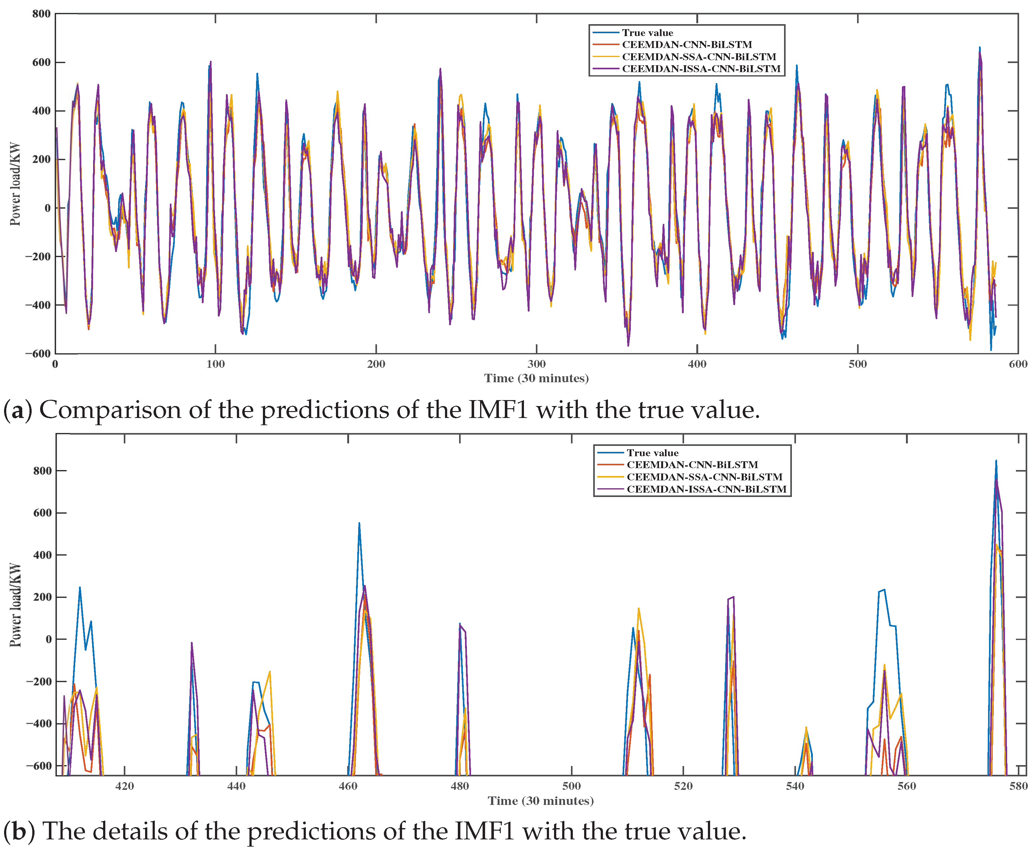
The reconstructed IMF1 and its prediction values obtained via CEEMDAN-CNN-BiLSTM, CEEMDAN-SSA-CNN-BiLSTM, and CEEMDAN-ISSA-CNN-BiLSTM are shown in Figure 10. From Figure 10, it can be seen that IMF1 shows strong volatility in time series analysis, and the traditional CNN-BiLSTM model is ineffective in predicting this data series. However, the prediction results are significantly improved after optimizing the model through the SSA and ISSA. From Figure 10b, it can be seen that ISSA optimization results can maintain high prediction accuracy in data peaks and valleys, better capture local features in power data, exhibit more stable performance, be less affected by volatility, and predict values closer to the actual results. It indicates that the adoption of the ISSA can not only effectively deal with the complex fluctuations in time series, but also enhance the robustness of the network and the prediction accuracy. In summary, the ISSA shows strong advantages in improving the performance of CNN-BiLSTM.

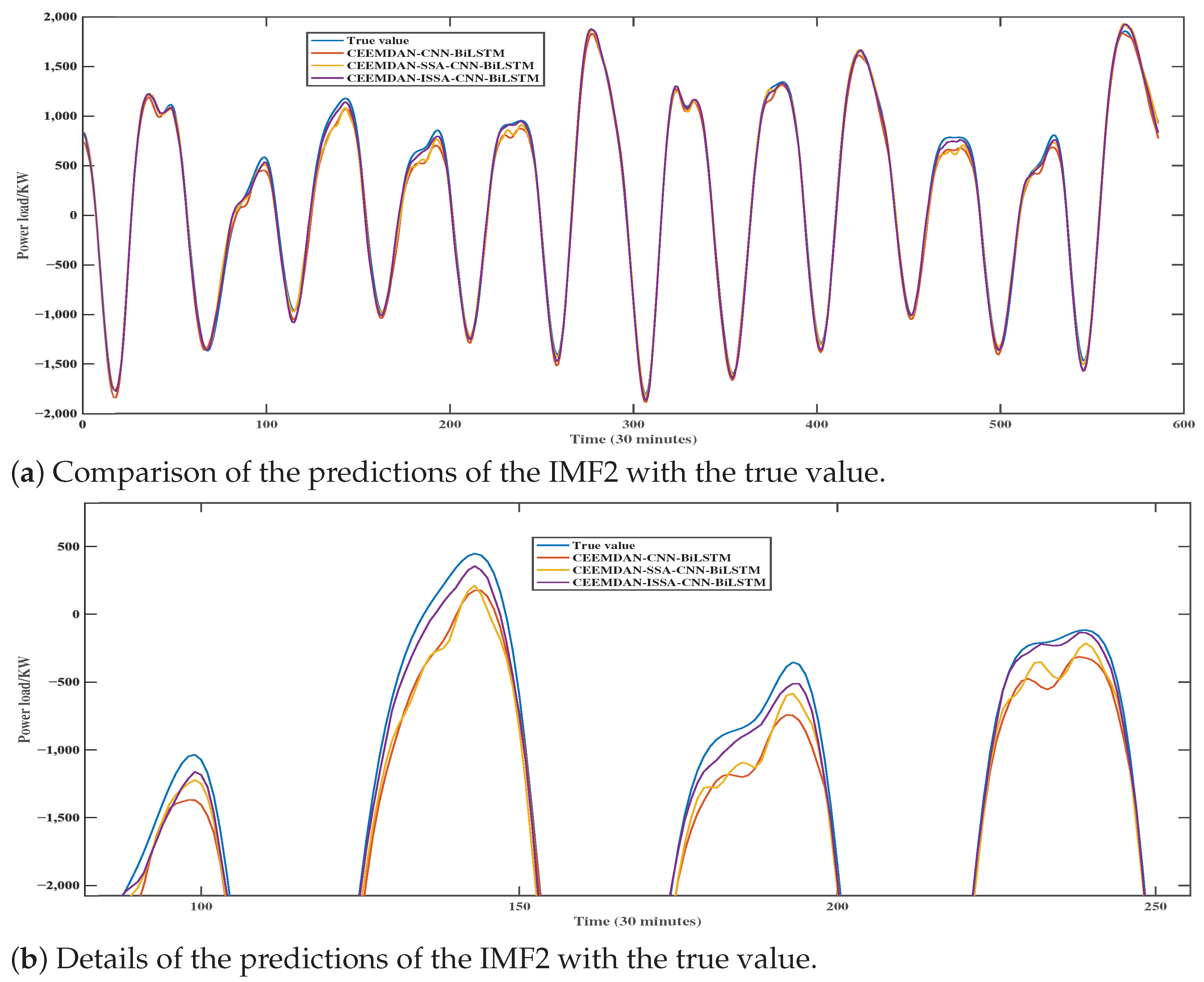
The reconstructed IMF2 and its prediction values obtained via CEEMDAN-CNN-BiLSTM, CEEMDAN-SSA-CNN-BiLSTM, and CEEMDAN-ISSA-CNN-BiLSTM are illustrated in Figure 11. From Figure 11, it can be seen that the IMF2 curve is smoother compared to IMF1, which implies that the IMF2 data are less volatile and relatively less difficult to predict. Observing the consistency between the predicted values and the true values of the models indicates that the three models can effectively capture the dynamic changes in time series. It can be seen from Figure 11b that, although the SSA and ISSA show some degree of improvement in prediction, the CNN-BiLSTM model optimized by the ISSA predicts results that are closer to the true values, with higher curve fitting and more extreme points similar to the true values. Overall, the ISSA-optimized method not only exhibits superior performance when dealing with complex and fluctuating IMF1 data, but also shows higher accuracy and reliability in the prediction of the relatively smooth IMF2.

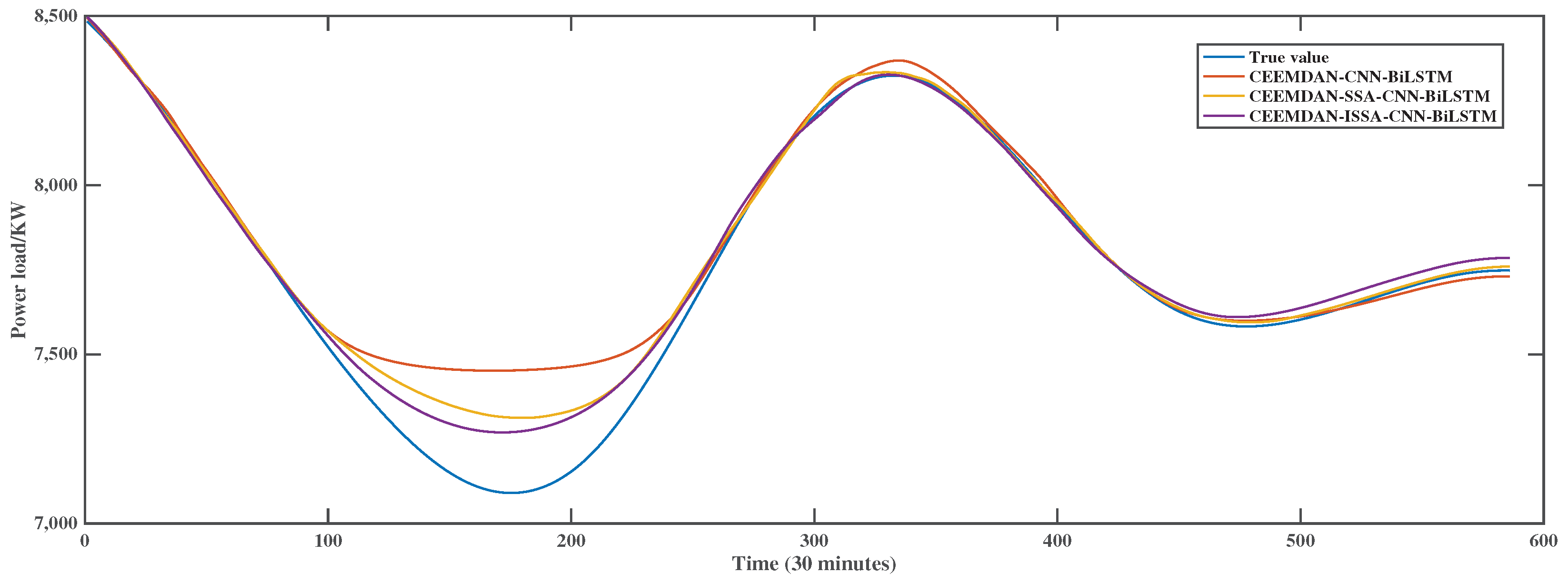
Figure 12 captures the reconstructed IMF3 and compares the prediction results of CEEMDAN-CNN-BiLSTM, CEEMDAN-SSA-CNN-BiLSTM, and CEEMDAN-ISSA-CNN-BiLSTM for this component. The IMF3 data are very smooth and less difficult to predict. Compared with CEEMDAN-CNN-BiLSTM and CEEMDAN-SSA-CNN-BiLSTM, the CEEMDAN-ISSA-CNN-BiLSTM model better grasps the laws of load changes, and the predicted curve is more in line with the actual load curve. The fitting effect near the extreme points of the sequence is better, the deviation and fluctuation are smaller, and the prediction ability is stronger.

3.4. Error Analysis

To verify the robustness and superiority of CEEMDAN-ISSA-CNN-BiLSTM, this section uses the final prediction results and compares the error metrics, the MAE, RMSE, and MAPE, to analyze the significant improvement of the proposed model compared to the alternative model.

Comparing the final prediction results of the three methods for original load data in Figure 13, we can see that each method performs well at both peak and off-peak hours, but each method performs slightly worse at peak levels compared to off-peak hours. The predictions of CEEMDAN-ISSA-CNN-BiLSTM are closest to the actual values at both peaks and troughs, CEEMDAN-SSA-CNN-BiLSTM is the second closest, and the unoptimized CEEMDAN-CNN-BiLSTM is furthest away from the actual values. Further validation of the need to optimize model parameters using the ISSA is required.

We conduct comprehensive comparisons between the proposed model and classical baseline models (LSTM, BiLSTM), as well as enhanced variants (CNN-LSTM, CNN-BiLSTM, EMD-CNN-BiLSTM, CEEMDAN-CNN-LSTM, CEEMDAN-CNN-BiLSTM). As shown in

Table 4. Results of evaluation indicators for nine forecasting models.

Method	MAE	RMSE	MAPE/%
LSTM	136.2837	172.9691	1.7710
BiLSTM	131.6981	166.7711	1.6982
CNN-LSTM	122.6703	163.6129	1.6022
CNN-BiLSTM	123.4603	165.9294	1.5567
EMD-CNN-BiLSTM	115.6594	145.3522	1.4440
CEEMDAN-CNN-LSTM	101.0761	131.7941	1.3079
CEEMDAN-CNN-BiLSTM	95.6848	127.2255	1.2567
CEEMDAN-SSA-CNN-BiLSTM	88.0911	115.1259	1.1441
CEEMDAN-ISSA-CNN-BiLSTM	76.3607	97.4285	0.9916

, the proposed model demonstrates significant reductions across three key performance metrics: root mean square error (RMSE), reflecting sensitivity to large prediction deviations, mean absolute error (MAE), measuring average absolute prediction errors, and mean absolute percentage error (MAPE), quantifying relative prediction accuracy. The proposed CEEMDAN-ISSA-CNN-BiLSTM model performs the best in all three indicators, with reductions of 44.0%, 43.7%, and 44.0% compared to the baseline LSTM model, respectively. Its advantages stem from the three-level collaborative mechanism.

(1) The CNN-BiLSTM architecture synergistically integrates parallel convolutional operations for spatial feature extraction and bidirectional LSTM layers for contextual temporal modeling, enabling the concurrent capture of spatiotemporal dynamics and bidirectional long-term dependencies in load sequences. Comparative evaluation against standalone LSTM architectures demonstrates a significant error reduction: a 9.4% lower MAE, a 4.1% reduced RMSE, and a 12.1% improvement in MAPE, attributable to enhanced multi-scale pattern recognition and adaptive temporal correlation modeling.

(2) The CEEMDAN technique effectively mitigates mode mixing phenomena in raw load signals while enhancing signal stationarity through adaptive noise injection. Comparative analysis reveals that the CEEMDAN-CNN-BiLSTM framework achieves significant error reduction across multiple metrics: Against the CNN-BiLSTM baseline, there is a 22.5% MAE, 23.3% RMSE, and 19.3% MAPE improvement. Versus the CNN-LSTM architecture, there is a 17.6% MAE, 19.4% RMSE, and 18.4% MAPE enhancement. And compared to EMD-CNN-BiLSTM, there is a 12.% MAE, 9.3% RMSE, and 9.4% MAPE improvement, showing superior performance. This performance superiority stems from the complete ensemble properties of CEEMDAN that eliminate residual noise contamination during decomposition coupled with CNN-BiLSTM’s dual capability in spatial feature extraction and bidirectional temporal modeling. The hybrid architecture demonstrates particular efficacy in resolving non-stationary load patterns through multi-scale signal decomposition and correlated component clustering.

(3) The ISSA framework enables adaptive hyperparameter optimization for CNN-BiLSTM architectures, effectively mitigating the subjective parameter configuration bias inherent in manual tuning processes. The comparative evaluation demonstrates that the CEEMDAN-ISSA-CNN-BiLSTM hybrid model achieves superior performance metrics: Against CEEMDAN-CNN-BiLSTM, it achieves a 20.2% MAE reduction, 23.4% RMSE improvement, and 21.1% MAPE enhancement. Versus CEEMDAN-SSA-CNN-BiLSTM, it achieves a 13.3% MAE, 15.4% RMSE, and 13.3% MAPE reduction. This optimization efficacy stems from the ISSA’s enhanced global search capabilities—integrating Lévy flight dynamics and golden sine position updating—which systematically explore high-dimensional hyperparameter spaces (learning rates, hidden units, kernel sizes) while avoiding local optima stagnation and reducing the manual intervention requirements.

In summary, the CEEMDAN-ISSA-CNN-BiLSTM prediction model proposed in this article has the most outstanding and stable predictive performance and can track the trend of historical load data well. In addition, the MAE evaluation value of the CEEMDAN-ISSA-CNN-BiLSTM model is the lowest, indicating that the average deviation between the predicted results of the proposed model and the true values is low, and the load prediction error at each moment is small, which helps the power grid dispatch department to allocate power generation resources more accurately. The minimum RMSE evaluation value indicates that the model has less extreme prediction bias, more stable prediction results, and can reduce the power grid frequency fluctuations or insufficient reserve capacity caused by extreme errors. The minimum MAPE evaluation value indicates that the model has relatively low relative errors at different load levels and can perform more robustly in both high-load and low-load forecasting scenarios. However, the model may have limitations in extreme events such as sudden power outages, mainly due to limitations in training data coverage, computational latency, and the lack of explicit modeling of multi-energy interaction mechanisms. In the future, its engineering applicability can be further improved through adversarial sample generation, lightweight end-to-end architecture design, and multimodal data fusion strategies.

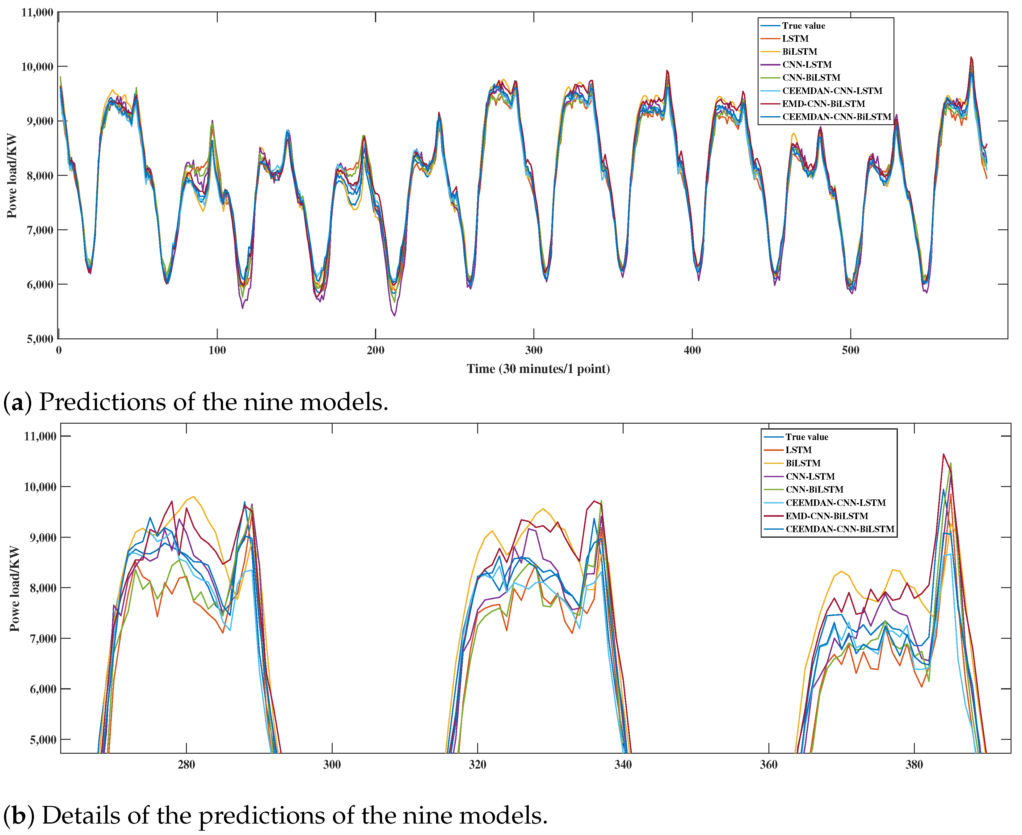
As shown in Figure 14, the performance of each model in the test set prediction is good; the prediction curves are closely connected with the real curves most of the time, which shows the strong ability of the models to grasp and pump the main trends and cyclic variations of the data, and distinctly demonstrates their respective characteristics and advantages. Among them, CEEMDAN-ISSA-CNN-LSTM has the highest consistency between predictions and actual observations, and the prediction error is smaller than that of the other eight compared models, which is consistent with the results shown in Table 4.

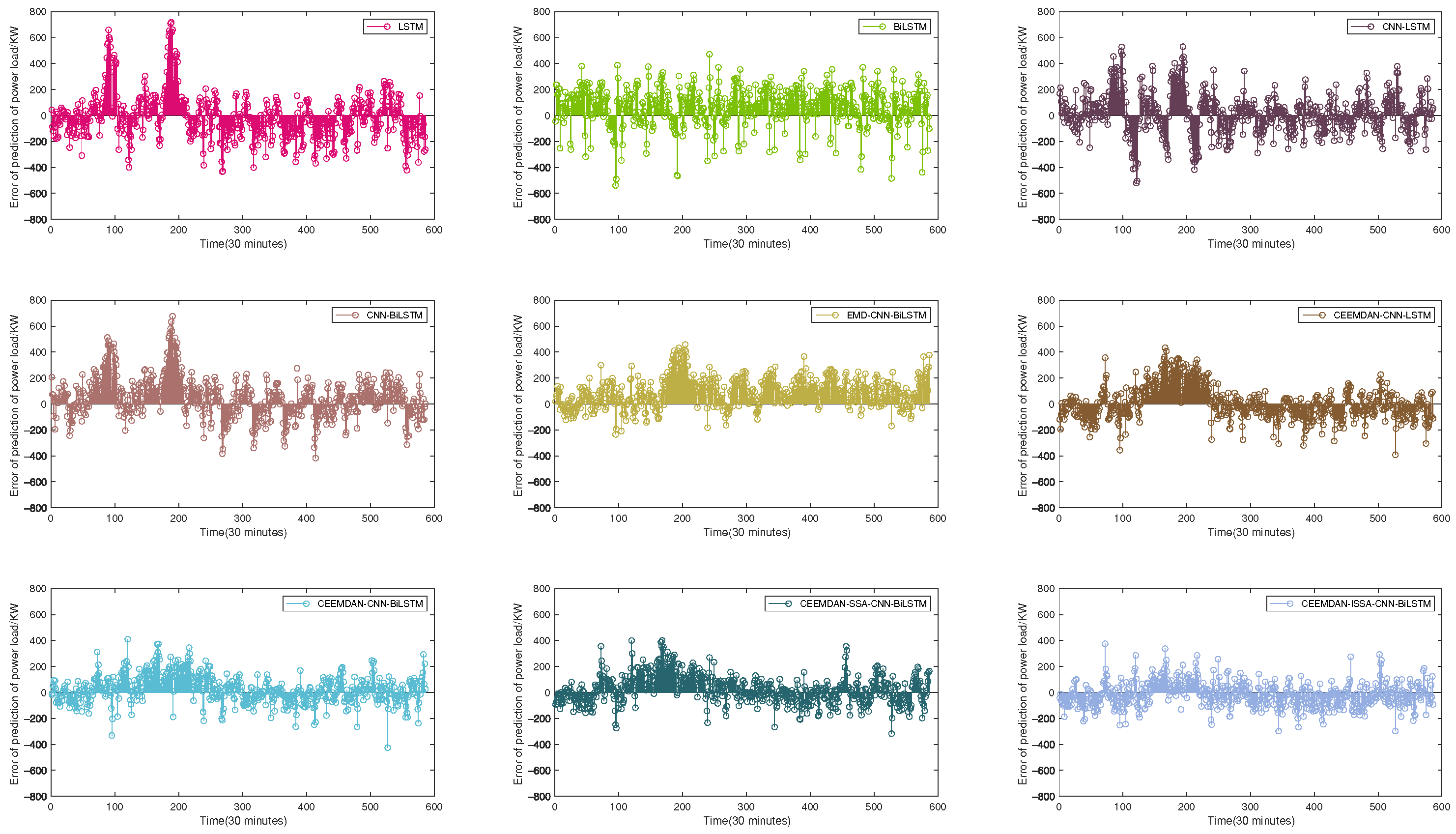
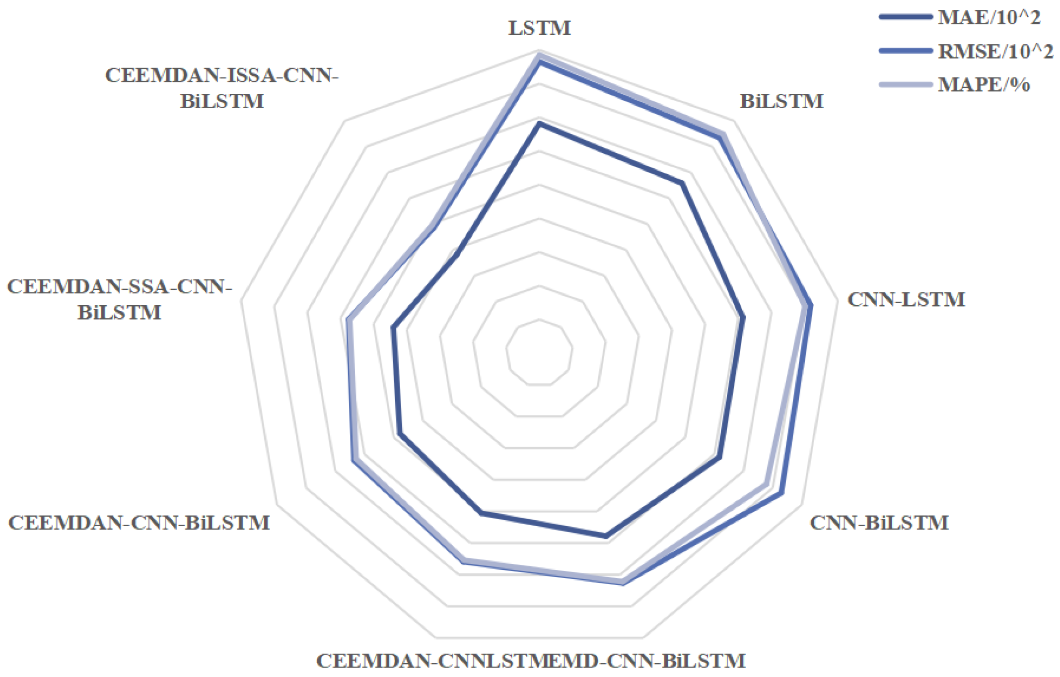
To more intuitively compare the prediction errors of the models, residual distribution graphs illustrating model accuracy variations are shown in Figure 15, and a radar chart of the performance criteria is shown in Figure 16. Figure 15 reveals distinct patterns: Each model occurs predominantly during off-peak hours, where load fluctuations are minimal. The models occasionally overfit to minor noise in low-demand periods, leading to conservative over-predictions. Underestimation is observed during abrupt load spikes in peak hours. Rapid demand surges caused by factors like sudden weather changes or commercial activity are not fully captured, resulting in a lagged response. As shown in Figure 10, Figure 11, Figure 12 and Figure 13, mid-frequency IMFs exhibit smaller residuals due to their smoother trends, while high-frequency IMFs contribute to larger errors during volatile periods. In addition, we find that LSTM, CNN-BiLSTM, CNN-BiLSTM, EMD-CNN-BiLSTM, CEEEMDAN-CNN-BiLSTM, and CEEEMDAN-SSA-CNN-BiLSTM all have locally large residuals with positive signs from the 100th to the 200th time point in the testing data, but CEEEMDAN-SSA-CNN-BiLSTM performs robustly with the uniform and small residual terms. Overall, CEEEMDAN-SSA-CNN-BiLSTM maintains a relatively small jitter of the residuals of prediction, performing better than the other eight methods. As shown in Figure 16, the CEEMDAN-SSA-CNN-BiLSTM performs well in all three key evaluation indexes, and the specific data values are all the smallest, which indicates that the model has a significant advantage in data processing, feature extraction, and prediction, and the prediction accuracy is better than that of the other eight comparison models.

To enhance peak-hour accuracy, we may take the following measures:

• Dynamic Hyperparameter Tuning: Integration of real-time optimization where the ISSA adjusts model parameters hourly based on incoming data streams.
• Exogenous Variable Integration: Incorporation of weather forecasts, holiday calendars, and economic indicators to contextualize abrupt load changes.
• Hybrid Attention Mechanisms: Use of temporal attention layers in BiLSTM to prioritize recent peak-hour trends during decoding.

4. Discussion

Deploying deep learning models such as CEEMDAN-ISSA-CNN-BiLSTM in large-scale power grids faces multiple challenges. Firstly, the scalability issue of dynamic system models is particularly prominent, as their computational burden mainly stems from solving the parameters in large-scale networks, and existing research lacks practical case studies to verify their scalability [85]. For example, power system simulation (such as chip-level power network analysis) typically involves a network of millions of nodes, requiring efficient algorithms to reduce memory and computation time. In addition, the model needs to balance complexity and practicality. The choice of modeling methods such as linear/nonlinear, static/dynamic, and deterministic/probabilistic methods directly affects the computational resource requirements and result accuracy. It is recommended to alleviate scalability bottlenecks through model reduction (such as equivalent network representation) or distributed computing frameworks (such as cloud platform collaborative simulation).

Complex models such as CEEMDAN-ISSA-CNN-BiLSTM may face latency issues in real-time applications. Although existing power system simulation tools, such as production cost models, can support short-term operational planning, further optimization of algorithm efficiency is needed to meet real-time operational requirements. Possible optimization directions include hardware acceleration, utilizing GPU/TPU parallel computing to accelerate deep learning inference, and hybrid modeling, combining optimization methods with machine learning to embed lightweight models at critical stages. In addition, the asynchronous processing of real-time data streams and the edge computing architecture could reduce the burden of centralized computing.

CEEMDAN-ISSA-CNN-BiLSTM may outperform single deep learning models (such as LSTM) in predicting high-volatility power load sources through a cascaded structure of decomposition optimization time series modeling. Although the computational cost of this model is higher than that of the single-network models, its advantages in multi-time scale feature extraction and nonlinear relationship modeling may be competitive in high-precision demand scenarios. Future research will continue to explore how to apply the CEEMDAN-ISSA-CNN-BiLSTM model to real-time prediction systems to achieve dynamic scheduling and optimized operation of power systems. This includes developing efficient algorithms and data processing techniques to ensure that the model can quickly respond and adapt to changes in real-time environments and combining multiple sources of data such as meteorological data and socio-economic data to improve the comprehensiveness of predictions. By collecting and processing these data in real time, the model can better adapt to environmental changes and improve the real-time reliability of predictions.

CEEMDAN-ISSA-CNN-BiLSTM has shown potential in power system prediction and optimization, but its large-scale deployment relies on algorithm efficiency improvement, hardware resource adaptation, and interdisciplinary collaborative innovation. In the future, we need to focus on breaking through the bottleneck of real-time performance and promote the implementation of technology through hybrid modeling.

5. Conclusions

This study proposes a CEEMDAN-ISSA-CNN-BiLSTM model for STLF. The model addresses three critical challenges: the non-stationary of load data, inefficient hyperparameter tuning, and limited feature extraction. Its “decomposition–optimization–prediction” framework systematically resolves these issues. Firstly, the CEEMDAN method and sample entropy method, respectively, decompose and reconstruct the load data into IMFs representing different frequency components to enhance signal-to-noise ratios (SNR). This step reduces data complexity and improves model interpretability. We improve the SSA to optimize CNN-BiLSTM hyperparameters. The traditional SSA often traps models in local optima, causing prediction bias of CNN-BiLSTM. Our ISSA introduces three strategies:

• Good point set initialization, which ensures balanced population distribution.
• The golden sine strategy, which updates discoverer positions for faster convergence.
• Lévy flight, which enhances global search during population movement.

These upgrades reduce computational costs and improve optimization accuracy for selecting the hyperparameters in CNN-BiLSTM. Tests show that the ISSA lowers the MAPE by 10% compared to the SSA, combing with CNN-BiLSTM for STLF, where both the algorithms improve at least 10% of the MAPE compared to the hybrid models without an intelligent optimization algorithm. The CNN-BiLSTM hybrid model captures both local patterns and long-term dependencies in load sequences. By combining the local feature extraction of a CNN with the bidirectional temporal modeling of BiLSTM, the model achieves superior performance, with MAE, RMSE, and MAPE values of 76.36, 97.43, and 0.99%, respectively. These results outperform eight benchmark models. This framework systematically enhances prediction accuracy by addressing multi-scale periodic patterns and nonlinear disturbances in load data.

The proposed model holds substantial promise for real-world energy management. Accurate STLF enables utilities to optimize generation scheduling, reduce operational risks, and enhance demand-side response, particularly in dynamic environments with renewable energy integration. Lower forecasting errors (e.g., 0.99% MAPE) minimize over- or under-generation costs and improve fuel procurement planning. This is critical for grids integrating renewable energy. While the computational complexity of the model poses challenges for real-time deployment, strategies like GPU acceleration or edge computing (as discussed) could facilitate adoption in large-scale smart grids.

In future research, we will extend the model to multi-horizon predictions to support broader grid planning. For external factors, we may incorporate weather, holidays, and socio-economic data to improve robustness against exogenous variables. In addition, we will explore lightweight architectures (e.g., knowledge distillation) or adaptive CEEMDAN variants to reduce training time without sacrificing accuracy and validate the model in real-time systems with streaming data and hardware acceleration (e.g., TPUs) to address latency challenges. By addressing these directions, future work could further bridge the gap between theoretical innovation and practical implementation in smart grid analytics.

References

1. Luo, J.; Hong, T.; Gao, Z.; Fang, S.C. A robust support vector regression model for electric load forecasting. Int. J. Forecast. 2023, 39, 1005–1020. [Google Scholar] [CrossRef]
2. Tsalikidis, N.; Mystakidis, A.; Tjortjis, C.; Koukaras, P.; Ioannidis, D. Energy load forecasting: One-step ahead hybrid model utilizing ensembling. Computing 2024, 106, 241–273. [Google Scholar] [CrossRef]
3. Kantardzic, M.; Gavranovic, H.; Gavranovic, N.; Dzafic, I.; Hu, H. Improved short term energy load forecasting using Web-based social networks. Soc. Netw. 2015, 4, 119–131. [Google Scholar] [CrossRef]
4. Almeshaiei, E.; Soltan, H. A methodology for electric power load forecasting. Alex. Eng. J. 2011, 50, 137–144. [Google Scholar] [CrossRef]
5. Ryu, S.; Noh, J.; Kim, H. Deep neural network based demand side short term load forecasting. Energies 2016, 10, 3. [Google Scholar] [CrossRef]
6. Zhang, L.; Jie, J.; Mingche, L. Adaptive parallel decision deep neural network for high-speed equalization. Opt. Express 2023, 31, 22001–22011. [Google Scholar] [CrossRef]
7. Hu, H.; Xia, X.; Luo, Y.; Zhang, C.; Nazir, M.S.; Peng, T. Development and application of an evolutionary deep learning framework of LSTM based on improved grasshopper optimization algorithm for short-term load forecasting. J. Build. Eng. 2022, 57, 104975. [Google Scholar] [CrossRef]
8. Song, K.B.; Baek, Y.S.; Hong, D.H.; Jang, G. Short-term load forecasting for the holidays using fuzzy linear regression method. IEEE Trans. Power Syst. 2005, 20, 96–101. [Google Scholar] [CrossRef]
9. Pappas, S.S.; Ekonomou, L.; Karamousantas, D.C.; Chatzarakis, G.; Katsikas, S.; Liatsis, P. Electricity demand loads modeling using AutoRegressive Moving Average (ARMA) models. Energy 2008, 33, 1353–1360. [Google Scholar] [CrossRef]
10. Mi, J.; Fan, L.; Duan, X.; Qiu, Y. Short-term power load forecasting method based on improved exponential smoothing grey model. Math. Probl. Eng. 2018, 2018, 3894723. [Google Scholar] [CrossRef]
11. Hippert, H.S.; Pedreira, C.E.; Souza, R.C. Neural networks for short-term load forecasting: A review and evaluation. IEEE Trans. Power Syst. 2001, 16, 44–55. [Google Scholar] [CrossRef]
12. Song, J.; Wang, J.; Lu, H. A novel combined model based on advanced optimization algorithm for short-term wind speed forecasting. Appl. Energy 2018, 215, 643–658. [Google Scholar] [CrossRef]
13. Zhao, H.X.; Magoulès, F. A review on the prediction of building energy consumption. Renew. Sustain. Energy Rev. 2012, 16, 3586–3592. [Google Scholar] [CrossRef]
14. Ruxue, L.; Shumin, L.; Miaona, Y.; Jican, L. Load forecasting based on weighted grey relational degree and improved ABC-SVM. J. Electr. Eng. Technol. 2021, 16, 2191–2200. [Google Scholar] [CrossRef]
15. Chen, Y.; Xu, P.; Chu, Y.; Li, W.; Wu, Y.; Ni, L.; Bao, Y.; Wang, K. Short-term electrical load forecasting using the Support Vector Regression (SVR) model to calculate the demand response baseline for office buildings. Appl. Energy 2017, 195, 659–670. [Google Scholar] [CrossRef]
16. Tay, F.E.; Cao, L. Application of support vector machines in financial time series forecasting. Omega 2001, 29, 309–317. [Google Scholar] [CrossRef]
17. Zhang, G.; Hu, M.Y. Neural network forecasting of the British pound/US dollar exchange rate. Omega 1998, 26, 495–506. [Google Scholar] [CrossRef]
18. Chiang, W.C.; Urban, T.L.; Baldridge, G.W. A neural network approach to mutual fund net asset value forecasting. Omega 1996, 24, 205–215. [Google Scholar] [CrossRef]
19. Ojha, V.K.; Abraham, A.; Snášel, V. Metaheuristic design of feedforward neural networks: A review of two decades of research. Eng. Appl. Artif. Intell. 2017, 60, 97–116. [Google Scholar] [CrossRef]
20. Velasco, L.C.P.; Arnejo, K.A.S.; Macarat, J.S.S.; Tinam-isan, M.A.C. Hour-ahead electric load forecasting using artificial neural networks. In Proceedings of the Sixth International Congress on Information and Communication Technology: ICICT 2021, London, UK, 25–26 February 2021; Springer: Berlin/Heidelberg, Germany, 2022; Volume 3, pp. 843–855. [Google Scholar]
21. Chitalia, G.; Pipattanasomporn, M.; Garg, V.; Rahman, S. Robust short-term electrical load forecasting framework for commercial buildings using deep recurrent neural networks. Appl. Energy 2020, 278, 115410. [Google Scholar] [CrossRef]
22. Yazici, I.; Beyca, O.F.; Delen, D. Deep-learning-based short-term electricity load forecasting: A real case application. Eng. Appl. Artif. Intell. 2022, 109, 104645. [Google Scholar] [CrossRef]
23. Almalaq, A.; Edwards, G. A review of deep learning methods applied on load forecasting. In Proceedings of the 2017 16th IEEE international conference on machine learning and applications (ICMLA), Cancun, Mexico, 18–21 December 2017; pp. 511–516. [Google Scholar]
24. Bouktif, S.; Fiaz, A.; Ouni, A.; Serhani, M.A. Optimal deep learning lstm model for electric load forecasting using feature selection and genetic algorithm: Comparison with machine learning approaches. Energies 2018, 11, 1636. [Google Scholar] [CrossRef]
25. Mocanu, E.; Nguyen, P.H.; Gibescu, M.; Kling, W.L. Deep learning for estimating building energy consumption. Sustain. Energy Grids Netw. 2016, 6, 91–99. [Google Scholar] [CrossRef]
26. Rahman, A.; Srikumar, V.; Smith, A.D. Predicting electricity consumption for commercial and residential buildings using deep recurrent neural networks. Appl. Energy 2018, 212, 372–385. [Google Scholar] [CrossRef]
27. Hochreiter, S.; Schmidhuber, J. Long short-term memory. Neural Comput. 1997, 9, 1735–1780. [Google Scholar] [CrossRef]
28. Liu, S.; Kong, Z.; Huang, T.; Du, Y.; Xiang, W. An ADMM-LSTM framework for short-term load forecasting. Neural Netw. 2024, 173, 106150. [Google Scholar] [CrossRef]
29. Wang, J.; Jiang, L.; Wang, L. Prediction of China’s Polysilicon Prices: A Combination Model Based on Variational Mode Decomposition, Sparrow Search Algorithm and Long Short-Term Memory. Mathematics 2024, 12, 3690. [Google Scholar] [CrossRef]
30. Wang, M.; Wang, Z.; Lu, J.; Lin, J.; Wang, Z. E-LSTM: An efficient hardware architecture for long short-term memory. IEEE J. Emerg. Sel. Top. Circuits Syst. 2019, 9, 280–291. [Google Scholar] [CrossRef]
31. Fürst, K.; Chen, P.; Gu, I.Y.H. Hierarchical LSTM-Based Classification of Household Heating Types Using Measurement Data. IEEE Trans. Smart Grid 2023, 15, 2261–2270. [Google Scholar] [CrossRef]
32. Zeng, B.; Qiu, Y.; Yang, X.; Chen, W.; Xie, Y.; Wang, Y.; Jiang, P. Research on short-term power load forecasting method based on multi-factor feature analysis and LSTM. J. Phys. Conf. Ser. 2023, 2425, 012068. [Google Scholar] [CrossRef]
33. Marino, D.L.; Amarasinghe, K.; Manic, M. Building energy load forecasting using deep neural networks. In Proceedings of the IECON 2016—42nd Annual Conference of the IEEE Industrial Electronics Society, Florence, Italy, 24–27 October 2016; pp. 7046–7051. [Google Scholar]
34. Yan, Q.; Lu, Z.; Liu, H.; He, X.; Zhang, X.; Guo, J. An improved feature-time Transformer encoder-Bi-LSTM for short-term forecasting of user-level integrated energy loads. Energy Build. 2023, 297, 113396. [Google Scholar] [CrossRef]
35. Chen, S.; Chen, B.; Shu, P.; Wang, Z.; Chen, C. Real-time unmanned aerial vehicle flight path prediction using a bi-directional long short-term memory network with error compensation. J. Comput. Des. Eng. 2023, 10, 16–35. [Google Scholar] [CrossRef]
36. Ahmad, A.S.; Hassan, M.Y.; Abdullah, M.P.; Rahman, H.A.; Hussin, F.; Abdullah, H.; Saidur, R. A review on applications of ANN and SVM for building electrical energy consumption forecasting. Renew. Sustain. Energy Rev. 2014, 33, 102–109. [Google Scholar] [CrossRef]
37. Li, T.; Hua, M.; Wu, X. A hybrid CNN-LSTM model for forecasting particulate matter (PM 2.5). IEEE Access 2020, 8, 26933–26940. [Google Scholar] [CrossRef]
38. Guo, X.; Zhao, Q.; Zheng, D.; Ning, Y.; Gao, Y. A short-term load forecasting model of multi-scale CNN-LSTM hybrid neural network considering the real-time electricity price. Energy Rep. 2020, 6, 1046–1053. [Google Scholar] [CrossRef]
39. Javed, U.; Ijaz, K.; Jawad, M.; Khosa, I.; Ansari, E.A.; Zaidi, K.S.; Rafiq, M.N.; Shabbir, N. A novel short receptive field based dilated causal convolutional network integrated with Bidirectional LSTM for short-term load forecasting. Expert Syst. Appl. 2022, 205, 117689. [Google Scholar] [CrossRef]
40. Thakre, P.; Khedkar, M.; Vardhan, B.S. A Comparative Analysis of Short Term Load Forecasting Using LSTM, CNN, and Hybrid CNN-LSTM. In Proceedings of the International Symposium on Sustainable Energy and Technological Advancements, Shillong, India, 24–25 February 2023; pp. 171–181. [Google Scholar]
41. Liao, R.; Ren, J.; Ji, C. Research on Short Term Power Load Forecasting Based on Wavelet and BiLSTM. In Proceedings of the International Conference on 6GN for Future Wireless Networks, Harbin, China, 17–18 December 2023; pp. 53–65. [Google Scholar]
42. Xiaoyan, H.; Bingjie, L.; Jing, S.; Hua, L.; Guojing, L. A novel forecasting method for short-term load based on TCN-GRU model. In Proceedings of the 2021 IEEE International Conference on Energy Internet (ICEI), Southampton, UK, 27–29 September 2021; pp. 79–83. [Google Scholar]
43. Li, T.; Zhang, X.; Zhao, H.; Xu, J.; Chang, Y.; Yang, S. A dual-head output network attack detection and classification approach for multi-energy systems. Front. Energy Res. 2024, 12, 1367199. [Google Scholar] [CrossRef]
44. Zenkner, G.; Navarro-Martinez, S. A flexible and lightweight deep learning weather forecasting model. Appl. Intell. 2023, 53, 24991–25002. [Google Scholar] [CrossRef]
45. Li, Y. Research on Load Forecasting of Power System Based on Deep Learning. Int. J. Comput. Sci. Inf. Technol. 2024, 3, 336–347. [Google Scholar] [CrossRef]
46. Zhang, C.; Zhou, J.; Li, C.; Fu, W.; Peng, T. A compound structure of ELM based on feature selection and parameter optimization using hybrid backtracking search algorithm for wind speed forecasting. Energy Convers. Manag. 2017, 143, 360–376. [Google Scholar] [CrossRef]
47. Meng, Z.; Xie, Y.; Sun, J. Short-term load forecasting using neural attention model based on EMD. Electr. Eng. 2022, 104, 1857–1866. [Google Scholar] [CrossRef]
48. Azam, M.F.; Younis, M.S. Multi-horizon electricity load and price forecasting using an interpretable multi-head self-attention and EEMD-based framework. IEEE Access 2021, 9, 85918–85932. [Google Scholar] [CrossRef]
49. Wang, Y.; Zhao, K.; Hao, Y.; Yao, Y. Short-term wind power prediction using a novel model based on butterfly optimization algorithm-variational mode decomposition-long short-term memory. Appl. Energy 2024, 366, 123313. [Google Scholar] [CrossRef]
50. Kaur, S.; Bala, A.; Parashar, A. A multi-step electricity prediction model for residential buildings based on ensemble Empirical Mode Decomposition technique. Sci. Technol. Energy Transit. 2024, 79, 7. [Google Scholar] [CrossRef]
51. Ran, P.; Dong, K.; Liu, X.; Wang, J. Short-term load forecasting based on CEEMDAN and Transformer. Electr. Power Syst. Res. 2023, 214, 108885. [Google Scholar] [CrossRef]
52. Huang, J.; Li, C.; Huang, Z.; Liu, P.X. A decomposition-based approximate entropy cooperation long short-term memory ensemble model for short-term load forecasting. Electr. Eng. 2022, 104, 1515–1525. [Google Scholar] [CrossRef]
53. Han, J.; Zeng, P. Residual BiLSTM based hybrid model for short-term load forecasting in buildings. J. Build. Eng. 2025, 99, 111593. [Google Scholar] [CrossRef]
54. Liu, K.; Ruan, J.; Zhao, X.; Liu, G. Short-term Load Forecasting Method Based on Sparrow Search Optimized Attention-GRU. Proc. CSU-EPSA 2022, 34, 99–106. [Google Scholar]
55. Nwankpa, C.E. Advances in optimisation algorithms and techniques for deep learning. Adv. Sci. Technol. Eng. Syst. J. 2020, 5, 563–577. [Google Scholar] [CrossRef]
56. Wang, D.; Tan, D.; Liu, L. Particle swarm optimization algorithm: An overview. Soft Comput. 2018, 22, 387–408. [Google Scholar] [CrossRef]
57. Zhou, M.; Yu, J.; Wang, M.; Quan, W.; Bian, C. Research on the combined forecasting model of cooling load based on IVMD-WOA-LSSVM. Energy Build. 2024, 317, 114339. [Google Scholar] [CrossRef]
58. Mirjalili, S.; Mirjalili, S.M.; Lewis, A. Grey wolf optimizer. Adv. Eng. Softw. 2014, 69, 46–61. [Google Scholar] [CrossRef]
59. Xue, J.; Shen, B. A novel swarm intelligence optimization approach: Sparrow search algorithm. Syst. Sci. Control Eng. 2020, 8, 22–34. [Google Scholar] [CrossRef]
60. Wen, J.; Wang, Z. Short-Term Power Load Forecasting with Hybrid TPA-BiLSTM Prediction Model Based on CSSA. CMES-Comput. Model. Eng. Sci. 2023, 136. [Google Scholar] [CrossRef]
61. Tang, M.; Wang, C.; Qiu, J.; Li, H.; Guo, X.; Sheng, W. Short-term load forecasting of electric vehicle charging stations accounting for multifactor IDBO hybrid models. Energies 2024, 17, 2831. [Google Scholar] [CrossRef]
62. Xie, X.; Huang, Y. Displacement Prediction Method for Bank Landslide Based on SSA-VMD and LSTM Model. Mathematics 2024, 12, 1001. [Google Scholar] [CrossRef]
63. Gharehchopogh, F.S.; Namazi, M.; Ebrahimi, L.; Abdollahzadeh, B. Advances in sparrow search algorithm: A comprehensive survey. Arch. Comput. Methods Eng. 2023, 30, 427–455. [Google Scholar] [CrossRef]
64. Chen, Y.; Li, J.; Zhang, L. Learning sparrow algorithm with non-uniform search for global optimization. Int. J. Swarm Intell. Res. (IJSIR) 2023, 14, 1–31. [Google Scholar] [CrossRef]
65. Abdulsaed, E.H.; Alabbas, M.; Khudeyer, R.S. Optimizing the Architecture of Convolutional Neural Networks Using Modified Salp Swarm Algorithm. J. Al-Qadisiyah Comput. Sci. Math. 2024, 16, 124–136. [Google Scholar] [CrossRef]
66. Qinghua, M.; Qiang, Z. Improved sparrow algorithm combining Cauchy mutation and opposition-based learning. J. Front. Comput. Sci. Technol. 2021, 15, 1155. [Google Scholar]
67. Kundu, T.; Deepmala; Jain, P.K. A hybrid salp swarm algorithm based on TLBO for reliability redundancy allocation problems. Appl. Intell. 2022, 52, 12630–12667. [Google Scholar] [CrossRef] [PubMed]
68. Liu, J.; He, Q.; Yue, Z.; Pei, Y. A Hybrid Strategy-Improved SSA-CNN-LSTM Model for Metro Passenger Flow Forecasting. Mathematics 2024, 12, 3929. [Google Scholar] [CrossRef]
69. Sun, S.; Yu, P.; Xing, J.; Cheng, Y.; Yang, S.; Ai, Q. Short-Term Wind Power Prediction Based on ICEEMDAN-SE-LSTM Neural Network Model with Classifying Seasonal. Energy Eng. 2023, 120, 2761. [Google Scholar] [CrossRef]
70. Torres, M.E.; Colominas, M.A.; Schlotthauer, G.; Flandrin, P. A complete ensemble empirical mode decomposition with adaptive noise. In Proceedings of the 2011 IEEE International Conference on Acoustics, Speech and Signal Processing (ICASSP), Seoul, Republic of Korea, 14–19 April 2011; pp. 4144–4147. [Google Scholar]
71. Wang, Y.; Xu, C.; Wang, Y.; Cheng, X. A comprehensive diagnosis method of rolling bearing fault based on CEEMDAN-DFA-improved wavelet threshold function and QPSO-MPE-SVM. Entropy 2021, 23, 1142. [Google Scholar] [CrossRef] [PubMed]
72. Owusu Junior, P.; Frimpong, S.; Adam, A.M.; Agyei, S.K.; Gyamfi, E.N.; Agyapong, D.; Tweneboah, G. COVID-19 as Information Transmitter to Global Equity Markets: Evidence from CEEMDAN-Based Transfer Entropy Approach. Math. Probl. Eng. 2021, 2021, 8258778. [Google Scholar] [CrossRef]
73. Richman, J.S.; Moorman, J.R. Physiological time-series analysis using approximate entropy and sample entropy. Am. J. Physiol.-Heart Circ. Physiol. 2000, 278, H2039–H2049. [Google Scholar] [CrossRef]
74. Tian, Z.; Chen, H. A novel decomposition-ensemble prediction model for ultra-short-term wind speed. Energy Convers. Manag. 2021, 248, 114775. [Google Scholar] [CrossRef]
75. Zhang, J.; Gao, Z.; Li, Y.; Jiang, Y. A deep learning method for convective weather forecasting: CNN-BiLSTM-AM (version 1.0). Geosci. Model Dev. Discuss. 2023, 2023, 1–32. [Google Scholar]
76. Imani, M. Electrical load-temperature CNN for residential load forecasting. Energy 2021, 227, 120480. [Google Scholar] [CrossRef]
77. Liu, H.; Li, Z.; Li, C.; Shao, L.; Li, J. Research and application of short-term load forecasting based on CEEMDAN-LSTM modeling. Energy Rep. 2024, 12, 2144–2155. [Google Scholar] [CrossRef]
78. Huang, J.; Zhang, X.; Jiang, X. Short-term power load forecasting based on the CEEMDAN-TCN-ESN model. PLoS ONE 2023, 18, e0284604. [Google Scholar] [CrossRef] [PubMed]
79. Zheng, G.Q.; Kong, L.R.; Su, Z.E.; Hu, M.S.; Wang, G.D. Approach for short-term power load prediction utilizing the ICEEMDAN–LSTM–TCN–bagging model. J. Electr. Eng. Technol. 2025, 20, 231–243. [Google Scholar] [CrossRef]
80. Quansah, P.K.; Tenkorang, E.K.A. Short-term load forecasting using A particle-swarm optimized multi-head attention-augmented CNN-LSTM network. arXiv 2023, arXiv:2309.03694. [Google Scholar]
81. Kontogiannis, D.I. Design Strategies Towards the Enhancement of Short-Term Forecasting in the Energy Sector. Ph.D. Thesis, University of Thessaly (UTH), Volos, Greace, 2023. [Google Scholar]
82. Cerqueira, V.; Torgo, L.; Mozetič, I. Evaluating time series forecasting models: An empirical study on performance estimation methods. Mach. Learn. 2020, 109, 1997–2028. [Google Scholar] [CrossRef]
83. Liu, M.; Li, Y.; Hu, J.; Wu, X.; Deng, S.; Li, H. A New Hybrid Model Based on SCINet and LSTM for Short-Term Power Load Forecasting. Energies 2023, 17, 95. [Google Scholar] [CrossRef]
84. Olawuyi, A.; Ajewole, T.; Lawal, M.; Awofolaju, T. Enhancing Load Prediction Accuracy using Optimized Support Vector Regression Models. J. Digit. Food Energy Water Syst. 2023, 4, 2847. [Google Scholar] [CrossRef]
85. Abdelmalak, M.; Venkataramanan, V.; Macwan, R. A survey of cyber-physical power system modeling methods for future energy systems. IEEE Access 2022, 10, 99875–99896. [Google Scholar] [CrossRef]
Figure 3. CNN framework chart.
Mathematics 13 00813 g003
Figure 4. LSTM framework chart.
Mathematics 13 00813 g004
Figure 7. Original power load sequences.
Mathematics 13 00813 g007
Figure 8. Composition by CEEMDAN.
Mathematics 13 00813 g008
Figure 9. Reconstruction by sample entropy.
Mathematics 13 00813 g009
Figure 10. Predictions of IMF1 components by different models (a) and detailed view (b).
Mathematics 13 00813 g010
Figure 11. Predictions of Co-IMF2 components by different models (a) and detailed view (b).
Mathematics 13 00813 g011
Figure 12. Comparison of the predictions of the IMF3 with the true value.
Mathematics 13 00813 g012
Figure 13. Predictions and details of the proposed model and two comparative models.
Mathematics 13 00813 g013
Figure 14. Predictions and details of the nine models.
Mathematics 13 00813 g014
Figure 15. Residual distributions of each model.
Mathematics 13 00813 g015
Figure 16. MAE, RMSE, and MAPE of nine models.
Mathematics 13 00813 g016