An Improvement of the Alternating Direction Method of Multipliers to Solve the Convex Optimization Problem

Abstract

The alternating direction method is one of the attractive approaches for solving convex optimization problems with linear constraints and separable objective functions. Experience with applications has shown that the number of iterations depends significantly on the penalty parameter for the linear constraint. The penalty parameters in the classical alternating direction method are a constant. In this paper, an improved alternating direction method is proposed, which not only adaptively adjusts the penalty parameters per iteration based on the iteration message but also adds relaxation factors to the Lagrange multiplier update steps. Preliminary numerical experiments show that the technique of adaptive adjusting of the penalty parameters per iteration and attaching relaxation factors in the Lagrange multiplier updating steps are effective in practical applications.

1. Introduction

Many problems in the fields of signal and image processing, machine learning, medical image reconstruction, computer vision, and network communications [1,2,3,4,5,6,7,8] can be reduced to solving the following convex optimization problem with linear constraints:

$$\min \left\{f(x)+g(y)|Ax+By=b,x\in \mathcal{X},y\in \mathcal{Y}\right\}$$

(1)

where $A\in {ℝ}^{m\times m_1}$ and $B\in {ℝ}^{m\times m_2}$ are the given matrices; $b\in {ℝ}^m$ is the given vector; $f:{ℝ}^{m_1}\to ℝ$ and $g:{ℝ}^{m_2}\to ℝ$ are continuous closed convex functions; and $\mathcal{X}$ and $\mathcal{Y}$ are nonempty closed convex subsets in ${ℝ}^{m_1}$ and ${ℝ}^{m_2}$, respectively. The augmented Lagrangian function of the convex optimization problem (Equation (1)) is the following Equation (2).

$$\mathcal{L}\left(x,y,\lambda \right)=f\left(x\right)+g\left(y\right)-{\lambda }^T\left(Ax+By-b\right)+\frac{\beta }{2}{‖Ax+By-b‖}_2^2,$$

(2)

where $\beta >0$ is the penalty parameter and $\lambda \in {ℝ}^m$ is the Lagrange multiplier vector. Based on the objective function with separable structural properties, the alternating direction method of multipliers (ADMM) has been proposed in the literature [9,10] to solve the problem (Equation (1)) as follows:

$$\left\{\begin{array}{l}{x}_{k+1}=\arg \underset{x\in \mathcal{X}}{\min }\left\{f\left(x\right)-{\left({\lambda }_k\right)}^T\left(Ax+B{y}_k-b\right)+\frac{\beta }{2}{‖Ax+B{y}_k-b‖}_2^2\right\},\\ y_{k+1}=\arg \underset{y\in \mathcal{Y}}{\min }\left\{g\left(y\right)-{\left({\lambda }_k\right)}^T\left(A{x}_{k+1}+By-b\right)+\frac{\beta }{2}{‖A{x}_{k+1}+By-b‖}_2^2\right\},\\ {\lambda }_{k+1}={\lambda }_k-\beta \left(A{x}_{k+1}+B{y}_{k+1}-b\right).\end{array}\right.$$

(3)

The ADMM algorithm can be viewed as the Gauss Seidel form of the augmented Lagrangian multiplier method, and it can be interpreted as the Douglas Rachford splitting algorithm (DRSM) from a dual perspective [11]. In addition, the DRSM can be further interpreted as a proximal point algorithm (PPA) [12]. The ADMM algorithm is an important method for solving separable convex optimization problems. Due to its fast processing speed and good convergence performance, the ADMM algorithm is widely used in statistical learning, machine learning, and other fields. However, the ADMM algorithm has slow convergence speed under the requirement of a large scale and high precision. Therefore, many experts and scholars are working on improving the ADMM algorithm, such as Fortin and Glowinski, who suggested in [13] attaching a relaxation factor to the Lagrange multiplier updating step in Equation (3), which this results in the following scheme:

$$\left\{\begin{array}{l}{x}_{k+1}=\arg \underset{x\in \mathcal{X}}{\min }\left\{f\left(x\right)-{\left({\lambda }_k\right)}^T\left(Ax+B{y}_k-b\right)+\frac{\beta }{2}{‖Ax+B{y}_k-b‖}_2^2\right\},\\ y_{k+1}=\arg \underset{y\in \mathcal{Y}}{\min }\left\{g\left(y\right)-{\left({\lambda }_k\right)}^T\left(A{x}_{k+1}+By-b\right)+\frac{\beta }{2}{‖A{x}_{k+1}+By-b‖}_2^2\right\},\\ {\lambda }_{k+1}={\lambda }_k-\gamma \beta \left(A{x}_{k+1}+B{y}_{k+1}-b\right),\end{array}\right.$$

(4)

where the parameter γ can be chosen in the interval $\left(0,\frac{1+\sqrt{5}}{2}\right)$, and thus it becomes possible to enlarge the step size for updating the Lagrange multiplier. An advantage of this larger step size in Equation (4) is that it can numerically lead to faster convergence empirically. This scheme (Equation (4)) differs from the original ADMM scheme (Equation (3)) only in the fact that the step size for updating the Lagrange multiplier can be larger than 1. But technically they are actually two distinct families of ADMM algorithms, in which one is derived from the operator splitting framework and the other is derived from Lagrangian splitting. Thus, despite the similarity in notation, the ADMM scheme (Equation (4)) with Fortin et al.’s larger step size and the original ADMM scheme (Equation (3)) are completely different in nature. On the other hand, Glowinski et al. [14] applied the Douglas Rachford splitting method (DRSM) [11] to the dual of Equation (1) and obtained the following scheme:

$$\left\{\begin{array}{l}{x}_{k+1}=\arg \underset{x\in \mathcal{X}}{\min }\left\{f\left(x\right)-{\left({\lambda }_k\right)}^T\left(Ax+B{y}_k-b\right)+\frac{\beta }{2}{‖Ax+B{y}_k-b‖}_2^2\right\},\\ {\lambda }_{k+\frac{1}{2}}={\lambda }_k-\beta \left(A{x}_{k+1}+B{y}_k-b\right),\\ y_{k+1}=\arg \underset{y\in \mathcal{Y}}{\min }\left\{g\left(y\right)-{\left({\lambda }_{k+\frac{1}{2}}\right)}^T\left(A{x}_{k+1}+By-b\right)+\frac{\beta }{2}{‖A{x}_{k+1}+By-b‖}_2^2\right\},\\ {\lambda }_{k+1}={\lambda }_{k+\frac{1}{2}}-\beta \left(A{x}_{k+1}+B{y}_{k+1}-b\right).\end{array}\right.$$

(5)

This scheme (Equation (5)) can be regarded as a symmetric version of the ADMM scheme (Equation (3)) in the sense that the variables $x$ and $y$ are treated equally, each of which is followed consequently by an update of the Lagrange multiplier. However, as shown in [15], the sequence generated by the symmetric ADMM (Equation (5)) is not necessarily strictly contractive with respect to the solution set of Equation (1), while this property can be ensured by the sequence generated by the ADMM (Equation (3)). Because of these deficiencies, Bingsheng He et al. [15] proposed the following scheme:

$$\left\{\begin{array}{l}{x}_{k+1}=\arg \underset{x\in \mathcal{X}}{\min }\left\{f\left(x\right)-{\left({\lambda }_k\right)}^T\left(Ax+B{y}_k-b\right)+\frac{\beta }{2}{‖Ax+B{y}_k-b‖}_2^2\right\},\\ {\lambda }_{k+\frac{1}{2}}={\lambda }_k-\alpha \beta \left(A{x}_{k+1}+B{y}_k-b\right),\\ y_{k+1}=\arg \underset{y\in \mathcal{Y}}{\min }\left\{g\left(y\right)-{\left({\lambda }_{k+\frac{1}{2}}\right)}^T\left(A{x}_{k+1}+By-b\right)+\frac{\beta }{2}{‖A{x}_{k+1}+By-b‖}_2^2\right\},\\ {\lambda }_{k+1}={\lambda }_{k+\frac{1}{2}}-\alpha \beta \left(A{x}_{k+1}+B{y}_{k+1}-b\right),\end{array}\right.$$

(6)

where the parameter α∈ (0, 1) is for shrinking the step sizes in Equation (5). The sequence generated by Equation (6) is strictly contractive with respect to the solution set of Equation (1). Thus, we called it the strictly contractive symmetric version of the ADMM. Limiting α ∈ (0, 1) in the strictly contractive symmetric version of the ADMM (Equation (6)) makes the updating of Lagrange multipliers more conservative and with smaller steps, but smaller steps should be strongly avoided in practical applications. Instead, one wants to seek larger steps where possible to speed up numerical performance. For this purpose, Bingsheng He et al. [16] proposed the following scheme:

$$\left\{\begin{array}{l}{x}_{k+1}=\arg \underset{x\in \mathcal{X}}{\min }\left\{f\left(x\right)-{\left({\lambda }_k\right)}^T\left(Ax+B{y}_k-b\right)+\frac{\beta }{2}{‖Ax+B{y}_k-b‖}_2^2\right\},\\ {\lambda }_{k+\frac{1}{2}}={\lambda }_k-r\beta \left(A{x}_{k+1}+B{y}_k-b\right),\\ y_{k+1}=\arg \underset{y\in \mathcal{Y}}{\min }s\left\{g\left(y\right)-{\left({\lambda }_{k+\frac{1}{2}}\right)}^T\left(A{x}_{k+1}+By-b\right)+\frac{\beta }{2}{‖A{x}_{k+1}+By-b‖}_2^2\right\},\\ {\lambda }_{k+1}={\lambda }_{k+\frac{1}{2}}-s\beta \left(A{x}_{k+1}+B{y}_{k+1}-b\right),\end{array}\right.$$

(7)

where $r$ and $s$ are limited to the following region

$$\mathcal{D}=\left\{\left(s,r\right)|s\in \left(0,\frac{1+\sqrt{5}}{2}\right),r\in \left(-1,1\right)\&r+s>0,|r|<1+s-s^2\right\}.$$

(8)

As for more symmetric alternation method improvements of the ADMM algorithm, we provide the reader with references [17,18,19,20,21,22,23,24,25,26].

In addition, the convergence speed of the ADMM algorithm is directly related to the choice of the penalty parameter $\beta$. Therefore, improvements of the ADMM algorithm with a change to penalty parameter ${\beta }_k$ instead of the fixed penalty parameter $\beta$ are proposed. Such as He, Yang, and Wang [27] proposed an adaptive penalty parameter scheme to solve linearly constrained monotone variational inequalities. In this paper, we, based on the idea of references [16,27], propose an adaptive penalty parameter alternate direction method of multipliers with attach relaxation factors and with the Lagrange multiplier updated twice at each iteration. The iteration format is shown in Algorithm 1.

Algorithm 1: Improved alternate direction multiplier algorithm to solve convex optimization problem (1)
Given error tolerance $\epsilon >0$, controls parameter $\mu \in \left(0,1\right)$, and relaxation factors $(r,s)\in \mathcal{D}$ defined in (Equation (8)). Choose parameter sequence $\left\{{\tau }_k\right\}$, which satisfies ${\tau }_k\ge 0$ and ${\displaystyle \sum _{k=0}^{\infty }{\tau }_k}<+\infty$. Given initial penalty parameter ${\beta }_0>0$ and initial approximation $\left(x_0,y_0,{\lambda }_0\right)\in \left(\mathcal{X},\mathcal{Y},{ℝ}^r\right)$. Set $k=0$. Step 1. Computing
$x_{k+1}=\arg \underset{x\in \mathcal{X}}{\min }\left\{f(x)-{\left({\lambda }_k\right)}^T\left(Ax+B{y}_k-b\right)+\frac{{\beta }_k}{2}{‖Ax+B{y}_k-b‖}_2^2\right\}$,	(9)
${\lambda }_{k+\frac{1}{2}}={\lambda }_k-r{\beta }_k\left(A{x}_{k+1}+B{y}_k-b\right)$,	(10)
$y_{k+1}=\arg \underset{y\in \mathcal{Y}}{\min }\left\{g(y)-{\left({\lambda }_{k+\frac{1}{2}}\right)}^T\left(A{x}_{k+1}+By-b\right)+\frac{{\beta }_k}{2}{‖A{x}_{k+1}+By-b‖}_2^2\right\},$	(11)
${\lambda }_{k+1}={\lambda }_{k+\frac{1}{2}}-s{\beta }_k\left(A{x}_{k+1}+B{y}_{k+1}-b\right)$.	(12)
Step 2. If $\max \left({‖A{x}_{k+1}+B{y}_{k+1}-b‖}_2,{‖B\left(y_k-y_{k+1}\right)‖}_2\right)\le \epsilon$, stop. Otherwise, go to Step 3. Step 3. Updating penalty parameter
${\beta }_{k+1}=\left\{\begin{array}{ll}\left(1+{\tau }_k\right){\beta }_k,& if {‖x_k-P_{\mathcal{X}}\left[x_k-\left(\nabla f\left(x_k\right)-A^T{\lambda }_k\right)\right]‖}_2<\mu {‖A{x}_k+B{y}_k-b‖}_2,\\ {\beta }_k/\left(1+{\tau }_k\right),& if \mu {‖x_k-P_{\mathcal{X}}\left[x_k-\left(\nabla f\left(x_k\right)-A^T{\lambda }_k\right)\right]‖}_2>{‖A{x}_k+B{y}_k-b‖}_2,\\ {\beta }_k,& \mathrm{otherwise}.\end{array}\right.$	(13)
Step 4. Set $k=k+1$, and go to Step 1.

We choose the algorithm described in [28] with the necessary modifications to solve the x-subproblem and y-subproblem in Algorithm 1. The iteration method to solve the x-subproblem can be described as follows in Algorithm 2.

Algorithm 2: Algorithm to solve x-subproblem (9) or y-subproblem (11)

Given constants $\theta \in (0,1),\nu \in (0,1)$, $\mathcal{l}\in (1,\infty )$, error tolerance $\epsilon$, and initial approximation $x_0\in \mathcal{X}$. Set ${\eta }_0=0.9$ and $k=0$. Step 1. Computing ${\overline{x}}_{k+1}=P_{\mathcal{X}}\left[x_k-{\eta }_{k}F\left(x_k\right)\right]$, where $F\left(x\right)=\nabla f\left(x\right)-A^T{\lambda }_k+{\beta }_k{A}^T\left(Ax+B{y}_k-b\right)$. Step 2. If ${\psi }_k={{\eta }_k{‖F\left(x_k\right)-F\left({\overline{x}}_{k+1}\right)‖}_2/‖x_k-{\overline{x}}_{k+1}‖}_2\le \nu$, computing $x_{k+1}=P_{\mathcal{X}}\left[x_k-{\rho }_{k}F\left({\overline{x}}_{k+1}\right)\right],$   where ${\rho }_k=\mathcal{l}{\eta }_k{e}_k^T{d}_k/{‖d_k‖}_2^2$, $e_k=x_k-{\overline{x}}_{k+1}$, $d_k=e_k-{\eta }_k[F(x_k)-F({\overline{x}}_{k+1})]$.   If ${‖x_{k+1}-P_{\mathcal{X}}\left[x_{k+1}-F\left(x_{k+1}\right)\right]‖}_2\le \epsilon$, stop (in this case, $x_{k+1}$ is an approximate solution of the x-subproblem in Algorithm 1). Otherwise, define     ${\eta }_{k+1}\triangleq \left\{\begin{array}{ll}\left(3/2\right){\eta }_k,& if {\psi }_k\le \theta \\ {\eta }_k,& \mathrm{otherwise}\end{array}\right.$ and set $k=k+1$. Go to Step 1.   If all of the above are not true, go to Step 3. Step 3. Define ${\eta }_k\triangleq \left(2/3\right){\eta }_k\ast \min \left\{1,1/{\psi }_k\right\}$ and set ${\overline{x}}_{k+1}=P_{\mathcal{X}}\left[x_k-{\eta }_{k}F\left(x_k\right)\right]$. Go to Step 2.

The rest of this paper is organized as follows: In Section 2, the global convergence of the proposed algorithm is proven. In Section 3, some numerical comparison experiments with existing algorithms are given. Finally, we draw some conclusions.

2. Convergence of Algorithm 1

To conveniently prove the global convergence of Algorithm 1, we first give the following Lemmas 1–3.

Lemma 1.

([29]). Let $\Omega$ be a nonempty closed convex subset on ${ℝ}^n$, and $F(u)$ is a continuous closed convex function on $\Omega$; then, a sufficient necessary condition for $u^{*}$ to be a solution of the optimization problem

$$\underset{u\in \Omega }{\min }F(u)$$

is that $u^{*}$ is a solution of the variational inequality

$${\left(u-u^{*}\right)}^T\nabla F\left(u^{*}\right)\ge 0,\forall u\in \Omega$$

(14)

Lemma 2.

([26,27]). A sufficient necessary condition for the vector $u^{*}$ to be a solution of the variational inequality (Equation (14)) is that $u^{*}$ is also a solution of the projection equation

$$u=P_{\Omega }\left[u-\nabla F\left(u\right)\right],$$

where $P_{\Omega }\left[u\right]$ is the projection of $u$ onto $\Omega$; that is, $P_{\Omega }\left(u\right)=\arg \underset{y\in \Omega }{\min }{‖y-u‖}_2$.

Lemma 3.

([30]). Let $\Omega$ be a nonempty closed convex subset on ${ℝ}^n$, then we have

$${‖P_{\Omega }\left(v\right)-P_{\Omega }\left(u\right)‖}_2\le {‖v-u‖}_2,\forall v,u\in \Omega .$$

Let

$$\begin{array}{l}w=\left(\begin{array}{l}x\\ y\\ \lambda \end{array}\right),Q\left(w\right)=\left(\begin{array}{l}\nabla f(x)-A^T\lambda \\ \nabla g(y)-B^T\lambda \\ Ax+By-b\end{array}\right)\\ (x,y,\lambda )\in \Omega =\mathcal{X}\times \mathcal{Y}\times {ℝ}^r,\end{array}$$

then the problem (Equation (1)) is equivalent to finding $w^{*}$ such that

$$\left(w-w^{*}\right){}^{T}Q\left(w^{*}\right)\ge 0,\forall (x,y,\lambda )\in \Omega .$$

(15)

It is known from Lemma 2 that $w^{*}$ is a solution of the variational inequality (Equation (15)) if and only if $w^{*}$ is the zero point of

$$e\left(w\right):=\left(\begin{array}{c}{e}_x\left(w\right)\\ e_y\left(w\right)\\ e_{\lambda }\left(w\right)\end{array}\right)=\left(\begin{array}{c}x-P_{\mathcal{X}}\left\{x-\left[\nabla f(x)-A^T\lambda \right]\right\}\\ y-P_{\mathcal{Y}}\left\{y-\left[\nabla g(y)-B^T\lambda \right]\right\}\\ Ax+By-b\end{array}\right).$$

Lemma 4.

Assume that the sequence $\left\{w_k\right\}$ is generated by Algorithm 1; then, the sufficient necessary condition for $w_{k+1}$ to be a solution of the variational inequality (Equation (15)) is

$${‖A{x}_{k+1}+B{y}_{k+1}-b‖}_2={‖B{y}_k-B{y}_{k+1}‖}_2=0.$$

(16)

Proof. 

It follows from Lemma 1 that solving Equations (9) and (11) is equivalent to finding $x_{k+1}\in \mathcal{X}$ and $y_{k+1}\in \mathcal{Y}$ such that

$${\left(x^{\prime }-x_{k+1}\right)}^T\left\{\nabla f\left(x_{k+1}\right)-A^T\left[{\lambda }_k-{\beta }_k\left(A{x}_{k+1}+B{y}_k-b\right)\right]\right\}\ge 0,\forall x^{\prime }\in \mathcal{X},$$

(17)

$${\left(y^{\prime }-y_{k+1}\right)}^{\mathrm{T}}\left\{\nabla g\left(y_{k+1}\right)-B^T\left[{\lambda }_{k+\frac{1}{2}}-{\beta }_k\left(A{x}_{k+1}+B{y}_{k+1}-b\right)\right]\right\}\ge 0,\forall y^{\prime }\in \mathcal{Y}.$$

(18)

Thus, it follows from Lemma 2 that

$$x_{k+1}=P_{\mathcal{X}}\left\{x_{k+1}-\left[\nabla f\left(x_{k+1}\right)-A^T\left({\lambda }_k-{\beta }_k\left(A{x}_{k+1}+B{y}_k-b\right)\right)\right]\right\},$$

$$y_{k+1}=P_{\mathcal{Y}}\left\{y_{k+1}-\left[\nabla g(y_{k+1})-B^T\left({\lambda }_{k+\frac{1}{2}}-{\beta }_k\left(A{x}_{k+1}+B{y}_{k+1}-b\right)\right)\right]\right\}.$$

Noting that Equations (10) and (12) hold, we have

$${\lambda }_{k+1}={\lambda }_k-r{\beta }_k\left(A{x}_{k+1}+B{y}_k-b\right)-s{\beta }_k\left(A{x}_{k+1}+B{y}_{k+1}-b\right).$$

Therefore, we have Lemma 3, that

$$\begin{array}{r}{‖e(w_{k+1})‖}_2^2={‖\left(\begin{array}{c}{x}_{k+1}-P_{\mathcal{X}}\left\{x_{k+1}-\left[\nabla f\left(x_{k+1}\right)-A^T{\lambda }_{k+1}\right]\right\}\\ y_{k+1}-P_{\mathcal{Y}}\left\{y_{k+1}-\left[\nabla g\left(y_{k+1}\right)-B^T{\lambda }_{k+1}\right]\right\}\\ A{x}_{k+1}+B{y}_{k+1}-b\end{array}\right)‖}_2^2\\ \le {‖\begin{array}{c}{A}^T\left[{\lambda }_k-{\lambda }_{k+1}-{\beta }_k\left(A{x}_{k+1}+B{y}_k-b\right)\right]\\ B^T\left[{\lambda }_{k+\frac{1}{2}}-{\lambda }_{k+1}-{\beta }_k\left(A{x}_{k+1}+B{y}_{k+1}-b\right)\right]\\ A{x}_{k+1}+B{y}_{k+1}-b\end{array}‖}_2^2\\ ={‖\begin{array}{c}{A}^T\left[(r+s-1){\beta }_k\left(A{x}_{k+1}+B{y}_{k+1}-b\right)-(1-r){\beta }_k\left(B{y}_k-B{y}_{k+1}\right)\right]\\ B^T\left[\left((s-1){\beta }_k\left(A{x}_{k+1}+B{y}_{k+1}-b\right)\right)\right]\\ A{x}_{k+1}+B{y}_{k+1}-b\end{array}‖}_2^2\\ \begin{array}{l}\le [{(r+s-1)}^2{\beta }_k^2{‖A‖}_F^2+{(s-1)}^2{\beta }_k^2{‖B‖}_F^2+1]{‖A{x}_{k+1}+B{y}_{k+1}-b‖}_2^2\\ \begin{array}{}\end{array}+{(1-r)}^2{\beta }_k^2{‖A‖}_F^2\cdot {‖B{y}_k-B{y}_{k+1}‖}_2^2.\end{array}\end{array}$$

From above inequality, and noting that r and s are fixed constants and $\left\{{\beta }_k\right\}$ is a bounded sequence of positive numbers, we know that $w_{k+1}$ to be the solution of the variational inequality (Equation (15)) if and only if Equation (16) holds. □

Lemma 5.

Assume that the sequence $\left\{w_k\right\}$ is generated by Algorithm 1 and $w^{*}$ is a solution of the variational inequality (Equation (14)), and we have

$$\begin{array}{r}{\left({\lambda }_k-{\lambda }^{*}\right)}^T\left(A{x}_{k+1}+B{y}_{k+1}-b\right)\ge {\beta }_k{\left(A{x}_{k+1}+B{y}_k-b\right)}^T\left(A{x}_{k+1}-A{x}^{*}\right)\\ +r{\beta }_k{\left(A{x}_{k+1}+B{y}_k-b\right)}^T\left(B{y}_{k+1}-B{y}^{*}\right)\\ +{\beta }_k{\left(A{x}_{k+1}+B{y}_{k+1}-b\right)}^T\left(B{y}_{k+1}-B{y}^{*}\right).\end{array}$$

(19)

Proof. 

Since $w^{*}$ is a solution of the variational inequality (Equation (15)), we have $A{x}^{*}+B{y}^{*}-b=0$ and

$${\left(x_{k+1}-x^{*}\right)}^T\left\{\nabla f(x^{*})-A^{\mathrm{T}}{\lambda }^{*}\right\}\ge 0,$$

(20)

$${\left(y_{k+1}-y^{*}\right)}^T\left\{\nabla g(y^{*})-B^{\mathrm{T}}{\lambda }^{*}\right\}\ge 0.$$

(21)

On the other hand, we have by Equations (17) and (18) that

$${\left(x^{*}-x_{k+1}\right)}^T\left\{\nabla f\left(x_{k+1}\right)-A^T\left[{\lambda }_k-{\beta }_k\left(A{x}_{k+1}+B{y}_k-b\right)\right]\right\}\ge 0,$$

(22)

$${\left(y^{*}-y_{k+1}\right)}^{\mathrm{T}}\left\{\nabla g\left(y_{k+1}\right)-B^T\left[{\lambda }_{k+\frac{1}{2}}-{\beta }_k\left(A{x}_{k+1}+B{y}_{k+1}-b\right)\right]\right\}\ge 0.$$

(23)

Noting that the gradient of convex function is a monotone function, we have from Equations (20)–(22) that

$${\left(x_{k+1}-x^{*}\right)}^T\left\{A^T\left[{\lambda }_k-{\lambda }^{*}-{\beta }_k\left(A{x}_{k+1}+B{y}_k-b\right)\right]\right\}\ge 0$$

(24)

Noting that the gradient of convex function is a monotone function, we have from Equations (21)–(23) that

$${\left(y_{k+1}-y^{*}\right)}^T\left\{B^T\left[{\lambda }_{k+\frac{1}{2}}-{\lambda }^{*}-{\beta }_k\left(A{x}_{k+1}+B{y}_{k+1}-b\right)\right]\right\}\ge 0.$$

(25)

Noting that $A{x}^{*}+B{y}^{*}-b=0$, we know from Equation (11), Equations (24) and (25) that Equation (19) holds. □

Lemma 6.

For $k\ge 1$, we have

$$\begin{array}{c}{\beta }_k{\left(A{x}_{k+1}+B{y}_{k+1}-b\right)}^T\left(B{y}_k-B{y}_{k+1}\right)\ge \frac{1-s}{1+r}{\beta }_{k-1}{\left(A{x}_k+B{y}_k-b\right)}^T\left(B{y}_k-B{y}_{k+1}\right)\\ -\frac{r}{1+r}{\beta }_k{‖B{y}_k-B{y}_{k+1}‖}_2^2.\end{array}$$

(26)

Proof. 

From Equation (18) we have

$${\left(y_k-y_{k+1}\right)}^T\left\{\nabla g\left(y_{k+1}\right)-B^T\left[{\lambda }_{k+\frac{1}{2}}-{\beta }_k\left(A{x}_{k+1}+B{y}_{k+1}-b\right)\right]\right\}\ge 0,$$

(27)

and on the other hand, by setting $k=k-1$ and $y^{\prime }=y_{k+1}$ in Equation (18), we have

$${\left(y_{k+1}-y_k\right)}^T\left\{\nabla g\left(y_k\right)-B^T\left[{\lambda }_{k-\frac{1}{2}}-{\beta }_{k-1}\left(A{x}_k+B{y}_k-b\right)\right]\right\}\ge 0.$$

(28)

Noting that Equation (6) holds, we have

$${\lambda }_k={\lambda }_{k-\frac{1}{2}}-s{\beta }_{k-1}\left(A{x}_k+B{y}_k-b\right).$$

(29)

Combining Equation (3) and Equation (29), we obtain

$${\lambda }_{k+\frac{1}{2}}={\lambda }_{k-\frac{1}{2}}-r{\beta }_k\left(A{x}_{k+1}+B{y}_k-b\right)-s{\beta }_{k-1}\left(A{x}_k+B{y}_k-b\right).$$

(30)

From Equations (27), (28), and (30) and the monotonicity of the gradient of the convex function, we know that Equation (26) holds. □

Let

$$H_k=\left(\begin{array}{cc}\left(r+s-rs\right){\beta }_k{}^{2}B^{T}B& -r{\beta }_k{B}^T\\ -r{\beta }_{k}B& I_m\end{array}\right),(r,s)\in \mathcal{D},$$

then $H_k$ is a symmetric semi-definite matrix, and defining

$${‖x‖}_{H_k}^2=x^T{H}_{k}x,$$

we have the following Lemma 7.

Lemma 7.

Assume that the sequence $\left\{w_k\right\}$ is generated by Algorithm 1 and $w^{*}$ is the solution of the variational inequality (Equation (14)), and we have

$${‖v_{k+1}-v^{*}‖}_{H_k}^2\le {‖v_k-v^{*}‖}_{H_k}^2-\phi \left(w_k\right),$$

(31)

where $v_k=\left(\begin{array}{l}{y}_k\\ {\lambda }_k\end{array}\right),v^{*}=\left(\begin{array}{l}{y}^{*}\\ {\lambda }^{*}\end{array}\right)$ and

$$\begin{array}{ll}\phi \left(w_k\right)& =\left(r+s\right)\left(2-\left(r+s\right)\right){\beta }_k^2{‖A{x}_{k+1}+B{y}_{k+1}-b‖}_2^2+\frac{{(1-r)}^2(r+s)}{1+r}{\beta }_k^2{‖B{y}_k-B{y}_{k+1}‖}_2^2\\ & -\left|\frac{2(1-r)(1-s)(r+s)}{1+r}{\beta }_{k-1}{\beta }_k{\left(A{x}_k+B{y}_k-b\right)}^T\left(B{y}_k-B{y}_{k+1}\right)\right|.\end{array}$$

(32)

Proof. 

By Equations (3) and (4) and the definition of $H_k$ and ${‖x‖}_{H_k}$, we have

$$\begin{array}{l}{‖\left(\begin{array}{c}{y}_{k+1}-y_k\\ {\lambda }_{k+1}-{\lambda }_k\end{array}\right)‖}_{H_k}^2={‖\left(\begin{array}{c}{y}_k-y_{k+1}\\ \left(r+s\right){\beta }_k\left(A{x}_{k+1}+B{y}_{k+1}-b\right)+r{\beta }_k\left(B{y}_k-B{y}_{k+1}\right)\end{array}\right)‖}_{H_k}^2\\ =\left(r+s-rs\right){\beta }_k^2{‖B{y}_k-B{y}_{k+1}‖}_2^2+{‖\left(r+s\right){\beta }_k\left(A{x}_{k+1}+B{y}_{k+1}-b\right)+r{\beta }_k\left(B{y}_k-B{y}_{k+1}\right)‖}_2^2\\ -2r\left(r+s\right){\beta }_k^2{\left(A{x}_{k+1}+B{y}_{k+1}-b\right)}^T\left(B{y}_k-B{y}_{k+1}\right)-2r^2{\beta }_k^2{\left(B{y}_k-B{y}_{k+1}\right)}^T\left(B{y}_k-B{y}_{k+1}\right)\\ ={\left(r+s\right)}^2{\beta }_k^2{‖A{x}_{k+1}+B{y}_{k+1}-b‖}_2^2+\left(1-r\right)\left(r+s\right){\beta }_k^2{‖B{y}_k-B{y}_{k+1}‖}_2^2.\end{array}$$

By the definition of $H_k$, Lemmas 5 and 6, and noting that $A{x}^{*}+B{y}^{*}-b=0$, we have

$$\begin{array}{l}\begin{array}{l}2{\left(\begin{array}{c}{y}_k-y^{*}\\ {\lambda }_k-{\lambda }^{*}\end{array}\right)}^T{H}_k\left(\begin{array}{c}{y}_{k+1}-y_k\\ {\lambda }_{k+1}-{\lambda }_k\end{array}\right)=-2\left(r+s-rs\right){\beta }_k^2{\left(B{y}_k-B{y}^{*}\right)}^T\left(B{y}_k-B{y}_{k+1}\right)\\ +2r{\beta }_k{\left({\lambda }_k-{\lambda }^{*}\right)}^T\left(B{y}_k-B{y}_{k+1}\right)+2r\left(r+s\right){\beta }_k^2{\left(B{y}_k-B{y}^{*}\right)}^T\left(A{x}_{k+1}+B{y}_{k+1}-b\right)\\ +2r^2{\beta }_k^2{\left(B{y}_k-B{y}^{*}\right)}^T\left(B{y}_k-B{y}_{k+1}\right)-2\left(r+s\right){\beta }_k{\left({\lambda }_k-{\lambda }^{*}\right)}^T\left(A{x}_{k+1}+B{y}_{k+1}-b\right)\\ -2r{\beta }_k{\left({\lambda }_k-{\lambda }^{*}\right)}^T\left(B{y}_k-B{y}_{k+1}\right)\end{array}\\ \begin{array}{l}=-2\left(1-r\right)\left(r+s\right){\beta }_k^2{\left(B{y}_{k+1}-B{y}^{*}\right)}^T\left(B{y}_k-B{y}_{k+1}\right)-2\left(1-r\right)\left(r+s\right){\beta }_k^2{‖B{y}_k-B{y}_{k+1}‖}_2^2\\ +2r\left(r+s\right){\beta }_k^2{\left(B{y}_k-B{y}^{*}\right)}^T\left(A{x}_{k+1}+B{y}_{k+1}-b\right)-2\left(r+s\right){\beta }_k{\left({\lambda }_k-{\lambda }^{*}\right)}^T\left(A{x}_{k+1}+B{y}_{k+1}-b\right)\\ \le -2\left(1-r\right)\left(r+s\right){\beta }_k^2{\left(B{y}_{k+1}-B{y}^{*}\right)}^T\left(B{y}_k-B{y}_{k+1}\right)-2\left(1-r\right)\left(r+s\right){\beta }_k^2{‖B{y}_k-B{y}_{k+1}‖}_2^2\\ +2r\left(r+s\right){\beta }_k^2{\left(B{y}_k-B{y}^{*}\right)}^T\left(A{x}_{k+1}+B{y}_{k+1}-b\right)-2r\left(r+s\right){\beta }_k^2{\left(A{x}_{k+1}+B{y}_k-b\right)}^T\left(B{y}_{k+1}-B{y}^{*}\right)\\ -2\left(r+s\right){\beta }_k^2{\left(A{x}_{k+1}+B{y}_k-b\right)}^T\left(A{x}_{k+1}-A{x}^{*}\right)-2\left(r+s\right){\beta }_k^2{\left(A{x}_{k+1}+B{y}_{k+1}-b\right)}^T\left(B{y}_{k+1}-B{y}^{*}\right)\end{array}\\ \begin{array}{l}=-2\left(1-r\right)\left(r+s\right){\beta }_k^2{‖B{y}_k-B{y}_{k+1}‖}_2^2-2\left(r+s\right){\beta }_k^2{‖A{x}_{k+1}+B{y}_{k+1}-b‖}_2^2\\ -2\left(r+s\right){\beta }_k^2{\left(B{y}_k-B{y}_{k+1}\right)}^T\left(B{y}_{k+1}-B{y}^{*}\right)-2\left(r+s\right){\beta }_k^2{\left(B{y}_k-B{y}_{k+1}\right)}^T\left(A{x}_{k+1}-A{x}^{*}\right)\\ +2r\left(r+s\right){\beta }_k^2{\left(A{x}_{k+1}+B{y}_{k+1}-b\right)}^T\left(B{y}_k-B{y}_{k+1}\right)\end{array}\\ \begin{array}{l}=-2\left(1-r\right)\left(r+s\right){\beta }_k^2{‖B{y}_k-B{y}_{k+1}‖}_2^2-2\left(r+s\right){\beta }_k^2{‖A{x}_{k+1}+B{y}_{k+1}-b‖}_2^2\\ -2\left(r+s\right){\beta }_k^2{\left(A{x}_{k+1}+B{y}_{k+1}-b\right)}^T\left(B{y}_k-B{y}_{k+1}\right)+2r\left(r+s\right){\beta }_k^2{\left(A{x}_{k+1}+B{y}_{k+1}-b\right)}^T\left(B{y}_k-B{y}_{k+1}\right)\end{array}\\ \begin{array}{l}=-2\left(1-r\right)\left(r+s\right){\beta }_k^2{‖B{y}_k-B{y}_{k+1}‖}_2^2-2\left(r+s\right){\beta }_k^2{‖A{x}_{k+1}+B{y}_{k+1}-b‖}_2^2\\ -2\left(1-r\right)\left(r+s\right){\beta }_k^2{\left(A{x}_{k+1}+B{y}_{k+1}-b\right)}^T\left(B{y}_k-B{y}_{k+1}\right)\\ \le -2(r+s){\beta }_k^2{‖A{x}_{k+1}+B{y}_{k+1}-b‖}_2^2-\frac{2(1-r)(r+s)}{1+r}{\beta }_k^2{‖B{y}_k-B{y}_{k+1}‖}_2^2\\ -\frac{2(1-r)(1-s)(r+s)}{1+r}{\beta }_{k-1}{\beta }_k{\left(A{x}_k+B{y}_k-b\right)}^T\left(B{y}_k-B{y}_{k+1}\right)\\ \le -2(r+s){\beta }_k^2{‖A{x}_{k+1}+B{y}_{k+1}-b‖}_2^2-\frac{2(1-r)(r+s)}{1+r}{\beta }_k^2{‖B{y}_k-B{y}_{k+1}‖}_2^2\\ +\left|\frac{2(1-r)(1-s)(r+s)}{1+r}{\beta }_{k-1}{\beta }_k{\left(A{x}_k+B{y}_k-b\right)}^T\left(B{y}_k-B{y}_{k+1}\right)\right|.\end{array}\end{array}$$

Therefore, we have

$$\begin{array}{l}{‖v_{k+1}-v^{*}‖}_{H_k}^2={‖\left(\begin{array}{c}{y}_k-y^{*}\\ {\lambda }_k-{\lambda }^{*}\end{array}\right)‖}_{H_k}^2+{‖\left(\begin{array}{c}{y}_{k+1}-y_k\\ {\lambda }_{k+1}-{\lambda }_k\end{array}\right)‖}_{H_k}^2+2{\left(\begin{array}{c}{y}_k-y^{*}\\ {\lambda }_k-{\lambda }^{*}\end{array}\right)}^T{H}_k\left(\begin{array}{c}{y}_{k+1}-y_k\\ {\lambda }_{k+1}-{\lambda }_k\end{array}\right)\\ \le {‖v_k-v^{*}‖}_{H_k}^2-(r+s)(2-r-s){‖A{x}_{k+1}+B{y}_{k+1}-b‖}_2^2-\frac{{(1-r)}^2(r+s)}{1+r}{‖B{y}_k-B{y}_{k+1}‖}_2^2\\ +\left|\frac{2(1-r)(1-s)(r+s)}{1+r}{\beta }_{k-1}{\beta }_k{(A{x}_{k+1}+B{y}_{k+1}-b)}^T(B{y}_k-B{y}_{k+1})\right|={‖v_k-v^{*}‖}_{H_k}^2-\phi (w_k).\end{array}$$

Hence, the inequality Equation (31) holds. □

To prove the global convergence of Algorithm 1, we divided the domain $\mathcal{D}$ defined in Equation (8) into the following five parts:

$$\left\{\begin{array}{l}{\mathcal{D}}_1=\left\{\left(r,s\right)|r\in \left(-1,1\right),s\in \left(0,1\right),r+s>0\right\},\\ {\mathcal{D}}_2=\left\{\left(r,s\right)|r\in \left(-1,1\right),s=1\right\},\\ {\mathcal{D}}_3=\left\{\left(r,s\right)|r\in \left(-1,0\right),s\in \left(1,\frac{1+\sqrt{5}}{2}\right),-r<1+s-s^2\right\},\\ {\mathcal{D}}_4=\left\{\left(r,s\right)|r=0,s\in \left(1,\frac{1+\sqrt{5}}{2}\right)\right\},\\ {\mathcal{D}}_5=\left\{\left(r,s\right)|r\in \left(0,1\right),s\in \left(1,\frac{1+\sqrt{5}}{2}\right),r<1+s-s^2\right\}.\end{array}\right.$$

Obviously,

$$\mathcal{D}={\displaystyle \sum _{n=1}^5{\mathcal{D}}_n}\mathrm{and}{\mathcal{D}}_i\cap {\mathcal{D}}_j=\varnothing ,\forall i,j\in \left\{1,2,3,4,5\right\},i\ne j$$

Lemma 8.

Assume that the sequence $\left\{w_k\right\}$ is generated by Algorithm 1; then, for any $\left(r,s\right)\in \mathcal{D}$, there exist constants $C_0,C_1,C_2>0$ and $\xi$, such that $\phi (w_k)$ defined in Equation (32) satisfies

$$\begin{array}{c}\phi \left(w_k\right)\ge \xi C_0\left\{{\beta }_k^2{‖A{x}_{k+1}+B{y}_{k+1}-b‖}_2^2-{\beta }_{k-1}^2{‖A{x}_k+B{y}_k-b‖}_2^2\right\}\\ +C_1{\beta }_k^2{‖A{x}_{k+1}+B{y}_{k+1}-b‖}_2^2+C_2{\beta }_k^2{‖B\left(y_k-y_{k+1}\right)‖}_2^2,\end{array}$$

(33)

where $\xi =\left\{\begin{array}{l}0,\left(r,s\right)\in {\mathcal{D}}_2,\hfill \\ 1,\left(r,s\right)\in \mathcal{D}\backslash {\mathcal{D}}_2.\hfill \end{array}\right.$

Proof. 

In the case $(r,s)\in {\mathcal{D}}_1$, we have by the Cauchy–Schwarz inequality for the last term of $\phi \left(w_k\right)$ in Lemma 7 that

$$\begin{array}{l}\left|\frac{2(1-r)(1-s)(r+s)}{1+r}{\beta }_{k-1}{\beta }_k{\left(A{x}_k+B{y}_k-b\right)}^T\left(B{y}_k-B{y}_{k+1}\right)\right|\\ \le \left(1-s\right)\left(r+s\right){\beta }_{k-1}^2{‖A{x}_k+B{y}_k-b‖}_2^2+\frac{{(1-r)}^2(1-s)(r+s)}{{(1+r)}^2}{\beta }_k^2{‖B{y}_k-B{y}_{k+1}‖}_2^2.\end{array}$$

Thus, we have

$$\begin{array}{ll}\phi \left(w_k\right)& \ge \left(r+s\right)\left(2-\left(r+s\right)\right){\beta }_k{}^2‖A{x}_{k+1}+B{y}_{k+1}-b‖_2^2+\frac{{(1-r)}^2(r+s)}{1+r}{\beta }_k{}^2‖B{y}_k-B{y}_{k+1}‖_2^2\\ & -\left(1-s\right)\left(r+s\right){\beta }_{k-1}^2{‖A{x}_k+B{y}_k-b‖}_2^2-\frac{{(1-r)}^2(1-s)(r+s)}{{(1+r)}^2}{\beta }_k{}^2‖B{y}_k-B{y}_{k+1}‖_2^2\\ & =\left(1-s\right)\left(r+s\right)\left\{{\beta }_k{}^2‖A{x}_{k+1}+B{y}_{k+1}-b‖_2^2-{\beta }_{k-1}^2{‖A{x}_k+B{y}_k-b‖}_2^2\right\}\\ & +\left(1-r\right)\left(r+s\right){\beta }_k{}^2‖A{x}_{k+1}+B{y}_{k+1}-b‖_2^2+{\left(\frac{(1-r)(r+s)}{1+r}\right)}^2{\beta }_k{}^2‖B{y}_k-B{y}_{k+1}‖_2^2.\end{array}$$

Let $C_0,C_1,C_2$ in Equation (33) as

$$C_0=\left(r+s\right)\left(1-s\right)>0,C_1=\left(r+s\right)\left(1-r\right)>0,C_2={\left(\frac{(1-r)(r+s)}{1+r}\right)}^2>0,$$

then the inequality Equation (33) holds.

In the case $\left(r,s\right)\in {\mathcal{D}}_2$, that is, $r\in (-1,1),s=1$, we have by Lemma 7 that

$$\phi \left(w_k\right)=\left(1+r\right)\left(1-r\right){\beta }_k^2{‖A{x}_{k+1}+B{y}_{k+1}-b‖}_2^2+{\left(1-r\right)}^2{\beta }_k^2{‖B{y}_k-B{y}_{k+1}‖}_2^2.$$

Let $C_1=\left(1+r\right)\left(1-r\right)>0,C_2={\left(1-r\right)}^2>0$, and we have

$$\phi \left(w_k\right)\ge C_1{\beta }_k^2{‖A{x}_{k+1}+B{y}_{k+1}-b‖}_2^2+C_2{\beta }_k^2{‖B\left(y_k-y_{k+1}\right)‖}_2^2.$$

In the case $(r,s)\in {\mathcal{D}}_3$, we have by the Cauchy–Schwarz inequality for the last term of $\phi \left(w_k\right)$ in Lemma 7 that

$$\begin{array}{l}\left|\frac{2(1-r)(1-s)(r+s)}{1+r}{\beta }_{k-1}{\beta }_k{\left(A{x}_k+B{y}_k-b\right)}^T\left(B{y}_k-B{y}_{k+1}\right)\right|\\ \le \left(r+s\right)\left[T_1-\left(r+s\right)\right]{\beta }_{k-1}^2{‖A{x}_k+B{y}_k-b‖}_2^2+\frac{{(1-r)}^2{(1-s)}^2(r+s)}{{(1+r)}^2[T_1-(r+s)]}{\beta }_k{}^2‖B{y}_k-B{y}_{k+1}‖_2^2,\end{array}$$

where $T_1=r+s+\frac{(s^2-s)(2-s)}{1+r}>0$. Thus, we have

$$\begin{array}{ll}\phi \left(w_k\right)& \ge \left(r+s\right)\left[T_1-\left(r+s\right)\right]\left\{{\beta }_k{}^2‖A{x}_{k+1}+B{y}_{k+1}-b‖_2^2-{\beta }_{k-1}^2{‖A{x}_k+B{y}_k-b‖}_2^2\right\}\\ & +\left(r+s\right)\left[2-T_1\right]{\beta }_k{}^2‖A{x}_{k+1}+B{y}_{k+1}-b‖_2^2\\ & +\left[\frac{{(1-r)}^2(r+s)}{1+r}-\frac{{(1-r)}^2{(1-s)}^2(r+s)}{{(1+r)}^2[T_1-(r+s)]}\right]{\beta }_k{}^2‖B{y}_k-B{y}_{k+1}‖_2^2.\end{array}$$

And let $C_0,C_1,C_2$ in Equation (33) as

$$\begin{array}{c}{C}_0=\left(r+s\right)\left[T_1-\left(r+s\right)\right]=\frac{(r+s)(s^2-s)(2-s)}{1+r}>0,C_1=\left(r+s\right)\left[2-T_1\right]>-r\left(r+s\right)>0,\\ C_2=\frac{{(1-r)}^2(r+s)}{1+r}-\frac{{(1-r)}^2{(1-s)}^2(r+s)}{{(1+r)}^2[T_1-(r+s)]}=\frac{{(1-r)}^2(r+s)(1+s-s^2)}{s(1+r)(2-s)}>0,\end{array}$$

then the inequality Equation (33) holds.

In the case $(r,s)\in {\mathcal{D}}_4$, we have by the Cauchy–Schwarz inequality for the last term of $\phi \left(w_k\right)$ in Lemma 7 that

$$\begin{array}{l}\left|2s\left(1-s\right){\beta }_{k-1}{\beta }_k{\left(A{x}_k+B{y}_k-b\right)}^T\left(B{y}_k-B{y}_{k+1}\right)\right|\hfill \\ \le s\left(T_2-s\right){\beta }_{k-1}^2{‖A{x}_k+B{y}_k-b‖}_2^2+\frac{s{(1-s)}^2}{T_2-s}{‖B{y}_k-B{y}_{k+1}‖}_2^2,\end{array}$$

where $T_2={\displaystyle \frac{1}{3}}\left(s^2-s+5\right)$. Thus, we have

$$\begin{array}{c}\phi \left(w_k\right)\ge s\left(T_2-s\right)\left\{{\beta }_k{}^2‖A{x}_{k+1}+B{y}_{k+1}-b‖_2^2-{\beta }_{k-1}^2{‖A{x}_k+B{y}_k-b‖}_2^2\right\}\\ +s\left(2-T_2\right){\beta }_k{}^2‖A{x}_{k+1}+B{y}_{k+1}-b‖_2^2+s\left(1-\frac{{(1-s)}^2}{T_2-s}\right){‖B{y}_k-B{y}_{k+1}‖}_2^2.\end{array}$$

And let $C_0,C_1,C_2$ in Equation (33) as

$$\begin{array}{c}{C}_0=s\left(T_2-s\right)=\frac{1}{3}s\left(s^2-4s+5\right)>0,C_1=s\left(2-T_2\right)=\frac{1}{3}s\left(1+s-s^2\right)>0,\\ C_2=s\left(1-\frac{{(1-s)}^2}{T_2-s}\right)=\frac{2s(1+s-s^2)}{1+{(s-2)}^2}>0,\end{array}$$

then the inequality Equation (33) holds.

In the case $(r,s)\in {\mathcal{D}}_5$, we have by the Cauchy–Schwarz inequality for the last term of $\phi \left(w_k\right)$ in Lemma 7 that

$$\begin{array}{l}\left|\frac{2(1-r)(1-s)(r+s)}{1+r}{\beta }_{k-1}{\beta }_k{\left(A{x}_k+B{y}_k-b\right)}^T\left(B{y}_k-B{y}_{k+1}\right)\right|\\ \le \left(r+s\right)\left[T_3-\left(r+s\right)\right]{\beta }_{k-1}^2{‖A{x}_k+B{y}_k-b‖}_2^2+\frac{{(1-r)}^2{(1-s)}^2(r+s)}{{(1+r)}^2[T_2-(r+s)]}{\beta }_k{}^2‖B{y}_k-B{y}_{k+1}‖_2^2,\end{array}$$

where $T_3=r+s+{\left(1-s\right)}^2$. Thus, we have

$$\begin{array}{ll}\phi \left(w_k\right)& \ge \left(r+s\right)\left[T_3-\left(r+s\right)\right]\left\{{\beta }_k{}^2‖A{x}_{k+1}+B{y}_{k+1}-b‖_2^2-{\beta }_{k-1}^2{‖A{x}_k+B{y}_k-b‖}_2^2\right\}\\ & +\left(r+s\right)\left[2-T_3\right]{\beta }_k{}^2‖A{x}_{k+1}+B{y}_{k+1}-b‖_2^2\\ & +\left[\frac{{(1-r)}^2(r+s)}{1+r}-\frac{{(1-r)}^2{(1-s)}^2(r+s)}{{(1+r)}^2[T_3-(r+s)]}\right]{\beta }_k{}^2‖B{y}_k-B{y}_{k+1}‖_2^2.\end{array}$$

And let $C_0,C_1,C_2$ in Equation (33) as

$$\begin{array}{c}{C}_0=\left(r+s\right)\left[T_3-\left(r+s\right)\right]=\left(r+s\right){\left(1-s\right)}^2>0,C_1=\left(r+s\right)\left[2-T_3\right]>0,\\ C_2=\frac{{(1-r)}^2(r+s)}{1+r}-\frac{{(1-r)}^2{(1-s)}^2(r+s)}{{(1+r)}^2[T_3-(r+s)]}=\frac{r{(1-r)}^2(r+s)}{{(1+r)}^2}>0,\end{array}$$

then the inequality Equation (33) holds. □

Lemma 9.

Assume that the sequence $\left\{w_k\right\}$ is generated by Algorithm 1; then, we have that there exist constants $t_1,t_2\in \left(0,\frac{(1-r)(r+s)}{r+s-rs}\right)$ such that

$$t_1\left(r+s-rs\right){\beta }_{k-1}^2{‖B{y}_k-B{y}^{*}‖}_2^2\le {‖v_k-v^{*}‖}_{H_{k-1}}^2\mathrm{and}{t}_2{‖{\lambda }_k-{\lambda }^{*}‖}_2^2\le {‖v_k-v^{*}‖}_{H_{k-1}}^2,$$

where $(r,s)\in \mathcal{D}$.

Proof. 

By the definition of $H_k$ and ${‖x‖}_{H_k}$, we have

$$\begin{array}{l}{‖v_k-v^{*}‖}_{H_{k-1}}^2-t_1\left(r+s-rs\right){\beta }_{k-1}^2{‖B{y}_k-B{y}^{*}‖}_2^2\\ ={\left(\begin{array}{c}{y}_k-y^{*}\\ {\lambda }_k-{\lambda }^{*}\end{array}\right)}^T\left(\begin{array}{cc}\left(1-t_1\right)\left(r+s-rs\right){\beta }_{k-1}^2{B}^{T}B& -r{\beta }_{k-1}{B}^T\\ -r{\beta }_{k-1}B& I_m\end{array}\right)\left(\begin{array}{c}{y}_k-y^{*}\\ {\lambda }_k-{\lambda }^{*}\end{array}\right).\end{array}$$

Since $t_1\in \left(0,\frac{(1-r)(r+s)}{r+s-rs}\right)$, we know that matrix

$$\left(\begin{array}{cc}\left(1-t_1\right)\left(r+s-rs\right){\beta }_{k-1}^2{B}^{T}B& -r{\beta }_{k-1}{B}^T\\ -r{\beta }_{k-1}B& I_m\end{array}\right)$$

is a positive semi-definite matrix. And thus ${‖v_k-v^{*}‖}_{H_{k-1}}^2-t_1\left(r+s-rs\right){\beta }_{k-1}^2{‖B{y}_k-B{y}^{*}‖}_2^2\ge 0$. Analogously, we have $t_2{‖{\lambda }_k-{\lambda }^{*}‖}_2^2\le {‖v_k-v^{*}‖}_{H_{k-1}}^2$.□

Lemma 10.

Assume that the sequence $\left\{w_k\right\}$ is generated by Algorithm 1; then, there exists a constant $\overline{C}>0$ such that ${‖v_k-v^{*}‖}_{H_{k-1}}^2<\overline{C}$ holds for all positive integer numbers k.

Proof. 

If ${\beta }_k>{\beta }_{k-1}$, we have by Equation (26), Lemmas 7–9, and the definition of $H_k$ and ${‖x‖}_{H_k}$ that

$$\begin{array}{l}{‖v_{k+1}-v^{*}‖}_{H_k}^2+\xi C_0{\beta }_k{}^2‖A{x}_{k+1}+B{y}_{k+1}-b‖_2^2\\ \le {‖v_k-v^{*}‖}_{H_k}^2+\xi C_0{\beta }_{k-1}^2{‖A{x}_k+B{y}_k-b‖}_2^2-\left(C_1{\beta }_k{}^2‖A{x}_{k+1}+B{y}_{k+1}-b‖_2^2+C_2{\beta }_k{}^2‖B\left(y_k-y_{k+1}\right)‖_2^2\right)\\ \le {‖v_k-v^{*}‖}_{H_k}^2+\xi C_0{\beta }_{k-1}^2{‖A{x}_k+B{y}_k-b‖}_2^2\\ =\left(1+{\tau }_{k-1}\right){‖v_k-v^{*}‖}_{H_{k-1}}^2+{\left(\begin{array}{c}{y}_k-y^{*}\\ {\lambda }_k-{\lambda }^{*}\end{array}\right)}^T\left(\begin{array}{cc}\left(r+s-rs\right)\left({\tau }_{k-1}+{\tau }_{k-1}^2\right){\beta }_{k-1}^2{B}^{T}B& 0\\ 0& -{\tau }_{k-1}{I}_m\end{array}\right)\left(\begin{array}{c}{y}_k-y^{*}\\ {\lambda }_k-{\lambda }^{*}\end{array}\right)\\ +\xi C_0{\beta }_{k-1}^2{‖A{x}_k+B{y}_k-b‖}_2^2\\ =\left(1+{\tau }_{k-1}\right){‖v_k-v^{*}‖}_{H_{k-1}}^2+\left({\tau }_{k-1}+{\tau }_{k-1}^2\right)\left(r+s-rs\right){\beta }_{k-1}^2{‖B{y}_k-B{y}^{*}‖}_2^2-{\tau }_{k-1}{‖{\lambda }_k-{\lambda }^{*}‖}_2^2\\ +\xi C_0{\beta }_{k-1}^2{‖A{x}_k+B{y}_k-b‖}_2^2\\ \le \left(1+{\tau }_{k-1}\right){‖v_k-v^{*}‖}_{H_{k-1}}^2+{\displaystyle \frac{{\tau }_{k-1}}{t_1}}\left(1+{\tau }_{k-1}\right){‖v_k-v^{*}‖}_{H_{k-1}}^2+\xi C_0{\beta }_{k-1}^2{‖A{x}_k+B{y}_k-b‖}_2^2\\ \le (1+{\tau }_{k-1})(1+\frac{{\tau }_{k-1}}{t_1})\left\{{‖v_k-v^{*}‖}_{H_{k-1}}^2+\xi C_0{\beta }_{k-1}^2{‖A{x}_k+B{y}_k-b‖}_2^2\right\}.\end{array}$$

If ${\beta }_k<{\beta }_{k-1}$, we have by Equation (26), Lemmas 7–9, and the definition of $H_k$ and ${‖x‖}_{H_k}$ that

$$\begin{array}{l}{‖v_{k+1}-v^{*}‖}_{H_k}^2+\xi C_0{\beta }_k{}^2‖A{x}_{k+1}+B{y}_{k+1}-b‖_2^2\le {‖v_k-v^{*}‖}_{H_k}^2+\xi C_0{\beta }_{k-1}^2{‖A{x}_k+B{y}_k-b‖}_2^2\hfill \\ ={\displaystyle \frac{1}{1+{\tau }_{k-1}}}{‖v_k-v^{*}‖}_{H_{k-1}}^2+{\left(\begin{array}{c}{y}_k-y^{*}\\ {\lambda }_k-{\lambda }^{*}\end{array}\right)}^T\left(\begin{array}{cc}\left(r+s-rs\right){\displaystyle \frac{-{\tau }_{k-1}{\beta }_{k-1}^2}{{\left(1+{\tau }_{k-1}\right)}^2}}{B}^{T}B& 0\\ 0& {\displaystyle \frac{{\tau }_{k-1}}{1+{\tau }_{k-1}}}{I}_m\end{array}\right)\left(\begin{array}{c}{y}_k-y^{*}\\ {\lambda }_k-{\lambda }^{*}\end{array}\right)\\ +\xi C_0{\beta }_{k-1}^2{‖A{x}_k+B{y}_k-b‖}_2^2\\ ={\displaystyle \frac{1}{1+{\tau }_{k-1}}}{‖v_k-v^{*}‖}_{H_{k-1}}^2+{\displaystyle \frac{{\tau }_{k-1}}{1+{\tau }_{k-1}}}{‖{\lambda }_k-{\lambda }^{*}‖}_2^2-{\displaystyle \frac{{\tau }_{k-1}\left(r+s-rs\right)}{{\left(1+{\tau }_{k-1}\right)}^2}}{\beta }_{k-1}^2{‖B{y}_k-B{y}^{*}‖}_2^2\\ +\xi C_0{\beta }_{k-1}^2{‖A{x}_k+B{y}_k-b‖}_2^2\\ \le {\displaystyle \frac{t_2+{\tau }_{k-1}}{t_2\left(1+{\tau }_{k-1}\right)}}\left\{{‖v_k-v^{*}‖}_{H_{k-1}}^2+\xi C_0{\beta }_{k-1}^2{‖A{x}_k+B{y}_k-b‖}_2^2\right\}.\end{array}$$

Let

$${\mathbb{N}}_{>}=\left\{k|{\beta }_k>{\beta }_{k-1}\right\},{\mathbb{N}}_{<}=\left\{k|{\beta }_k<{\beta }_{k-1}\right\},{\mathbb{N}}_{=}=\left\{k|{\beta }_k={\beta }_{k-1}\right\}$$

with

$${\mathbb{N}}_{>}\cap {\mathbb{N}}_{<}=\varnothing ,{\mathbb{N}}_{>}\cup {\mathbb{N}}_{<}\cup {\mathbb{N}}_{=}=\left\{1,2,\cdots ,k\right\},$$

then

$${‖v_{k+1}-v^{*}‖}_{H_k}^2\le {\displaystyle \prod _{i\in {\mathbb{N}}_{>}}(1+{\tau }_{i-1})(1+\frac{{\tau }_{i-1}}{t_1})}{\displaystyle \prod _{j\in {\mathbb{N}}_{<}}\frac{t_2+{\tau }_{j-1}}{t_2(1+{\tau }_{j-1})}}\left\{{‖v_1-v^{*}‖}_{H_0}^2+\xi C_0{\beta }_0^2{‖A{x}_1+B{y}_1-b‖}_2^2\right\}.$$

Noting that ${\displaystyle \prod _{i=1}^{\infty }(1+{\tau }_{i-1})(1+\frac{{\tau }_{i-1}}{t_1})}<\infty$ and ${\displaystyle \prod _{i=1}^{\infty }\frac{t_2+{\tau }_{i-1}}{t_2(1+{\tau }_{i-1})}}<\infty$, we know that there exists a constant $\overline{C}>0$ such that ${‖v_k-v^{*}‖}_{H_{k-1}}^2<\overline{C}$ holds for all positive integer numbers k. □

Theorem 1.

Assume that the sequence $\left\{w_k\right\}$ is generated by Algorithm 1; then, we have

$$\underset{k\to \infty }{\lim }\{{‖A{x}_{k+1}+B{y}_{k+1}-b‖}_2^2+{‖B{y}_k-B{y}_{k+1}‖}_2^2\}=0.$$

And so $\widehat{w}=\underset{k\to \infty }{\lim }{w}_k$ is a solution of the variational inequality (Equation (15)). Hence $(\widehat{x},\widehat{y})$, is a solution of the optimization problem (Equation (1)).

Proof. 

If ${\beta }_k>{\beta }_{k-1}$, we have by Lemmas 7, 8, and 10 that

$$\begin{array}{l}{C}_1{\beta }_k{}^2‖A{x}_{k+1}+B{y}_{k+1}-b‖_2^2+C_2{\beta }_k{}^2‖B\left(y_k-y_{k+1}\right)‖_2^2\\ \le {‖v_k-v^{*}‖}_{H_k}^2-{‖v_{k+1}-v^{*}‖}_{H_k}^2+\xi C_0({\beta }_{k-1}{}^2‖A{x}_k+B{y}_k-b‖_2^2-{\beta }_k{}^2‖A{x}_{k+1}+B{y}_{k+1}-b‖_2^2)\\ \le {‖v_k-v^{*}‖}_{H_{k-1}}^2-{‖v_{k+1}-v^{*}‖}_{H_k}^2+\xi C_0({\beta }_{k-1}{}^2‖A{x}_k+B{y}_k-b‖_2^2-{\beta }_k{}^2‖A{x}_{k+1}+B{y}_{k+1}-b‖_2^2)\\ +(1+{\tau }_{k-1})(1+\frac{{\tau }_{k-1}}{t_1}){‖v_k-v^{*}‖}_{H_{k-1}}^2.\end{array}$$

Hence, we have

$$\begin{array}{l}\min (C_1,C_2){\displaystyle \sum _{i=1}^{\infty }{\beta }_i{}^2({‖A{x}_{i+1}+B{y}_{i+1}-b‖}_2^2+{‖B\left(y_i-y_{i+1}\right)‖}_2^2)}\\ \le {\displaystyle \sum _{i=1}^{\infty }{\beta }_i{}^2(C_1{‖A{x}_{i+1}+B{y}_{i+1}-b‖}_2^2+C_2{‖B\left(y_i-y_{i+1}\right)‖}_2^2)}\\ \le {‖v_1-v^{*}‖}_{H_0}^2-{‖v_{\infty }-v^{*}‖}_{H_{\infty }}^2+\xi C_0\left({\beta }_0{}^2‖A{x}_1+B{y}_1-b‖_2^2-{\beta }_{\infty }^2{‖A{x}_{\infty }+B{y}_{\infty }-b‖}_2^2\right)\\ +\overline{C}{\displaystyle \sum _{i=1}^{\infty }(1+{\tau }_{i-1})(1+\frac{{\tau }_{i-1}}{t_1})}.\end{array}$$

Noting that ${\displaystyle \sum _{i=1}^{\infty }(1+{\tau }_{i-1})(1+\frac{{\tau }_{i-1}}{t_1})}<\infty$, the above equation is equivalent to

$$\begin{array}{l}\min (C_1,C_2){\displaystyle \sum _{i=1}^{\infty }{\beta }_i{}^2({‖A{x}_{i+1}+B{y}_{i+1}-b‖}_2^2+{‖B\left(y_i-y_{i+1}\right)‖}_2^2)}+\xi C_0{\beta }_{\infty }^2{‖A{x}_{\infty }+B{y}_{\infty }-b‖}_2^2\\ \le {‖v_1-v^{*}‖}_{H_0}^2-{‖v_{\infty }-v^{*}‖}_{H_{\infty }}^2+\xi C_0{\beta }_0{}^2‖A{x}_1+B{y}_1-b‖_2^2+\overline{C}{\displaystyle \sum _{i=1}^{\infty }(1+{\tau }_{i-1})(1+\frac{{\tau }_{i-1}}{t_1})}<\infty .\end{array}$$

So, we have $\underset{k\to \infty }{\lim }\{{‖A{x}_{k+1}+B{y}_{k+1}-b‖}_2^2+{‖B{y}_k-B{y}_{k+1}‖}_2^2\}=0.$.

If ${\beta }_k<{\beta }_{k-1}$, we have by Lemmas 7, 8, and 10 that

$$\begin{array}{l}{C}_1{\beta }_k{}^2‖A{x}_{k+1}+B{y}_{k+1}-b‖_2^2+C_2{\beta }_k{}^2‖B\left(y_k-y_{k+1}\right)‖_2^2\\ \le {‖v_k-v^{*}‖}_{H_k}^2-{‖v_{k+1}-v^{*}‖}_{H_k}^2+\xi C_0({\beta }_{k-1}{}^2‖A{x}_k+B{y}_k-b‖_2^2-{\beta }_k{}^2‖A{x}_{k+1}+B{y}_{k+1}-b‖_2^2)\\ \le {‖v_k-v^{*}‖}_{H_{k-1}}^2-{‖v_{k+1}-v^{*}‖}_{H_k}^2+\xi C_0({\beta }_{k-1}{}^2‖A{x}_k+B{y}_k-b‖_2^2-{\beta }_k{}^2‖A{x}_{k+1}+B{y}_{k+1}-b‖_2^2)\\ +{\displaystyle \frac{t_2+{\tau }_{k-1}}{t_2\left(1+{\tau }_{k-1}\right)}}{‖v_k-v^{*}‖}_{H_{k-1}}^2.\end{array}$$

Hence, we have

$$\begin{array}{l}\min \left(C_1,C_2\right){\displaystyle \sum _{i=1}^{\infty }{\beta }_i^2({‖A{x}_{i+1}+B{y}_{i+1}-b‖}_2^2+{‖B\left(y_i-y_{i+1}\right)‖}_2^2)}\\ \le {\displaystyle \sum _{i=1}^{\infty }{\beta }_i^2(C_1{‖A{x}_{i+1}+B{y}_{i+1}-b‖}_2^2+C_2{‖B\left(y_i-y_{i+1}\right)‖}_2^2)}\\ \le {‖v_1-v^{*}‖}_{H_0}^2-{‖v_{\infty }-v^{*}‖}_{H_{\infty }}^2+\xi C_0\left({\beta }_0^2{‖A{x}_1+B{y}_1-b‖}_2^2-{\beta }_{\infty }^2{‖A{x}_{\infty }+B{y}_{\infty }-b‖}_2^2\right)\\ +\overline{C}{\displaystyle \sum _{i=1}^{\infty }\frac{t_2+{\tau }_{i-1}}{t_2\left(1+{\tau }_{i-1}\right)}}.\end{array}$$

Noting that ${\displaystyle \sum _{i=1}^{\infty }\frac{t_2+{\tau }_{i-1}}{t_2\left(1+{\tau }_{i-1}\right)}}<\infty$, the above equation is equivalent to

$$\begin{array}{l}\min \left(C_1,C_2\right){\displaystyle \sum _{i=1}^{\infty }{\beta }_i^2\left({‖A{x}_{i+1}+B{y}_{i+1}-b‖}_2^2+{‖B\left(y_i-y_{i+1}\right)‖}_2^2\right)}+\xi C_0{\beta }_{\infty }^2{‖A{x}_{\infty }+B{y}_{\infty }-b‖}_2^2\\ \le {‖v_1-v^{*}‖}_{H_0}^2-{‖v_{\infty }-v^{*}‖}_{H_{\infty }}^2+\xi C_0{\beta }_0^2{‖A{x}_1+B{y}_1-b‖}_2^2+\overline{C}{\displaystyle \sum _{i=1}^{\infty }\frac{t_2+{\tau }_{i-1}}{t_2(1+{\tau }_{i-1})}}<\infty .\end{array}$$

So, we have $\underset{k\to \infty }{\lim }\{{‖A{x}_{k+1}+B{y}_{k+1}-b‖}_2^2+{‖B{y}_k-B{y}_{k+1}‖}_2^2\}=0$.

If ${\beta }_k={\beta }_{k-1}=\beta$, we have by Lemmas 7 and 8 that

$$\begin{array}{l}{C}_1{\beta }_k{}^2‖A{x}_{k+1}+B{y}_{k+1}-b‖_2^2+C_2{\beta }_k{}^2‖B\left(y_k-y_{k+1}\right)‖_2^2\\ \le {‖v_k-v^{*}‖}_{H_k}^2-{‖v_{k+1}-v^{*}‖}_{H_k}^2+\xi C_0({\beta }_{k-1}{}^2‖A{x}_k+B{y}_k-b‖_2^2-{\beta }_k{}^2‖A{x}_{k+1}+B{y}_{k+1}-b‖_2^2).\end{array}$$

Hence, we have

$$\begin{array}{l}\min \left(C_1,C_2\right){\displaystyle \sum _{i=1}^{\infty }{\beta }_i^2({‖A{x}_{i+1}+B{y}_{i+1}-b‖}_2^2+{‖B\left(y_i-y_{i+1}\right)‖}_2^2)}\\ \le {\displaystyle \sum _{i=1}^{\infty }{\beta }_i^2(C_1{‖A{x}_{i+1}+B{y}_{i+1}-b‖}_2^2+C_2{‖B\left(y_i-y_{i+1}\right)‖}_2^2)}\\ \le {‖v_1-v^{*}‖}_{H_k}^2-{‖v_{\infty }-v^{*}‖}_{H_k}^2+\xi C_0\left({\beta }_0^2{‖A{x}_1+B{y}_1-b‖}_2^2-{\beta }_{\infty }^2{‖A{x}_{\infty }+B{y}_{\infty }-b‖}_2^2\right).\end{array}$$

with its equivalence to

$$\begin{array}{l}\min \left(C_1,C_2\right){\displaystyle \sum _{i=1}^{\infty }{\beta }_i^2\left({‖A{x}_{i+1}+B{y}_{i+1}-b‖}_2^2+{‖B\left(y_i-y_{i+1}\right)‖}_2^2\right)}+\xi C_0{\beta }_{\infty }^2{‖A{x}_{\infty }+B{y}_{\infty }-b‖}_2^2\\ \le {‖v_1-v^{*}‖}_{H_k}^2-{‖v_{\infty }-v^{*}‖}_{H_k}^2+\xi C_0{\beta }_0^2{‖A{x}_1+B{y}_1-b‖}_2^2<\infty .\end{array}$$

So, we have $\underset{k\to \infty }{\lim }\{{‖A{x}_{k+1}+B{y}_{k+1}-b‖}_2^2+{‖B{y}_k-B{y}_{k+1}‖}_2^2\}=0$. By that discussed above and Lemma 4, we know that $\widehat{w}=\underset{k\to \infty }{\lim }{w}_k$ is a solution of the variational inequality (Equation (19)). Hence, $(\widehat{x},\widehat{y})$, is a solution of the optimization problem (Equation (1)). □

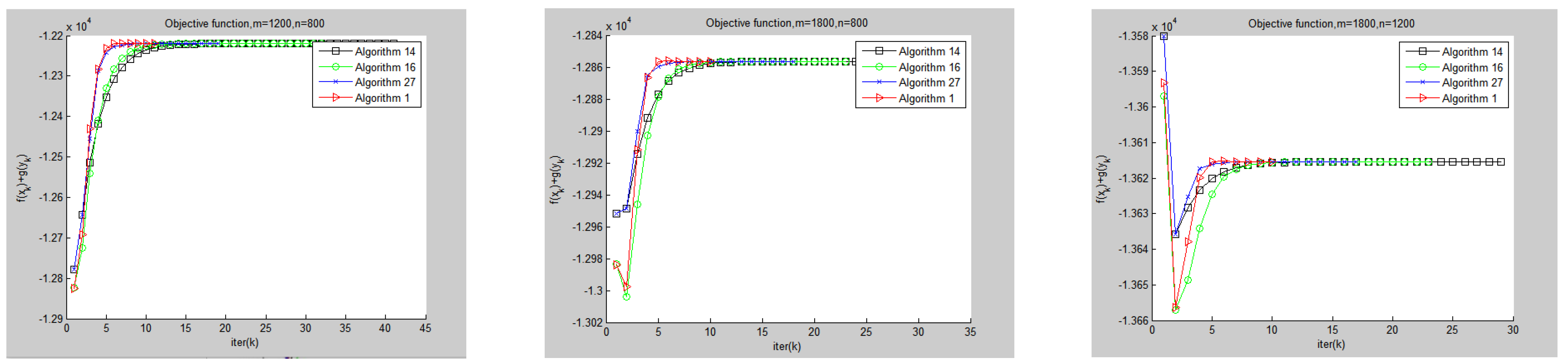
3. Numerical Experiments

In this section, some numerical experiments will be tested to illustrate the efficiency of Algorithm 1. The experiments are divided into two parts. In the first part, we first analyze the relationship between the parameters r and s and the convergence of Algorithm 1 and give the selection range of the best parameters r and s. Then, we give a comparison of Algorithm 1 with the algorithm proposed in [15], the algorithm proposed in [16], and the algorithm proposed in [27] to solve a convex quadratic programming problem. In the second part, we give the numerical comparison between Algorithm 1 and the algorithm proposed in [16] in image restoration. All codes were written in MATLAB R2019a, and all experiments were performed on a personal computer with an Intel(R) Core i7-6567U processor (3.3 GHz) and 8 GB memory.

3.1. Convex Quadratic Programming Problem

To specify the problem (Equation (1)), we choose a separable convex quadratic programming problem proposed in [31], where

$$f\left(x\right)={\displaystyle \frac{1}{2}}{x}^T{M}_{1}x+q_1{}^{T}x\mathrm{and}g\left(y\right)={\displaystyle \frac{1}{2}}{y}^T{M}_{2}y+q_2{}^{T}y,$$

and here the matrices $M_i=Q_i^T{Q}_i(i=1,2)$, and $Q_1\in {ℝ}^{m\times m}$, and $Q_2\in {ℝ}^{n\times n}$ are randomly generated square matrices with all entries are chosen in intervals [−5, 5]. The vectors $q_i(i=1,2)$ are generated from a uniform distribution in the interval [−500, 500]. For the linear constraint, $A=1_{1\times m}$ and $B=1_{1\times n}$ (i.e., all entries of A and B are taken as 1), and $b=\left(m+n\right)/100$. The convex set $\mathcal{X}\subset {ℝ}^m$ is defined as a sphere with the origin at the center of the circle and radius $r=1$, and the convex set $\mathcal{Y}\subset {ℝ}^n$ is defined as the box in ${ℝ}^n$ with all entries are chosen in intervals [0, 5].

Since the convergence of the original ADMM algorithm is well proven, the algorithm proposed in [11] may not converge in some cases, the symmetric ADMM algorithm proposed in [16] has a larger step size relative to the algorithm in [16], and the adaptive penalty parameter has been less studied. Therefore, we only compare Algorithm 1 numerically with the algorithms presented in references [14], [16] and [27] denoted respectively by Algorithm 14, 16 and 27.

To ensure the fairness of the experiment, the parameter $\gamma$ of Algorithm 14 and 27 is chosen as the optimal value $\gamma =1.6$; the parameters r and s of the algorithm proposed in [18] are chosen as the optimal value r = 0.8, s = 1.17; and the initial penalty parameter $\beta$ of all algorithms mentioned above is chosen as 1. The initial iterations for all tested methods are zero vectors, and the stopping criterion is chosen as

$$\max \left\{{‖A{x}_{k+1}+B{y}_{k+1}-b‖}_2,{‖B{y}_k-B{y}_{k+1}‖}_2\right\}\le \epsilon ={10}^{-6}$$

For Algorithm 1, we take

$${\tau }_k=\left\{\begin{array}{l}0.3,ifk\le k_{\max },\\ 0,otherwise.\end{array}\right.$$

The parameters of Algorithm 2, which solves the x-subproblem and the y-subproblem of Algorithm 1, are chosen as $\theta =0.1$, $\nu =0.8$, and $\mathcal{l}=1.8$. Table 1 reports the iteration numbers (Iter) and computation time (Time) of Algorithm 1 with different parameters r and s, and the best estimate of the parameters r and s can be chosen as r = 0.95, s = 1.12. And so, in the following numerical comparison experiment, the parameters r and s of Algorithm 1 are chosen as r = 0.95, s = 1.12.

Table 1. The numerical comparison of Algorithm 1 with different parameters r and s.

m	n	r = 0.95 s = 1.12		r = 0.9 s = 1		r = s = 1		r = 1 s = 1.5		r = 1.54 s = 0.2		r = 0.1 s = 1.57
		Iter	Time	Iter	Time	Iter	Time	Iter	Time	Iter	Time	Iter	Time
800	200	10.7	0.41	11.4	0.44	10.8	0.44	11.1	0.46	17.7	0.65	19.1	0.71
600	400	10.7	0.26	11.4	0.29	11.0	0.27	11.6	0.29	16.6	0.42	18.7	0.49
1600	400	10.0	1.51	10.3	1.66	9.9	1.61	11.0	1.75	18.5	2.84	18.0	2.82
1200	800	10.0	1.13	10.7	1.26	9.9	1.16	10.7	1.27	17.8	2.05	18.0	2.08
2400	600	9.7	6.95	10.1	7.23	9.7	6.98	10.8	7.72	19.0	13.13	17.1	12.30
1800	1200	9.6	2.73	10.3	3.06	9.8	2.92	11.2	3.30	18.2	5.22	17.0	5.03
3200	800	9.8	15.32	10.0	15.59	10.1	15.81	10.3	16.01	19.0	29.22	16.8	26.24
2400	1600	9.7	8.54	10.1	8.83	10.2	8.83	10.8	9.34	17.1	14.30	15.6	13.86

In Table 2, we show the iteration numbers (Iter), the computational time (Time) of Algorithm 1, and Algorithm14, 16 and 27 for solving the separable convex quadratic programming problem proposed in [31]. To investigate the stability and accuracy of the algorithms, we tested 8 different sets of m and n values throughout the experiment, running each set of data 10 times and averaging the final results. In Figure 1, we plot the comparison in terms of objective function values (Obj) and computing time with Algorithm 1, and Algorithm14, Algorithm16 and Algorithm27 for solving the separable convex quadratic programming problem proposed in [31].

Table 2. The numerical comparison of Algorithm 1 with the other three algorithms.

m	n	obj	Algorithm 1		Algorithm 16		Algorithm 27		Algorithm 14
			r = 0.95, s = 1.12		r = 0.8, s = 1.17		$\mathit{\gamma }=1.6$		$\mathit{\gamma }=1.6$
			Iter	Time	Iter	Time	Iter	Time	Iter	Time
800	200	−9478.39	10.6	0.41	39.1	1.41	20.2	0.68	50.1	1.79
600	400	−8939.27	10.7	0.26	42.4	1.19	20.0	0.51	54.1	1.47
1600	400	−12,473.27	10.0	1.51	29.1	5.13	18.9	3.06	37.5	6.62
1200	800	−12,038.11	10.0	1.13	30.1	3.77	19.0	2.16	38.8	4.84
2400	600	−14,789.51	9.5	6.95	21.7	15.56	17.6	12.61	27.9	20.01
1800	1200	−14,312.39	9.8	2.73	22.9	7.19	18.0	5.30	30.1	9.51
3200	800	−16,191.25	9.8	15.32	18.3	28.18	17.3	27.32	23.8	36.43
2400	1600	−14,365.07	9.7	8.54	19.7	17.03	17.3	14.99	25.5	21.98

Figure 1. Objective function curve of Algorithm 1 and the other three algorithms.

Based on the tests reported in Table 2, Figure 1, and many other performed unreported tests that show similar patterns, we know that Algorithm 1 is more efficient than other existing algorithms.

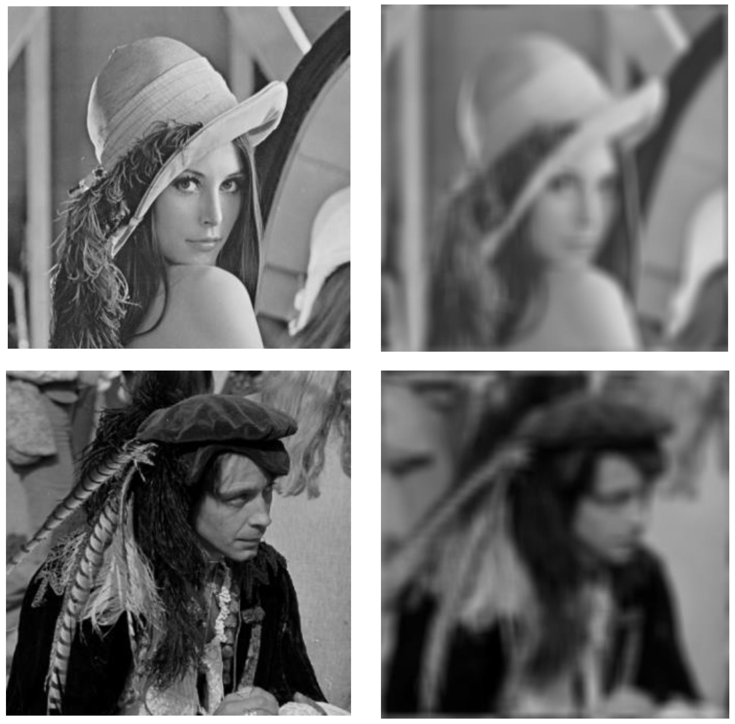
3.2. Image Restoration Problem

In this subsection, we consider the total variational image deblurring model proposed in [16], whose discretized version can be written as

$$\underset{y}{\min }{‖Ay‖}_1+\frac{\lambda }{2}{‖Bx-z‖}^2$$

(34)

where $y\in {\mathcal{R}}^n$ represents a digital clean image, $z\in {\mathcal{R}}^n$ is a corrupted input image, $A:=\left({\partial }_1,{\partial }_2\right):{\mathcal{R}}^n\to {\mathcal{R}}^n\times {\mathcal{R}}^n$ is the discrete gradient operator, and ${\partial }_1:{\mathcal{R}}^n\to {\mathcal{R}}^n$ and ${\partial }_2:{\mathcal{R}}^n\to {\mathcal{R}}^n$ are the discrete derivatives in the horizontal and vertical directions, respectively.$B:{\mathcal{R}}^n\to {\mathcal{R}}^n$ is the matrix representation of a spatially invariant blurring operator, λ > 0 is a constant balancing the data fidelity and total variational regularization terms, and ${‖\cdot ‖}_1$ defined on ${\mathcal{R}}^n\times {\mathcal{R}}^n$ is given by

$${‖x‖}_1={\displaystyle \sum _{\{i,j\}=1}^n\sqrt{{\left|x_{i,j}^1\right|}^2+{\left|x_{i,j}^2\right|}^2}},\forall x=(x^1,x^2)\in {\mathcal{R}}^n\times {\mathcal{R}}^n,$$

This is a basic model for various more advanced image processing tasks, and it has been studied extensively in the literature. Introducing the auxiliary variable x, we can reformulate Equation (34) as

$$\underset{x,y}{\min }{‖x‖}_1+\frac{\lambda }{2}{‖By-z‖}^2\mathrm{s}.\mathrm{t}x-Ay=0$$

which is a special case of the generic model (Equation (1)) under discussion, and thus Algorithm 1 is applicable.

We test two images lena.tif (512 × 512) and man.pgm (512 × 512). These images are first corrupted by the blur operator with kernel size of 21 × 21, and then the blurred images are further corrupted by zero-white Gaussian noise with a standard derivation 0.002. In Figure 2, we list the original and degraded images. The quality of restored images is measured by the value of the SNR given by

$$\mathrm{SNR}=20{\log }_{10}{\displaystyle \frac{‖y‖}{‖y-\overline{y}‖}}$$

where $y$ is the original image and $\overline{y}$ is the recovered image. A larger SNR value means a higher quality of the restored image. Table 3 and Figure 3 report the comparison experiment between Algorithm 1 and the algorithm proposed in [16] for the image restoration problem.

Figure 2. First column is original images; second column is corrupted images.

Table 3. The numerical comparison of Algorithm 1 and the algorithm in [16].

	Lena (512 × 512)			man (512 × 512)
	Iter	Time	SNR	Iter	Time	SNR
Algorithm 1 r = 0.95, s = 1.12	26	3.93	23.02	30	4.51	17.02
Algorithm 16 r =0.8, s = 1.17	37	5.54	23.00	40	6.08	17.00

Figure 3. First column is blurred images; second column is recovered images by Algorithm 1; and third column is recovered images by the algorithm in [18].

4. Conclusions

The alternating direction method is one of the most attractive approaches for solving convex optimization problems with linear constraints and separable objective functions. Experience with applications has shown that the iteration numbers and computing time depend significantly on the penalty parameter for the linear constraint. The penalty parameters in the classical alternating direction method are a constant. In this paper, we, based on the idea of references [16,28], propose an adaptive penalty parameter alternate direction method of multipliers with attach relaxation factors and with the Lagrange multiplier updated twice at each iteration (Algorithm 1), which not only adaptively adjusts the penalty parameters per iteration based on the iteration message but also adds relaxation factors to the Lagrange multiplier update steps. For the proposed algorithm, that is, Algorithm 1, the global convergence is proven (that is, Theorem 1). Preliminary numerical experiments show that the technique of adaptive adjusting of penalty parameters per iteration and attaching relaxation factors in Lagrange multiplier updating steps are effective in practical applications (see Table 2 and Figure 1).

References

- Yang, J.F.; Zhang, Y. Alternating direction algorithms for l1-problems in compressive sensing. SIAM J. Sci. Comput. 2011, 33, 250–278. [Google Scholar] [CrossRef]
- Li, J.C. A parameterized proximal point algorithm for separable convex optimization. Optim. Lett. 2018, 12, 1589–1608. [Google Scholar]
- Tao, M.; Yuan, X.M. Recovering low-rank and sparse components of matrices from incomplete and noisy observations. SIAM J. Optim. 2011, 21, 57–81. [Google Scholar] [CrossRef]
- Hager, W.W.; Zhang, H.C. Convergence rates for an inexact ADMM applied to separable convex optimization. Comput. Optim. Appl. 2020, 77, 729–754. [Google Scholar] [CrossRef]
- Liu, Z.S.; Li, J.C.; Liu, X.N. A new model for sparse and Low-Rank matrix decomposition. J. Appl. Anal. Comput. 2017, 7, 600–616. [Google Scholar]
- Jiang, F.; Wu, Z.M. An inexact symmetric ADMM algorithm with indefinite proximal term for sparse signal recovery and image restoration problems. J. Comput. Appl. Math. 2023, 417, 114628. [Google Scholar] [CrossRef]
- Bai, J.C.; Hager, W.W.; Zhan, H.C. An inexact accelerated stochastic ADMM for separable convex optimization. Comput. Optim. Appl. 2022, 81, 479–518. [Google Scholar] [CrossRef]
- Boyd, S.; Parikh, N.; Chu, E.; Peleato, B.; Eckstein, J. Distributed optimization and statistical learning via the alternation direction method of multipliers. Found. Trends Mach. Learn. 2011, 3, 1–122. [Google Scholar] [CrossRef]
- Chan, T.F.; Glowinski, R. Finite Element Approximation and Iterative Solution of a Class of Mildly Nonlinear Elliptic Equations; Technical Report STAN-CS-78-674; Computer Science Department, Stanford University: Stanford, CA, USA, 1978. [Google Scholar]
- Hestenes, M.R. Multiplier and gradient methods. J. Optim. Theory Appl. 1969, 4, 303–320. [Google Scholar] [CrossRef]
- Lions, P.L.; Mercier, B. Splitting algorithms for the sum of two nonlinear operators. SIAM J. Numer. Anal. 1979, 16, 964–979. [Google Scholar] [CrossRef]
- Cai; X. J.; Gu, G.Y.; He, B.S.; Yuan, X.M. A proximal point algorithm revisit on the alternating direction method of multipliers. Sci. China Math. 2013, 56, 2179–2186. [Google Scholar] [CrossRef]
- Fortin, M.; Glowinski, R. Augmented Lagrangian Methods: Applications to the Numerical Solution of Boundary-Value Problems; North-Holland: Amsterdam, The Netherlands, 1983. [Google Scholar]
- Glowinski, R.; Karkkainen, T.; Majava, K. On the Convergence of Operator-Splitting Methods, in Numerical Methods for Scientific Computing, Variational Problems and Applications; Heikkola, E., Kuznetsov, P.Y., Neittaanm, P., Pironneau, O., Eds.; CIMNE: Barcelona, Spain, 2003; pp. 67–79. [Google Scholar]
- He, B.S.; Liu, H.; Wang, Z.R.; Yuan, X.M. A strictly contractive Peaceman-Rachford splitting method for convex programming. SIAM J. Optim. 2014, 24, 1011–1040. [Google Scholar] [CrossRef] [PubMed]
- He, B.S.; Ma, F.; Yuan, X.M. Convergence study on the symmetric version of ADMM with larger step sizes. SIAM J. Imaging Sci. 2016, 9, 1467–1501. [Google Scholar] [CrossRef]
- Luo, G.; Yang, Q.Z. A fast symmetric alternating direction method of multipliers. Numer. Math. Theory Meth. Appl. 2020, 13, 200–219. [Google Scholar]
- Li, X.X.; Yuan, X.M. A proximal strictly contractive Peaceman-Rachford splitting method for convex programming with applications to imaging. SIAM J. Imaging Sci. 2015, 8, 1332–1365. [Google Scholar] [CrossRef]
- Bai, J.C.; Li, J.C.; Xu, F.M.; Zhang, H.C. Generalized symmetric ADMM for separable convex optimization. Comput. Optim. Appl. 2018, 70, 129–170. [Google Scholar] [CrossRef]
- Wu, Z.M.; Li, M. An LQP-based symmetric Alternating direction method of multipliers with larger step sizes. J. Oper. Res. Soc. China 2019, 7, 365–383. [Google Scholar] [CrossRef]
- Chang, X.K.; Bai, J.C.; Song, D.J.; Liu, S.Y. Linearized symmetric multi-block ADMM with indefinite proximal regularization and optimal proximal parameter. Calcolo 2020, 57, 38. [Google Scholar] [CrossRef]
- Han, D.R.; Sun, D.F.; Zhang, L.W. Linear rate convergence of the alternating direction method of multipliers for convex composite programming. Math. Oper. Res. 2018, 43, 622–637. [Google Scholar] [CrossRef]
- Gao, B.; Ma, F. Symmetric alternating direction method with indefinite proximal regularization for linearly constrained convex optimization. J. Optim. Theory Appl. 2018, 176, 178–204. [Google Scholar] [CrossRef]
- Shen, Y.; Zuo, Y.N.; Yu, A.L. A partially proximal S-ADMM for separable convex optimization with linear constraints. Appl. Numer. Math. 2021, 160, 65–83. [Google Scholar] [CrossRef]
- Adona, V.A.; Goncalves, M.L.N. An inexact version of the symmetric proximal ADMM for solving separable convex optimization. Numer. Algor. 2023, 94, 1–28. [Google Scholar] [CrossRef]
- He, B.S.; Yang, H. Some convergence properties of a method of multipliers for linearly constrained monotone variational inequalities. Oper. Res. Lett. 1998, 23, 151–161. [Google Scholar] [CrossRef]
- He, B.S.; Yang, H.; Wang, S.L. Alternating direction method with Self-Adaptive penalty parameters for monotone variational inequalities. J. Optim. Theory Appl. 2000, 106, 337–356. [Google Scholar] [CrossRef]
- He, B.S.; Liao, L.Z. Improvements of some projection methods for monotone nonlinear variational inequalities. J. Optim. Theory Appl. 2002, 112, 111–128. [Google Scholar] [CrossRef]
- Palomar, D.P.; Scutari, G. Variational inequality theory a mathematical framework for multiuser communication systems and signal processing. In Proceedings of the International Workshop on Mathematical of Issues in Information Sciences-MIIS, Xi’an, China, 7–13 July 2012. [Google Scholar]
- He, B.S. A new method for a class of linear variational inequalities. Math. Programm. 1994, 66, 137–144. [Google Scholar] [CrossRef]
- Han, D.R.; He, H.J.; Yang, H.; Yuan, X.M. A customized Douglas–Rachford splitting algorithm for separable convex minimization with linear constraints. Numer. Math. 2014, 127, 167–200. [Google Scholar] [CrossRef]
Disclaimer/Publisher’s Note: The statements, opinions and data contained in all publications are solely those of the individual author(s) and contributor(s) and not of MDPI and/or the editor(s). MDPI and/or the editor(s) disclaim responsibility for any injury to people or property resulting from any ideas, methods, instructions or products referred to in the content. |
© 2025 by the authors. Licensee MDPI, Basel, Switzerland. This article is an open access article distributed under the terms and conditions of the Creative Commons Attribution (CC BY) license (https://creativecommons.org/licenses/by/4.0/).