
Structural Properties of Optimal Maintenance Policies for k-out-of-n Systems with Interdependence Between Internal Deterioration and External Shocks †


Abstract
1. Introduction
- We propose an optimal maintenance policy for k-out-of-n systems that accounts for variability in shock impacts across units and addresses the interdependence between unit deterioration and external shocks, making it applicable to real-world systems for efficient operation.
- We derive a structural property of the optimal policy, offering key insights for developing algorithms that enable efficient searching for the optimal solution.

| System Design | Interdependence Among Units | Interdependence Between External Shocks and Internal Deterioration | Optimization Target | Optimization Framework | Structural Property | |
|---|---|---|---|---|---|---|
| Derman [3] | single-unit | - | - | maintenance action | MDP | ✓ |
| Ohnishi et al. [4] | single-unit | - | - | maintenance action | partially observable MDP | ✓ |
| Lovejoy et al. [5] | single-unit | - | - | maintenance action | partially observable MDP | ✓ |
| Elwany et al. [6] | single-unit | - | - | maintenance action | MDP | ✓ |
| Chen et al. [7] | single-unit | - | - | maintenance action | MDP | ✓ |
| Zhu and Xiang [11] | n-unit | × | - | maintenance action | stochastic programming | ✓ |
| Ashizawa and Jin [13] | 2-unit | ✓ | - | maintenance action | MDP | ✓ |
| Liu et al. [14] | series | ✓ | - | maintenance action | MDP | ✓ |
| Xu et al. [16] | k-out-of-n | ✓ | - | maintenance action | MDP | - |
| Oakley et al. [17] | series–parallel | ✓ | - | maintenance action | Bayesian sequential decision | ✓ |
| Sun et al. [18] | k-out-of-n | × | - | maintenance action | MDP | ✓ |
| Zhang et al. [19] | k-out-of-n | ✓ | - | maintenance action | MDP | ✓ |
| Rafiee et al. [24] | single-unit | - | × | inspection interval | cost rate | - |
| Dui et al. [25] | n-unit | × | age→internal deterioration age→shocks | maintenance action | integer programming | - |
| Yousefi et al. [26] | series parallel | × | × | maintenance action | MDP | - |
| Yousefi et al. [27] | series | × | internal deterioration ↔ external shocks | inspection interval | cost rate | - |
| Tajiani [28] | single-unit | - | internal deterioration ← external shocks | maintenance threshold | cost rate | - |
| Kurt and Maillart [29] | single-unit | - | internal deterioration ← external shocks | maintenance action | MDP | ✓ |
| Wang et al. [30] | single-unit | - | internal deterioration ↔ external shocks | maintenance action | MDP | ✓ |
| Qi and Huang et al. [31] | single-unit | - | internal deterioration ↔ external shocks | inspection interval | cost rate | - |
| Lorvand and Kelkinnama. [33] | k-out-of-n | × | age→external shocks | maintenance interval | cost rate | - |
| Cao et al. [39] | single-unit | - | internal deterioration ← external shocks age→external shocks | inspection interval | multi objective programming | - |
| Shafiee et al. [40] | series | × | - | maintenance threshold maintenance interval | cost rate | - |
| This research | k-out-of-n | ✓ | internal deterioration ↔ external shocks | maintenance action | MDP | ✓ |
2. Model
2.1. System Deterioration
2.2. Actions and Costs in Condition-Based Maintenance
2.3. Optimal Maintenance Policy
3. Structural Properties of the Optimal Maintenance Policy
- 1.
- Base Case : By Equation (1) and Assumption 1, holds. Since each unit’s deterioration is independent of other unit deterioration states, it follows from Lemma 2 that .
- 2.
- Inductive Step: Assume that holds for all when .
4. Case Study: Three-Bladed Rotor System of Offshore Wind Turbines
4.1. System and Parameter Specifications
4.2. Optimal Maintenance Policy for a Three-Bladed Rotor System of Offshore Wind Turbines
| Algorithm 1 The value iteration algorithm utilized to compute . |
|
4.3. Performance of the Proposed Policy
| Algorithm 2 Calculate average total discounted cost and availability for each policy. |
|
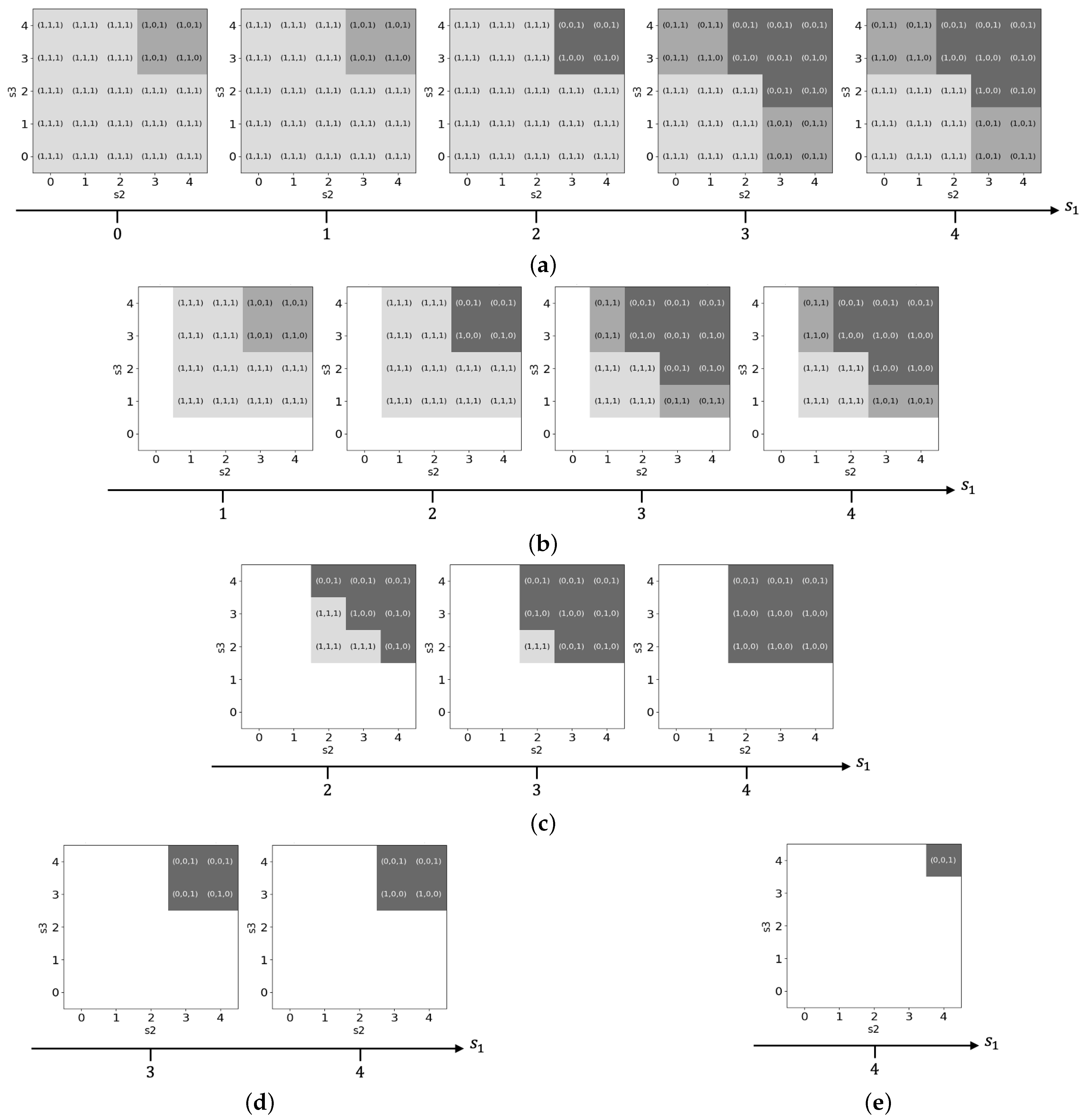
4.4. The 2-out-of-3 System
5. Sensitivity Analysis
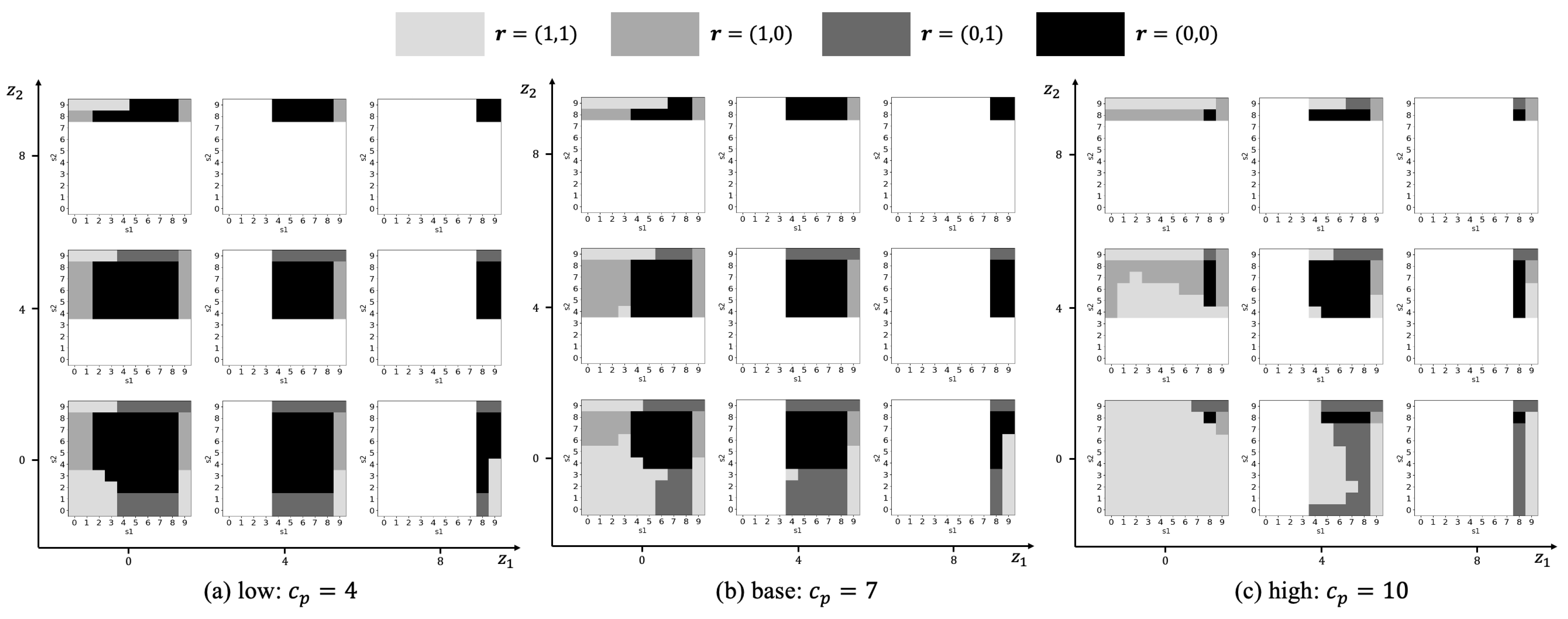
5.1. Preventive Replacement Cost ()
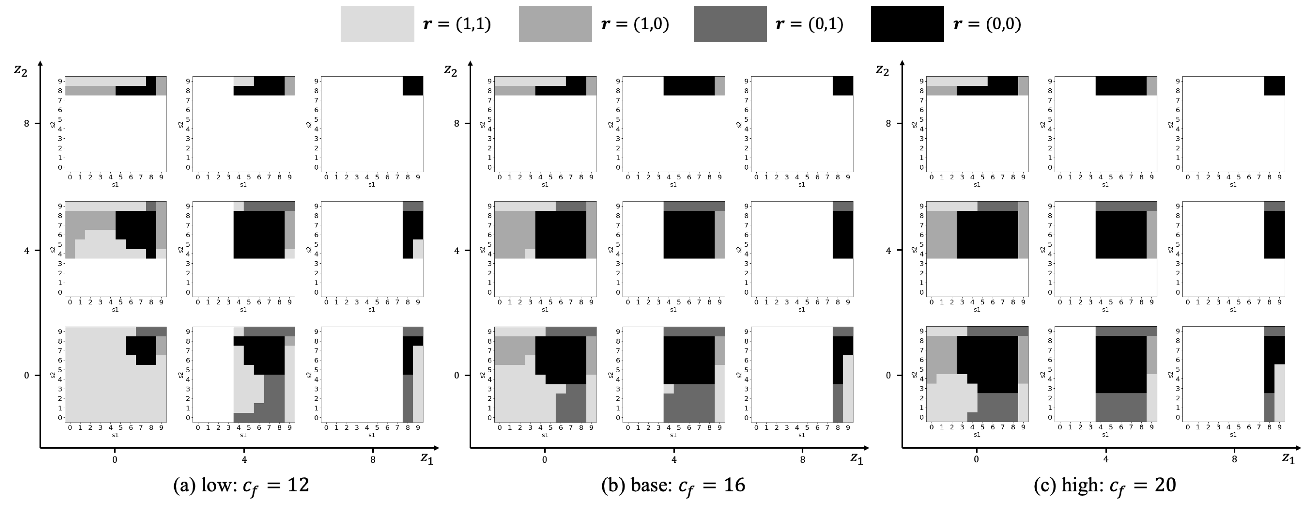
5.2. Corrective Replacement Cost ()
5.3. Downtime Cost ()

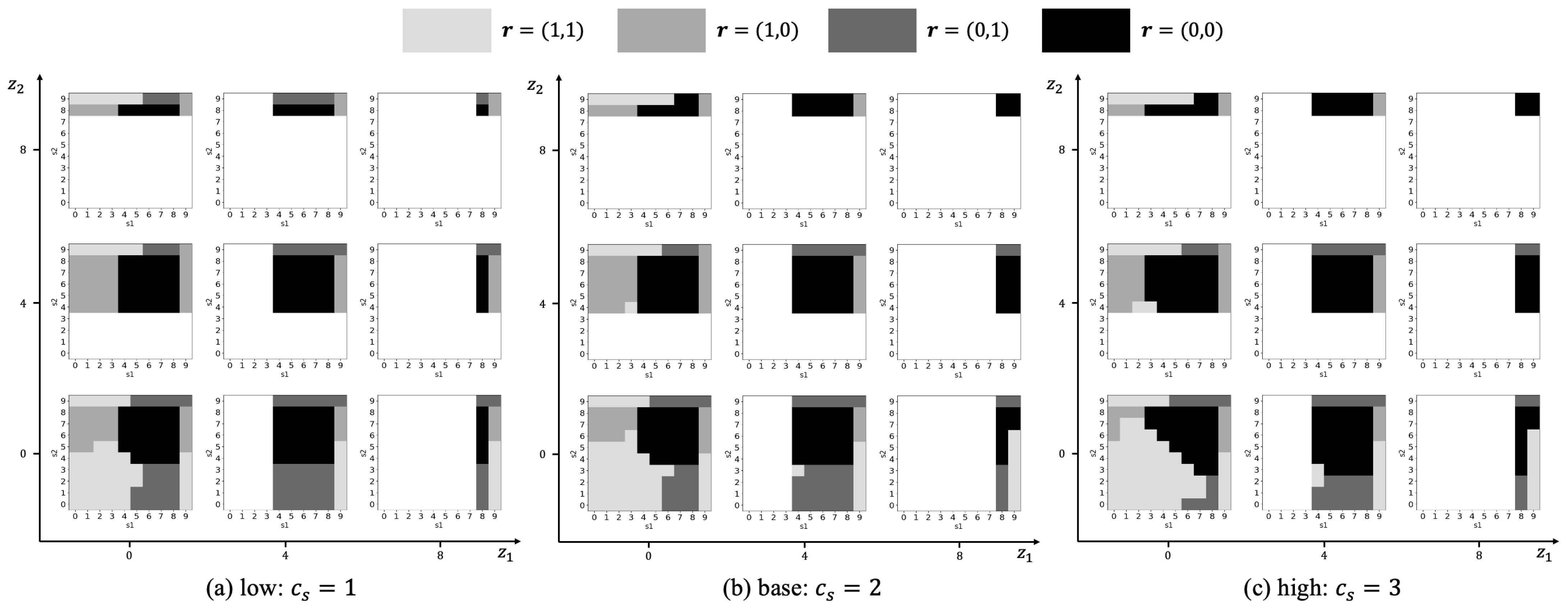
5.4. Setup Cost ()
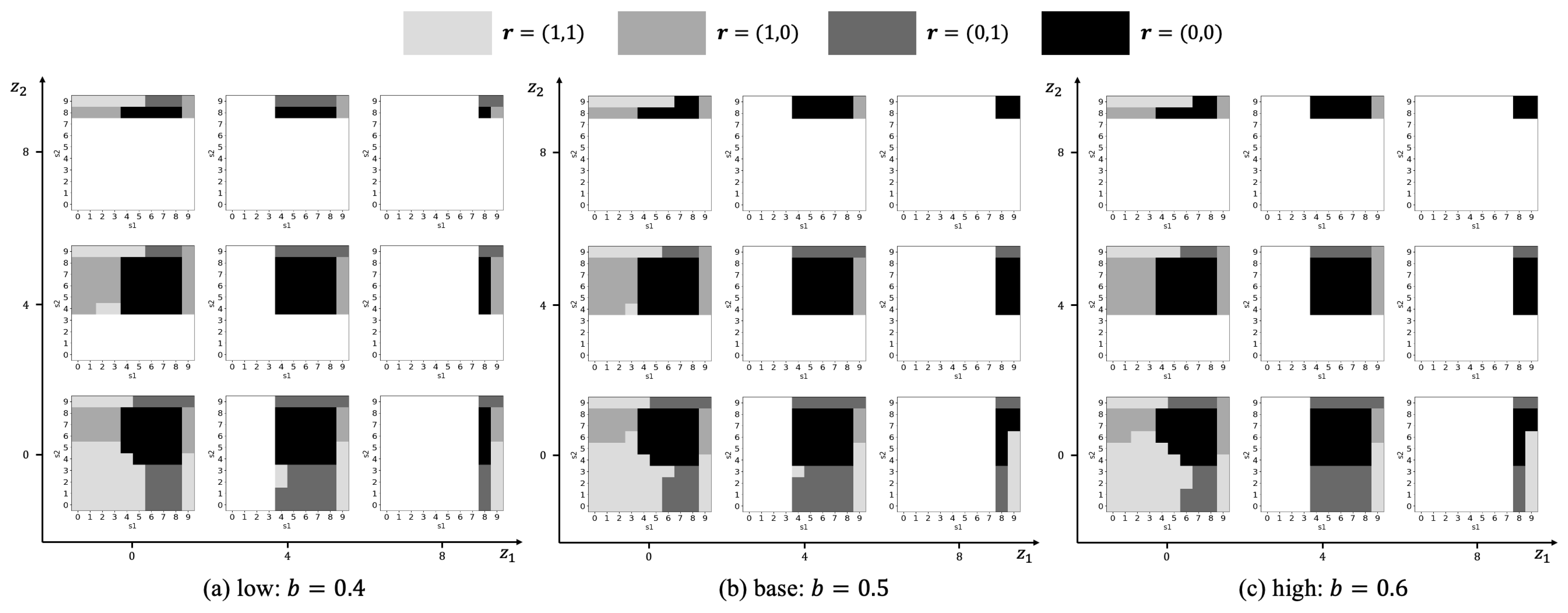
5.5. Coefficient in Scale Parameter Model (b)
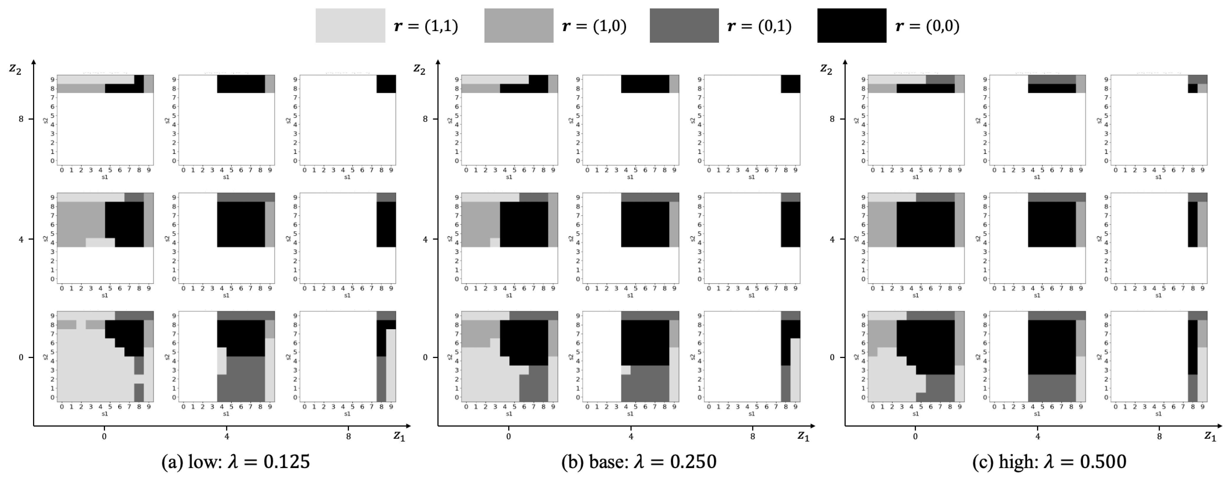
5.6. Shock Likelihood ()
6. Conclusions
Author Contributions
Funding
Data Availability Statement
Conflicts of Interest
Nomenclature
| Fixed inspection interval | |
| Deterioration state of unit i | |
| Deterioration state of system | |
| Shock-induced cumulative deterioration of unit i | |
| Shock-induced cumulative deterioration of system | |
| L | Failure threshold of units |
| Elapsed time from last inspection to system failure | |
| Shape parameter of units | |
| Scale parameter of unit i given | |
| Expected down time cost given and | |
| Constant preventive replacement cost | |
| Constant corrective replacement cost | |
| Constant setup cost | |
| Constant downtime cost | |
| Discount factor | |
| Shock type | |
| Set of units whose deterioration state increases due to shocks of type m | |
| Transition probability density function from to given after time t | |
| Probability density function that type m shock occurs at time t | |
| Probability density function that the increment of unit deterioration is when a shock of type m occurs in unit i |
References
- Alaswad, S.; Xiang, Y. A review on condition-based maintenance optimization models for stochastically deteriorating system. Reliab. Eng. Syst. Saf. 2017, 157, 54–63. [Google Scholar] [CrossRef]
- Li, Y.; Peng, S.; Li, Y.; Jiang, W. A review of condition-based maintenance: Its prognostic and operational aspects. Front. Eng. Manag. 2020, 7, 323–334. [Google Scholar] [CrossRef]
- Derman, C. On optimal replacement rules when changes of state are Markovian. Math. Optim. Tech. 1963, 396, 201–210. [Google Scholar]
- Ohnishi, M.; Kawai, H.; Mine, H. An optimal inspection and replacement policy under incomplete state information. Eur. J. Oper. Res. 1986, 27, 117–128. [Google Scholar] [CrossRef]
- Lovejoy, M.S. Some monotonicity results for partially observed Markov decision processes. Oper. Res. 1987, 35, 736–743. [Google Scholar] [CrossRef]
- Elwany, A.H.; Gebraeel, N.Z.; Maillart, L.M. Structured replacement policies for components with complex degradation processes and dedicated sensors. Oper. Res. 2011, 59, 684–695. [Google Scholar] [CrossRef]
- Chen, N.; Ye, Z.; Xiang, Y.; Zhang, L. Condition-based maintenance using the inverse Gaussian degradation model. Eur. J. Oper. Res. 2015, 243, 190–199. [Google Scholar] [CrossRef]
- Keizer, M.C.O.; Flapper, S.D.P.; Teunter, R.H. Condition-based maintenance policies for systems with multiple dependent components: A review. Eur. J. Oper. Res. 2017, 261, 405–420. [Google Scholar] [CrossRef]
- Kobbacy, K.A.; Murthy, D.P.; Nicolai, R.P.; Dekker, R. Optimal Maintenance of Multi-Component Systems: A Review; Springer: London, UK, 2008; pp. 263–286. [Google Scholar]
- Bellman, R.E. Dynamic Programming; Princeton University Press: Princeton, NJ, USA, 1957. [Google Scholar]
- Zhu, Z.; Xiang, Y. Condition-based maintenance for multi-component systems: Modeling, structural properties, and algorithms. IISE Trans. 2021, 53, 88–100. [Google Scholar] [CrossRef]
- Chen, J.; Kim, M.H. Review of recent offshore wind turbine research and optimization methodologies in their design. J. Mar. Sci. Eng. 2022, 10, 28. [Google Scholar] [CrossRef]
- Ashizawa, R.; Jin, L. Joint maintenance and load-sharing optimization for two-unit systems with workload-dependent deterioration. Total Qual. Sci. 2022, 8, 40–50. [Google Scholar] [CrossRef]
- Liu, B.; Pandey, M.D.; Wang, X.; Zhao, X. A finite-horizon condition-based maintenance policy for a two-unit system with dependent degradation processes. Eur. J. Oper. Res. 2021, 295, 705–717. [Google Scholar] [CrossRef]
- Krishnamoorthy, A. Analysis of reliability of interdependent serial, parallel and the general k-out-of-n: G system: A new approach. J. Indian Soc. Probab. Stat. 2022, 23, 483–496. [Google Scholar] [CrossRef]
- Xu, J.; Liang, Z.; Li, Y.; Wang, K. Generalized condition-based maintenance optimization for multi-component systems considering stochastic dependency and imperfect maintenance. Reliab. Eng. Syst. Saf. 2021, 211, 107592. [Google Scholar] [CrossRef]
- Oakley, J.L.; Wilson, K.J.; Philipson, P. A condition-based maintenance policy for continuously monitored multi-component systems with economic and stochastic dependence. Reliab. Eng. Syst. Saf. 2022, 222, 108321. [Google Scholar] [CrossRef]
- Sun, Q.; Ye, Z.; Chen, N. Optimal inspection and replacement policies for multi-unit systems subject to deterioration. IEEE Trans. Reliab. 2017, 67, 401–413. [Google Scholar] [CrossRef]
- Zhang, N.; Tian, S.; Cai, K.; Zhang, J. Condition-based maintenance assessment for a deteriorating system considering stochastic failure dependence. IISE Trans. 2023, 55, 687–697. [Google Scholar] [CrossRef]
- Ahmad, R.; Kamaruddin, S. An overview of time-based and condition-based maintenance in industrial application. Comput. Ind. Eng. 2012, 63, 135–149. [Google Scholar] [CrossRef]
- Dui, H.; Lu, Y.; Wu, S. Competing risks-based resilience approach for multi-state systems under multiple shocks. Reliab. Eng. Syst. Saf. 2024, 242, 109773. [Google Scholar] [CrossRef]
- Zhao, X.; Sun, L.; Wang, M.; Wang, X. A shock model for multi-component system considering the cumulative effect of severely damaged components. Comput. Ind. Eng. 2019, 137, 106027. [Google Scholar] [CrossRef]
- Katsaprakakis, D.A.; Papadakis, N.; Ntintakis, I. A comprehensive analysis of wind turbine blade damage. Energies 2021, 14, 5974. [Google Scholar] [CrossRef]
- Rafiee, K.; Feng, Q.; Coit, D.W. Condition-based maintenance for repairable deteriorating systems subject to a generalized mixed shock model. IEEE Trans. Reliab. 2015, 64, 1164–1174. [Google Scholar] [CrossRef]
- Dui, H.; Zhang, H.; Wu, S. Optimisation of maintenance policies for a deteriorating multi-component system under external shocks. Reliab. Eng. Syst. Saf. 2023, 238, 109415. [Google Scholar] [CrossRef]
- Yousefi, N.; Tsianikas, S.; Coit, D.W. Dynamic maintenance model for a repairable multi-component system using deep reinforcement learning. Qual. Eng. 2022, 34, 16–35. [Google Scholar] [CrossRef]
- Yousefi, N.; Coit, D.W.; Zhu, X. Dynamic maintenance policy for systems with repairable components subject to mutually dependent competing failure processes. Comput. Ind. Eng. 2020, 143, 106398. [Google Scholar] [CrossRef]
- Tajiani, B.; Vatn, J.; Naseri, M. Optimizing the maintenance threshold in presence of shocks: A numerical framework for systems with non-monotonic degradation. Reliab. Eng. Syst. Saf. 2024, 245, 110039. [Google Scholar] [CrossRef]
- Kurt, M.; Maillart, L.M. Structured replacement policies for a Markov-modulated shock model. Oper. Res. Lett. 2009, 37, 280–284. [Google Scholar] [CrossRef]
- Wang, Z.; Jin, L.; Yamamoto, W. Optimal maintenance policy for deteriorating systems subject to external shock damage under a semi-Markov decision process. Total Qual. Sci. 2023, 9, 83–97. [Google Scholar]
- Qi, F.; Huang, M. Optimal condition-based maintenance policy for systems with mutually dependent competing failure. Qual. Reliab. Eng. Int. 2023, 39, 1831–1847. [Google Scholar] [CrossRef]
- Dong, W.; Liu, S.; Bae, S.J.; Cao, Y. Reliability modelling for multi-component systems subject to stochastic deterioration and generalized cumulative shock damages. Reliab. Eng. Syst. Saf. 2021, 205, 107260. [Google Scholar] [CrossRef]
- Lorvand, H.; Kelkinnama, M. Reliability analysis and optimal replacement for a k-out-of-n system under a δ-shock model. Proc. Inst. Mech. Eng. Part O J. Risk Reliab. 2023, 237, 98–111. [Google Scholar] [CrossRef]
- Shen, J.; Elwany, A.; Cui, L. Reliability analysis for multi-component systems with degradation interaction and categorized shocks. Appl. Math. Model. 2018, 56, 487–500. [Google Scholar] [CrossRef]
- Wang, X.; Zhao, X.; Zhao, X.; Chen, X.; Ning, R. Reliability assessment for a generalized k-out-of-n: F system under a mixed shock model with multiple sources. Comput. Ind. Eng. 2024, 196, 110459. [Google Scholar] [CrossRef]
- Wang, X.; Zhao, X.; Wu, C.; Wang, S. Mixed shock model for multi-state weighted k-out-of-n: F systems with degraded resistance against shocks. Reliab. Eng. Syst. Saf. 2022, 217, 108098. [Google Scholar] [CrossRef]
- Huang, X.; Xu, L.; Huang, Y.; Fang, Y. Reliability analysis for k-out-of-n: F load sharing systems operating in a shock environment. IEEE Access 2023, 11, 18227–18233. [Google Scholar] [CrossRef]
- Kasuya, M.; Jin, L. Maintenance policy for deteriorating k-out-of-n systems subject to random shocks. In Proceedings of the 11th Asia-Pacific International Symposium on Advanced Reliability and Maintenance Modeling (APARM2024), Nagoya City, Japan, 26–30 August 2024. [Google Scholar]
- Cao, Y.; Luo, J.; Dong, W. Optimization of condition-based maintenance for multi-state deterioration systems under random shock. Appl. Math. Model. 2023, 115, 80–99. [Google Scholar] [CrossRef]
- Shafiee, M.; Finkelstein, M.; Berenguer, C. An opportunistic condition-based maintenance policy for offshore wind turbine blades subjected to degradation and environmental shocks. Reliab. Eng. Syst. Saf. 2015, 142, 463–471. [Google Scholar] [CrossRef]
- Van Noortwijk, J.M. A survey of the application of gamma processes in maintenance. Reliab. Eng. Syst. Saf. 2009, 94, 2–21. [Google Scholar] [CrossRef]
- Puterman, M. Markov Decision Processes: Discrete Stochastic Dynamic Programming; John Wiley & Sons: Hoboken, NJ, USA, 1994. [Google Scholar]
- Shaked, M.; Shanthikumar, J.G. Stochastic Orders; Springer: New York, NY, USA, 2007. [Google Scholar]
- Song, W.; Yang, X.; Deng, W.; Cattani, P.; Villecco, F. Remaining useful life prediction for power storage electronic components based on fractional Weibull process and shock Poisson model. Fractal Fract. 2024, 8, 485. [Google Scholar] [CrossRef]
- Ren, Z.; Verma, A.S.; Li, Y.; Teuwen, J.J.; Jiang, Z. Offshore wind turbine operations and maintenance: A state-of-the-art review. Renew. Sustain. Energy Rev. 2021, 144, 110886. [Google Scholar] [CrossRef]
- Irawan, C.A.; Ouelhadj, D.; Jones, D.; Stalhane, M.; Sperstad, I.B. Optimisation of maintenance routing and scheduling for offshore wind farms. Eur. J. Oper. Res. 2017, 256, 76–89. [Google Scholar] [CrossRef]
- Hao, W.; Liu, Z.; Wu, W.; Li, X.; Du, C.; Zhang, D. Electrochemical characterization and stress corrosion cracking of E690 high strength steel in wet-dry cyclic marine environments. Mater. Sci. Eng. A 2018, 710, 318–328. [Google Scholar] [CrossRef]
- Raza, A.; Ulansky, V. Optimal preventive maintenance of wind turbine components with imperfect continuous condition monitoring. Energies 2019, 12, 3801. [Google Scholar] [CrossRef]
- Su, S.; Yin, Z.; Yang, H.; Hui, X.; Alsmadi, Y.M. Re-cutin control of wind turbines based on a combined dead band of time and wind speed. In Proceedings of the 2017 IEEE Industry Applications Society Annual Meeting, Cincinnati, OH, USA, 1–5 October 2017; pp. 1–6. [Google Scholar]
- Rachidi, F.; Rubinstein, M.; Montanya, J.; Bermudez, J.L.; Sola, R.R.; Sola, G.; Korovkin, N. A review of current issues in lightning protection of new-generation wind-turbine blades. IEEE Trans. Ind. Electron. 2008, 55, 2489–2496. [Google Scholar] [CrossRef]
- Besnard, F.; Bertling, L. An approach for condition-based maintenance optimization applied to wind turbine blades. IEEE Trans. Sustain. Energy 2010, 1, 77–83. [Google Scholar] [CrossRef]


| Policy | Cost (EUR) | CRR (%) | Availability (%) | Frequency of Preventive RP (times/) | Frequency of Corrective RP (times/) |
|---|---|---|---|---|---|
| Proposed Policy | 3,226,835 | - | 96.7% | 0.282 | 0.048 |
| (i) Deterioration Shock Policy (Conventional) | 3,579,910 | 9.9 | 95.4% | 0.236 | 0.066 |
| (ii) Shock → Deterioration Policy | 3,566,466 | 9.5 | 95.4% | 0.236 | 0.065 |
| (iii) Deterioration → Shock Policy | 3,269,933 | 1.3 | 96.8% | 0.290 | 0.046 |
| (iv) Individual Optimal Policy [30] | 3,556,059 | 9.3 | 95.5% | 0.237 | 0.065 |
| b | ||||||
|---|---|---|---|---|---|---|
| Low | 4 | 12 | 4 | 1 | ||
| Base | 7 | 16 | 8 | 2 | ||
| High | 10 | 20 | 12 | 3 |
Disclaimer/Publisher’s Note: The statements, opinions and data contained in all publications are solely those of the individual author(s) and contributor(s) and not of MDPI and/or the editor(s). MDPI and/or the editor(s) disclaim responsibility for any injury to people or property resulting from any ideas, methods, instructions or products referred to in the content. |
© 2025 by the authors. Licensee MDPI, Basel, Switzerland. This article is an open access article distributed under the terms and conditions of the Creative Commons Attribution (CC BY) license (https://creativecommons.org/licenses/by/4.0/).
Share and Cite
Kasuya, M.; Jin, L. Structural Properties of Optimal Maintenance Policies for k-out-of-n Systems with Interdependence Between Internal Deterioration and External Shocks. Mathematics 2025, 13, 716. https://doi.org/10.3390/math13050716
Kasuya M, Jin L. Structural Properties of Optimal Maintenance Policies for k-out-of-n Systems with Interdependence Between Internal Deterioration and External Shocks. Mathematics. 2025; 13(5):716. https://doi.org/10.3390/math13050716
Chicago/Turabian StyleKasuya, Mizuki, and Lu Jin. 2025. "Structural Properties of Optimal Maintenance Policies for k-out-of-n Systems with Interdependence Between Internal Deterioration and External Shocks" Mathematics 13, no. 5: 716. https://doi.org/10.3390/math13050716
APA StyleKasuya, M., & Jin, L. (2025). Structural Properties of Optimal Maintenance Policies for k-out-of-n Systems with Interdependence Between Internal Deterioration and External Shocks. Mathematics, 13(5), 716. https://doi.org/10.3390/math13050716