Abstract
Distributed frameworks for statistical estimation and inference have become a critical toolkit for analyzing massive data efficiently. In this paper, we present distributed estimation for high-dimensional quantile regression with constraint using iterative hard thresholding (IHT). We propose a communication-efficient distributed estimator which is linearly convergent to the true parameter up to the statistical precision of the model, despite the fact that the check loss minimization problem with an constraint is neither strongly smooth nor convex. The distributed estimator we develop can achieve the same convergence rate as the estimator based on the whole data set under suitable assumptions. In our simulations, we illustrate the convergence of the estimators under different settings and also demonstrate the accuracy of nonzero parameter identification.
Keywords:
distributed estimation; iterative hard thresholding; ℓ0 constraint; linear convergence; quantile regression MSC:
62F10
1. Introduction
In statistical modeling, it is often the case that the response is only associated with a subset of predictors. Researchers tend to exclude irrelevant variables, referred to as variable selection, for better prediction accuracy and model interpretability [1]. A common approach is to constrain or regularize the coefficient estimates, or equivalently shrink the coefficient estimates towards zero. The shrinkage also has the effect of reducing variance. Depending on the type of shrinkage performed, some of the coefficients may be estimated to be exactly zero. The best-known techniques include ridge regression and the lasso [2]. In addition to these methods, we can also add an constraint to yield sparse coefficient estimates [3].
In high-dimensional statistics, regularization is widely used in feature selection. It removes noninformative features by penalizing nonzero coefficients and can ultimately result in a sparse model with a subset of the most significant features, serving as an efficient tool for model interpretation and prediction. Compared to other popular approaches such as lasso, constraint has the advantage of directly specifying the sparsity level, which may be useful in some scientific investigations (for example, biological researchers may be interested in extracting the top 50 genes for further investigation), but at the same time, the nonconvex nature of the constraint causes some algorithmic and theoretical challenges. Among the known methods for optimization problems with constraint, iterative hard thresholding (IHT), which combines gradient descent with a projection operation, offers a fast and scalable solution. Ref. [4] applied this method to models in high-dimensional statistical settings and provided convergence guarantees that hold for differentiable functions, which do not directly apply to non-smooth losses. Ref. [5] extended his work and established the linear convergence of IHT under certain statistical precision for the quantile regression model where the check loss function is non-smooth.
Quantile regression proposed by [6], a natural extension to linear regression, estimates the conditional median or other quantiles rather than the conditional mean of the response variables given the predictors. It can thus provide more information about the response distribution. Furthermore, the quantile regression estimates are more robust against outliers in the response measurements [7]. It also has a number of excellent statistical properties, such as invariance to monotone transformation [8]. The empirical applications of quantile regression have appeared in many fields, such as economics, survival analysis, and ecology [9,10,11].
Literature Review on Distributed Estimation and Our Contribution
With the rapid development of information technology, there has been a staggering increase in the scale and scope of data collection. Meanwhile, the network bandwidth and privacy or security concerns set limitations on processing a large amount of data on one single machine. Inspired by the idea of divide-and-conquer, distributed frameworks for statistical estimation and inference have become a critical toolkit for researchers to understand complicated large data. Various distributed methods have been proposed [12,13,14], allowing us to store data separately and utilize the computing power of all machines by analyzing data simultaneously. Carefully designed algorithms could improve the performance in a distributed system. Ref. [15] proposed a refinement of the simple averaging estimator involving Hessian matrices to be computed and transferred, which leads to a heavy communication cost of the order when the parameter dimension d is high. To tackle this problem, ref. [16] conducted Newton-type iteration distributedly instead, without transferring the Hessian matrices. With a similar strategy, ref. [17] suggested a well-designed distributed framework and introduced an approximate likelihood approach. It can dramatically reduce the communication cost by replacing the transmission of higher-order derivatives with local first-order derivatives. Following the existing key ideas, in this paper, our research question is as follows:
How could distributed estimation methods with -constraints be designed to achieve convergence rates comparable to centralized estimators in sparse quantile regression models?
The main contribution of the current work is to present distributed estimation for the above-stated problem with nonconvex constraint and non-smooth loss, distinguishing our work from the existing ones. We adapt the framework of [17] to develop a communication-efficient distributed method and provide the convergence rate theoretically. The conclusions of [17] on the convergence of the distributed system that are valid for loss functions with continuous second derivatives cannot be directly applied to the non-smooth check loss function for quantile regression. We show that under suitable assumptions, the distributed estimator has the same convergence rate as the estimator utilizing the whole data set. Existing distributed learning with strong theoretical guarantees is mostly concerned with smooth convex models, and thus, our work fills in an important gap in the literature.
In the next section, we present the distributed estimator for quantile regression with constraint. In Section 3, we provide the convergence rate of the distributed estimator. Some numerical experiments are presented in Section 4 to investigate the finite-sample performance of the estimator. We conclude the paper with some discussions in Section 5. The proofs are contained in the Appendix A.
2. Background and Methodology
We begin by giving a description of quantile regression with an constraint. We then turn to developing a communication-efficient distributed estimator.
2.1. Quantile Regression with Constraint
Let the sample , be independent and identically distributed (i.i.d.) and satisfy
with , where and denotes the true parameter values. The sparsity of (that is, number of nonzero components) is denoted as . We assume s is a known upper bound to . The estimator for quantile regression with constraint is defined as
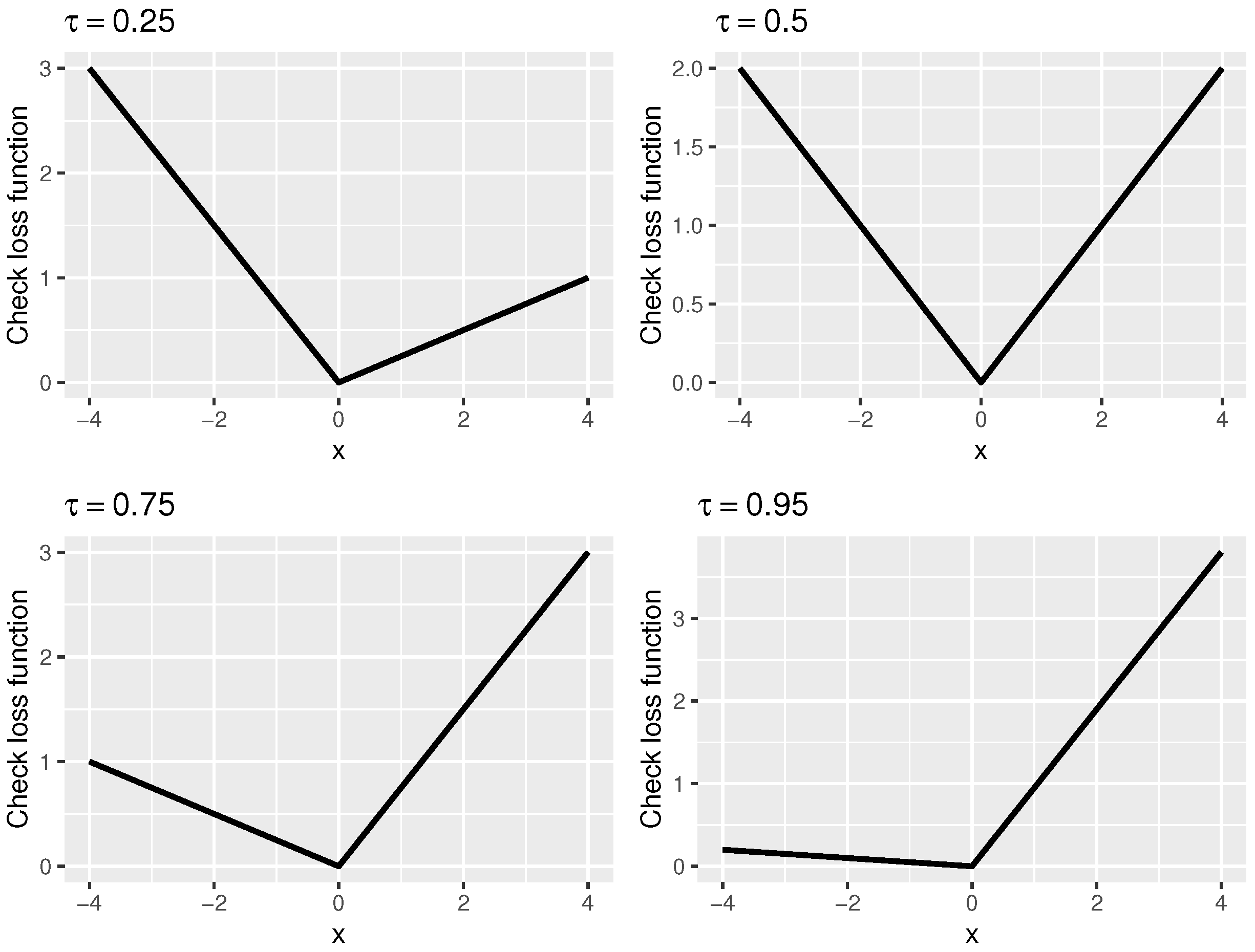
where is the piecewise linear check loss and represents the quantile level. In Figure 1, we show the loss function for different values of . When , the loss function becomes . To see why this makes sense, we note that it is well-known that given a sample , the minimizer of is the sample median (the minimizer of the least squares loss is the sample mean). For other values of , the loss function has a similar shape to absolute value function but is skewed so that it can recover other quantiles. For details, see [6]. The intercept would be omitted in the following for the simplicity of notation.
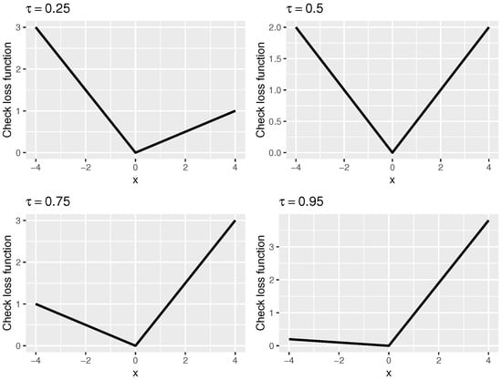
Figure 1.
The curves of the piecewise linear check loss function at .
A subgradient of the check loss function is . With an initial value , we can apply the iterative hard thresholding algorithm, which is a projected gradient descent method for the nonconvex case, to compute the estimator iteratively as
where denotes the step size. After a sufficiently large number of iterations T, we set . In the above, the projection operator enforces the constraint by retaining s elements with the largest absolute values (in magnitude) and setting the other entries of to be zero.
2.2. Distributed Estimation
In this subsection, we apply the communication-efficient surrogate likelihood (CSL) framework, proposed by [17], to solve -constraint quantile regression.
We first review the definitions and notations required in the distributed framework. In a distributed setting, N observations are randomly and evenly distributed to m machines with n observations stored on each one. Let be a set of observations independently and identically distributed with the distribution , where } is a family of statistical models parameterized by . Here, is the parameter space and is the true parameter generating the data set. In a regression problem, we have . We use to denote the n observations stored on the jth machine. In particular, stands for the data on the first machine, which is regarded as the central machine (server) that can directly communicate with all others, while other machines are worker machines that can only communicate with the central machine.
Ref. [17] presented a surrogate loss function to approximate the global loss function, from which we can derive the surrogate loss function for the quantile regression model as
where is a suitable initial estimator. For example, can be the minimizer of the empirical loss function on the first machine. is the local loss function on the first machine and is the subgradient of , that is, , . is the global loss function based on all observations, and is the subgradient of . To understand the meaning of in (2), we note that the first term is the loss based on data on machine 1. The desired global loss is . Thus, to correct for the difference between and , the second term in (2) adjusts the gradient of the loss at the current estimate , to make approximate better.
Using the surrogate loss function, the communication-efficient distributed estimator is
In practice, we apply IHT to compute the distributed estimator , noting that the subgradient of the surrogate loss function is . Note that to obtain in the distributed setting, needs to be broadcast to all local machines and the local subgradients are computed on all machines and sent to the central machine to form the global gradient .
We can repeat the above procedure for multiple stages. In stage t, we set the starting value to be the estimator obtained in the previous stage, and then form the surrogate loss function
and then obtain by minimizing the surrogate loss function above (using IHT)
which serves as the initial value for the next stage (see Algorithm 1 for pseudocode).
Remark 1.
For convenience of presentation only, we assume data are evenly distributed on all machines. However, when the total sample size N is fixed, the only important quantity is the sample size n on machine 1, which determines the accuracy of the initial estimator, as well as the surrogate function, while sample sizes for other machines play no role since other machines only contribute the gradients and all gradients are aggregated by machine 1.
To see this point more clearly, in (2), the only term that requires the participation of other machines is the term . Whatever the local sample sizes for machines , denoted by , each machine simply sends , and machine 1 can aggregate them by an weighted average to obtain exactly . Alternatively, the machines can simply send the sum of gradients on observations (instead of the mean of gradients on observations) and then machine 1 can sum up these quantities and divide it by N, to obtain exactly .
| Algorithm 1 distributed estimation for quantile regression using IHT |
|
3. Main Results
In this section, we provide the theoretical result showing the convergence rate of the distributed estimator. We will see that the distributed estimator can achieve the same convergence rate as the global estimator based on the whole data set under suitable assumptions. We note that the check loss function for quantile regression is neither strongly convex nor second-order differentiable, and constraint is nonconvex, which renders the theory in [17] not directly applicable to our current problem.
Let be the conditional density of (as defined in (1)). The following assumptions are imposed.
- (A1)
- Define and (it can be shown that actually contains the second-order partially derivatives of and is thus referred to as the population Hessian matrix). We assume that is bounded from above by a constant and is bounded from below by a constant , for all -sparse unit vectors (that is, ).
- (A2)
- Components of are sub-Gaussian random variables in the sense that for any and some positive constants .
Assumption (A1) imposes a constraint on the population Hessian matrix. To see that is the Hessian matrix (in other words, it contains the second partial derivatives of ), we note that it is easy to see the first-order partial derivatives (gradient) are given by , where denotes the conditional distribution function of y. Thus, taking the derivative with respect to gives us . This is the quantile regression counterpart of the standard assumption in least squares regression that usually requires that eigenvalues of are bounded from above and below by some positive constants. This assumption is also adapted to deal with the sparse regression case where we only need to deal with a sparse unit vector . Assumption (A2) requires the predictors to be sub-Gaussian, which is necessary for our technical analysis using empirical processes theory.
In the following, C will denote a generic positive constant whose value may vary in different places. In the statement of the theorem, and are constants bounding the eigenvalues of the population Hessian matrix as in (A1). and are the initial estimator and the final estimator output by our algorithm, respectively.
Theorem 1.
Under the assumptions (A1) and (A2), let , with large enough such that ; when the initial estimator satisfies , after stages with iterations for each stage using IHT, with a probability of at least , it holds that
where denotes .
Remark 2.
We require the initial estimator to be sufficiently accurate, with . This can be guaranteed when is computed on the first machine using its local data of size n if n is not too small, as shown in [5]. Intuitively, the initial estimator should be sufficiently accurate for the surrogate loss to be a good approximation of the global loss. If the initial estimator is not accurate enough (for example in our simulation later, this is the case when the local sample size n is small), the method might have bad performance.
Remark 3.
The iterative bound for the estimation error is shown in (A11) in the proof, which indicates that the distributed estimator can be linearly convergent to the true parameter . Compared to the iterative bound for the non-distributed global estimator provided by [5], which is , we can conclude that the distributed estimator can achieve the same convergence rate as the estimator with all data stored on a single machine, when the term is the dominating term. Here, is the statistical precision since it is the error bound when using the entire sample with size N. In other words, if all data with sample size N are stored on a single machine, which performs IHT to obtain an estimator , then we have , according to the result in [5]. Thus, in this paper, we call this term the statistical precision, which is the benchmark error for the global estimator. In particular, this holds when , or equivalently, . In other words, when the number of machines is not too large, the distributed estimation has the same convergence rate as the global estimator.
4. Simulations
In this section, we numerically illustrate the convergence of the distributed estimator to verify the theoretical conclusions we obtain in Section 3, comparing it to the local estimator (only using the data stored on the first machine) and the global estimator (assuming all data are stored on a single machine). We then turn to demonstrating the robustness to different parameter setups and the accuracy of nonzero parameter identification.
4.1. Convergence Illustration
We first generate N i.i.d observations by , where is from the multivariate normal distribution with mean and the covariance matrix . The noise is generated from the normal distribution with mean 0 and variance . We set , with the dimension , . Strictly speaking, as a tuning parameter, we could use cross-validation to fix the proper value of s. Here, we solely fix s to discuss the convergence of the estimators.
We will report the estimation error (EE) of the estimators using 100 repetitions in each setting, and the prediction error (PE) based on additional independently generated 5000 observations.
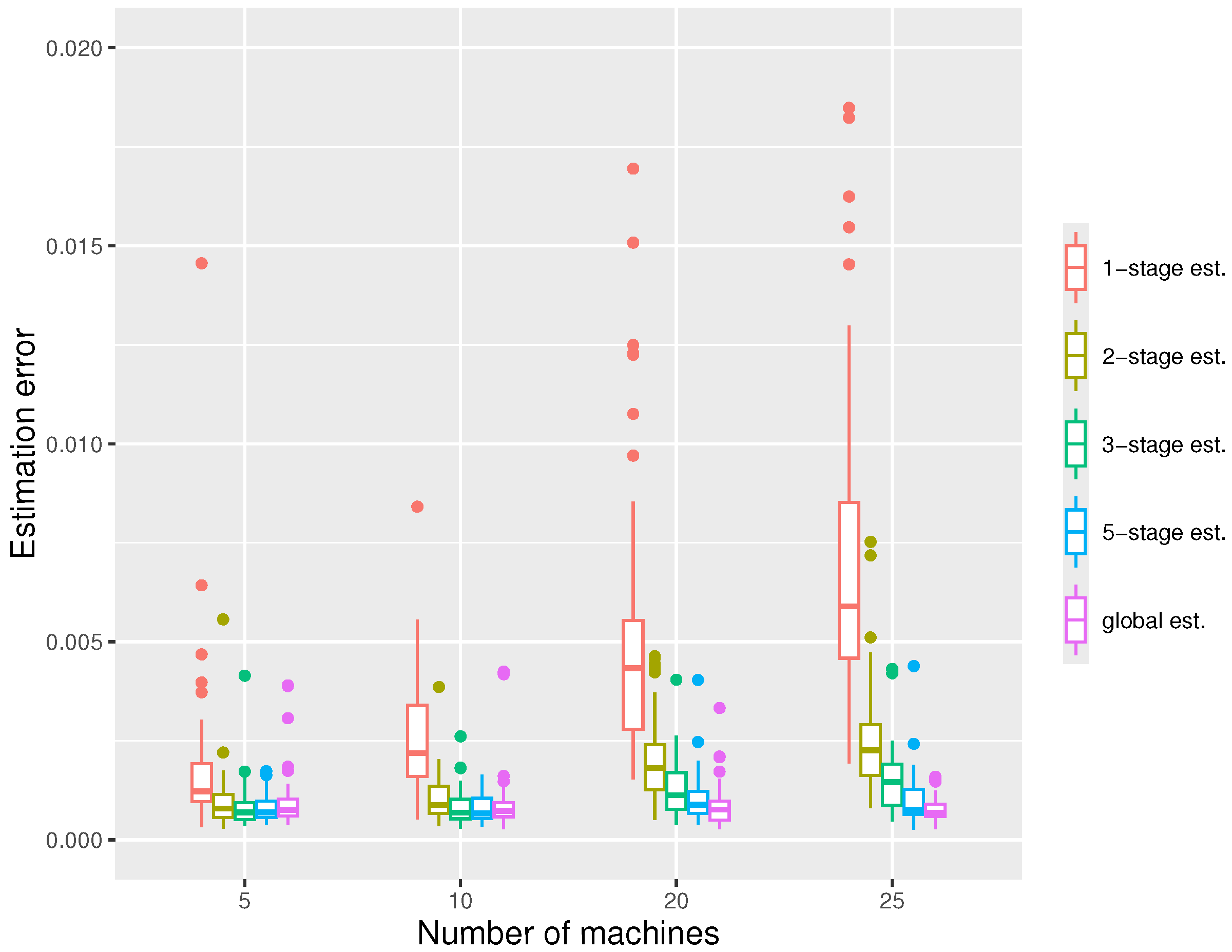
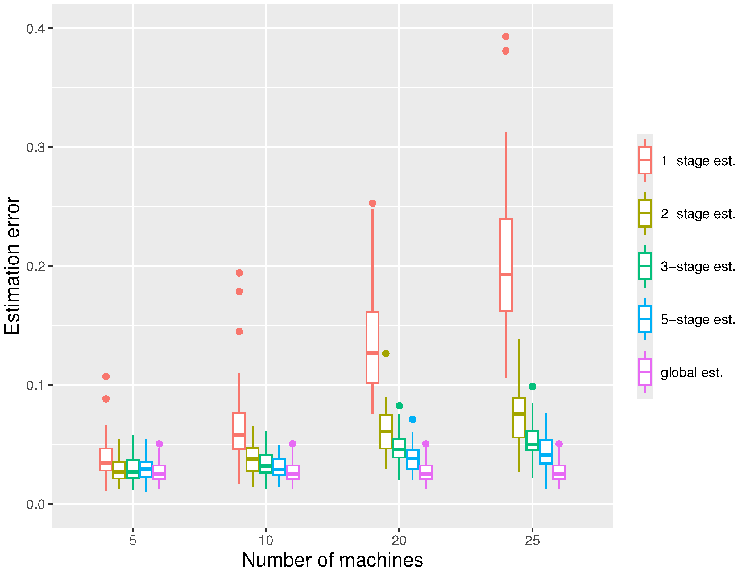
For the first simulation, we fix the whole sample size and vary the number of machines m, with the results shown in Figure 2. We can observe that the errors decrease with the number of stages used, and with a five-stage estimator, the errors are usually close to those of the global estimator. We see that the one-stage estimation is typically insufficient, with much larger errors. For , the estimator quickly converges with a very small number of stages, while for a larger number of machines, more stages are probably required. We also note that the estimation errors increase with the number of machines m.
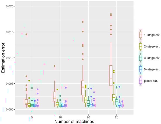
Figure 2.
The boxplots displaying the estimation errors of the distributed estimators at the -stage and the global estimator, respectively, under the settings , , at quantile level .
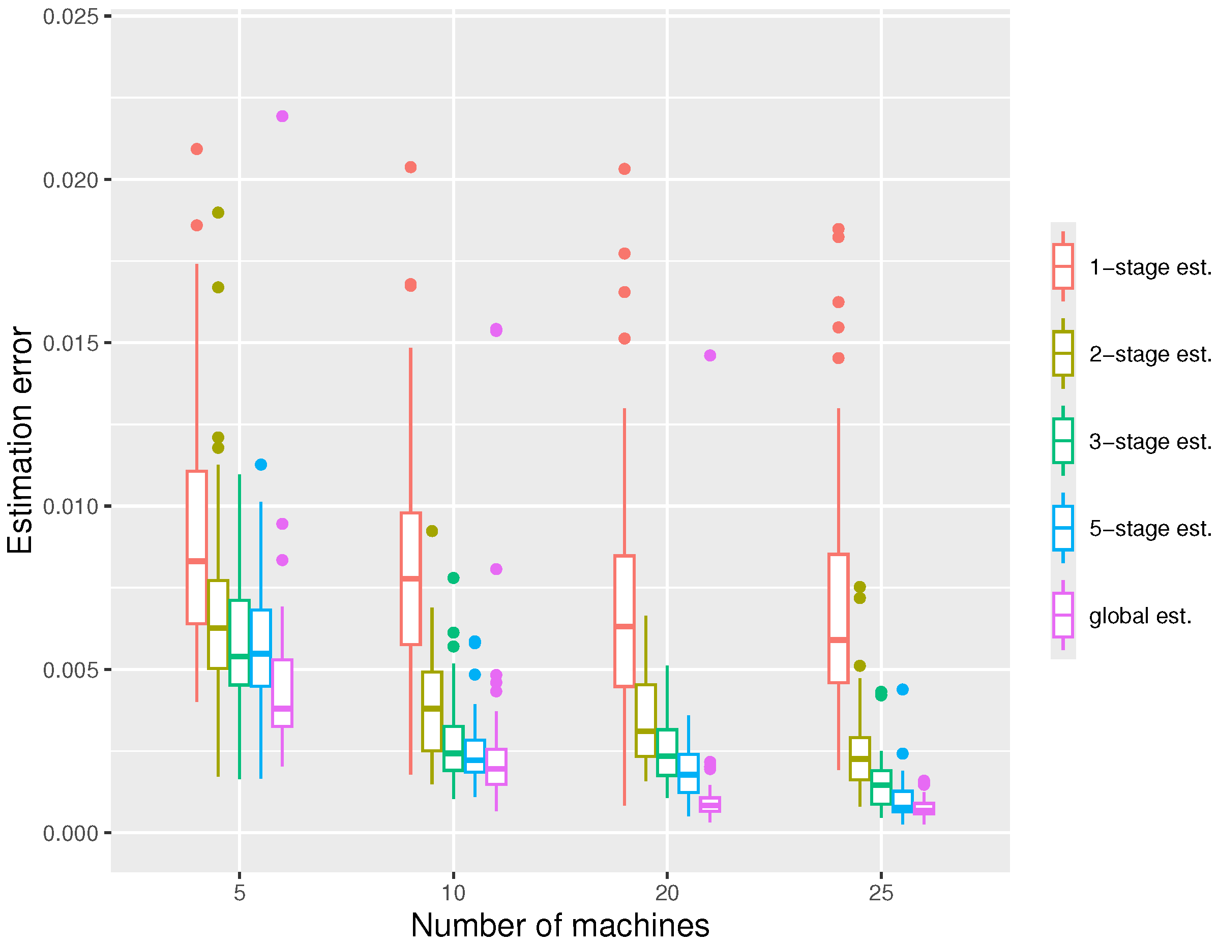
In our second simulation, we keep the local sample size fixed and increase the number of machines m. According to Figure 3, the estimation errors of all estimators decrease with m as expected, since the total sample size N is proportional to m. Again, we see one-stage estimators perform much worse than multiple-stage estimators.
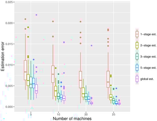
Figure 3.
The boxplot displaying the estimation errors of the distributed estimators and the global estimator respectively under the settings , at quantile level .
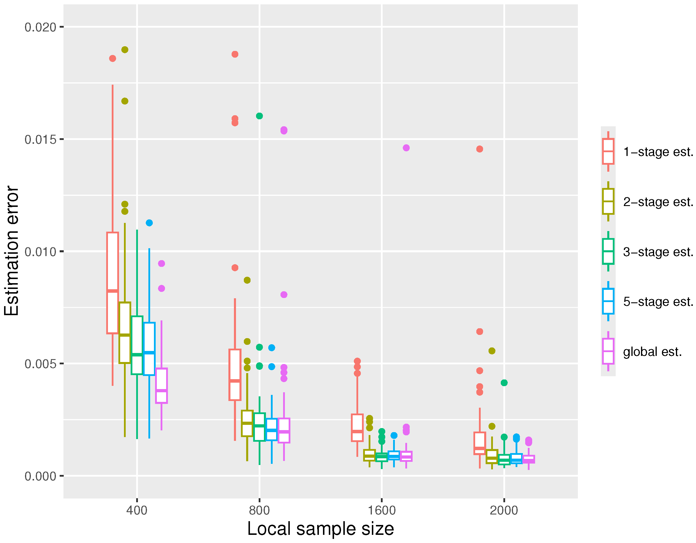
In the third simulation, we fix and increase the local sample size n. Again, we see in Figure 4 that the errors decrease with n. When the local sample size n is sufficiently large, two or three stages suffice for the distributed estimators to gain good performances comparable to the global estimators. We also note that when n is small (), there is still a significant gap between the distributed estimator and the global estimator after five stages.
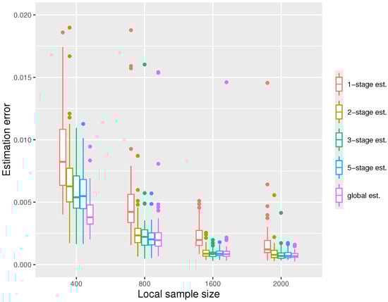
Figure 4.
The boxplot displaying the estimation errors of the distributed estimators and the global estimator, respectively, under the settings at quantile level .
We also ran experiments to verify the performance of the distributed estimator we developed in some more extreme cases. We explored the scenarios in which the number of machines m and the dimension d became large with the entire sample size . We use and a much larger . With , the local data size is , which is much smaller than . As shown in Table 1, the errors grow with the dimension d, as expected. The distributed estimator largely reduces the estimation errors of the local estimator and can decrease the errors stage by stage in high-dimensional settings. The estimation errors exhibit a surge when the number of machines is 100, showing the method would fail if m is too big.

Table 1.
The estimation and prediction errors of the local estimator , the two-stage distributed estimator , the three-stage distributed estimator , and the global estimator with , at quantile level .
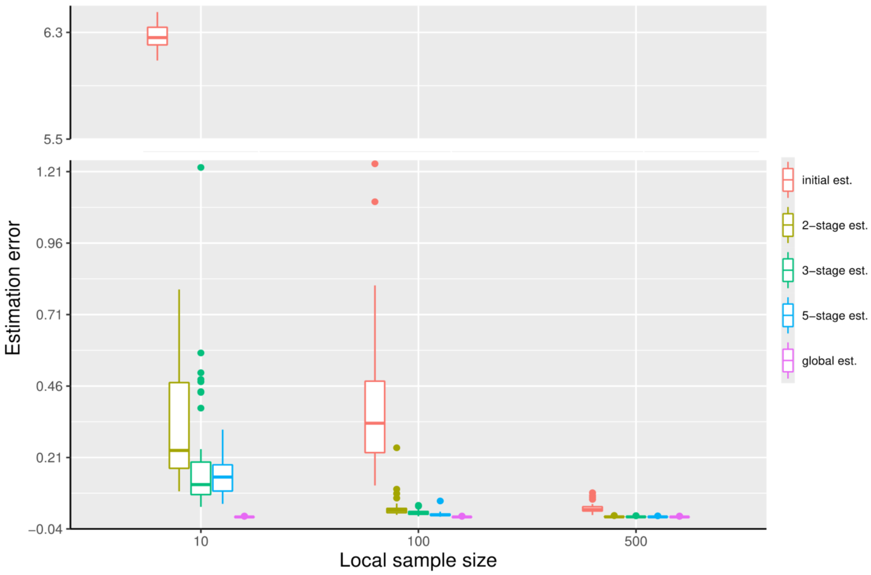
We now illustrate what happens if n is very small. We set , and , with the other settings unchanged as in the first simulation. We can observe from Figure 5 that when the first machine has significantly less data, the initial estimator would not be accurate enough. Correspondingly, the distributed estimators perform much worse, and, even after five stages, the errors are still large; increasing the number of stages further does not help.
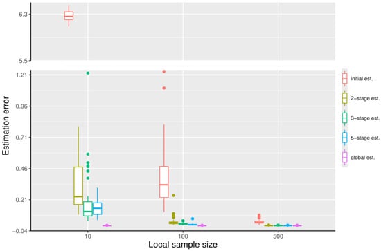
Figure 5.
The boxplots displaying the estimation errors of the initial estimator, the distributed estimators at the -stage, and the global estimator, respectively, under the settings , at quantile level .
Finally, we illustrate the convergence of the proposed distributed estimator in the case where the noise distribution is chi-squared with 5 degrees of freedom. The other settings remain unchanged as in the first simulation. The boxplots displaying the estimation errors are shown in Figure 6. We see that qualitatively, the results are similar to those of Figure 2. When m is small, the two-stage estimator is almost as good as the global estimator. When m becomes larger, more stages are required and there is a perceivable performance gap between the distributed estimator and the global estimator.
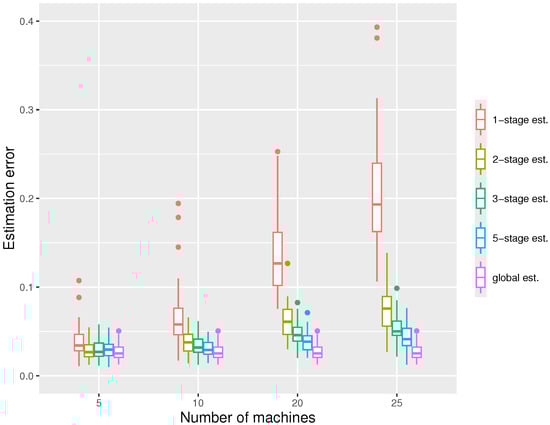
Figure 6.
The boxplots displaying the estimation errors of the distributed estimators at the -stage and the global estimator, respectively, under the settings at quantile level . The noise distribution used is chi-squared with 5 degrees of freedom.
4.2. Variable Identification Performance
In this simulation, to examine whether the magnitude of the true parameter and the sparsity affect the estimation and variable selection, we generate i.i.d observations with , where there are 50 nonzero parameters following a decreasing pattern and the dimension . Using 100 repetitions, we record the number of times each of the 100 parameters is identified as nonzero. With this, we can obtain the corresponding identification frequency. We also report the overall misclassification rate (MCR), which is the proportion of the sum of false positives and false negatives in identifying nonzero parameters.
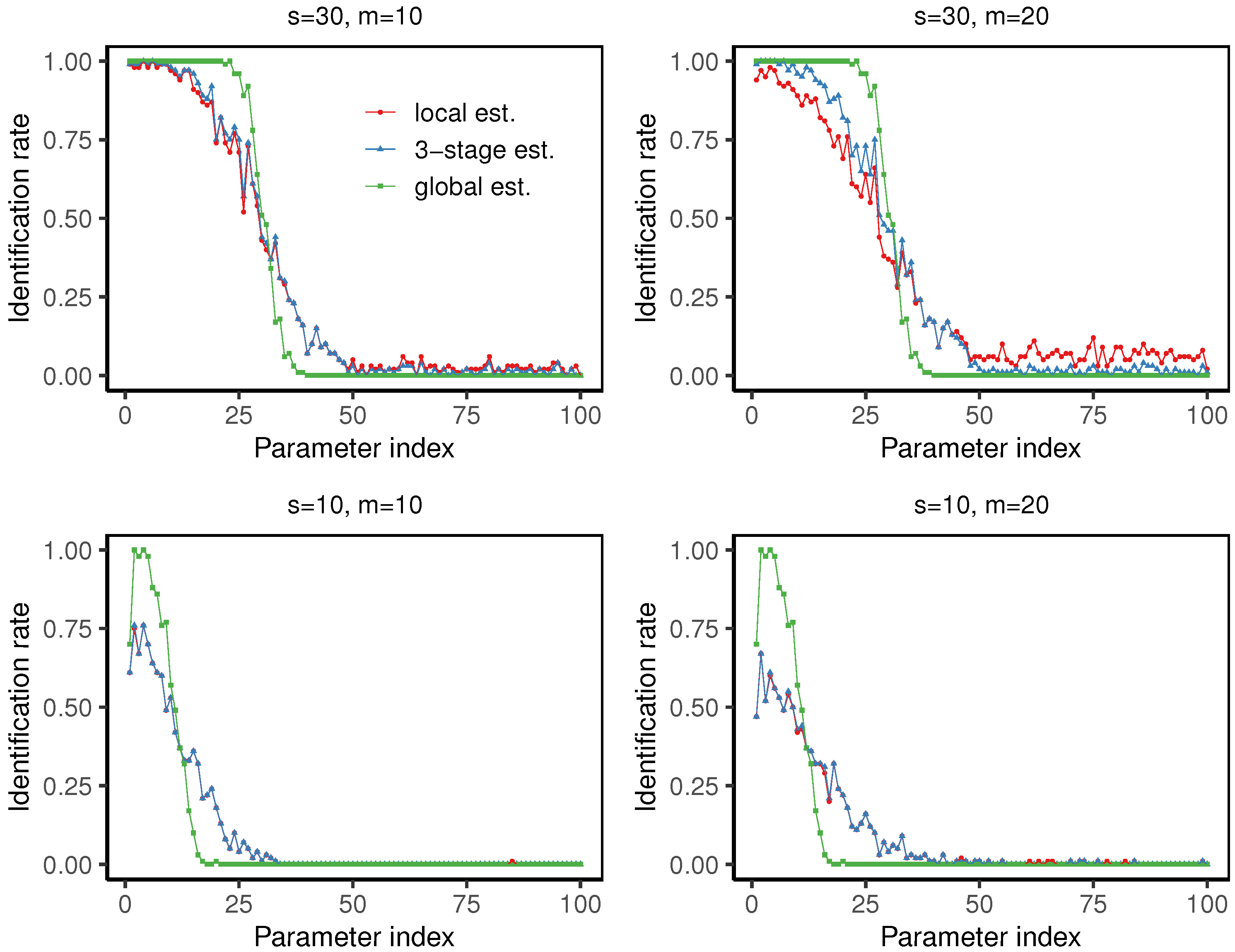
In our simulations, we set . As shown in Figure 7 and Table 2, with the special setting of , the identification rates decrease as the parameter index grows. At , the three-stage estimator slightly outperforms the local estimator, with higher identification rate for the parameters with large magnitudes and a lower misclassification rate. At , the local estimator and the three-stage estimator have almost identical performance. We can also observe that the misclassification rate of the three-stage distributed estimator increases slightly with the number of machines. In addition, we report the computational time of the four cases, each using 100 repetitions, as shown in the footnotes of Table 2. Our algorithm is implemented in R (R-4.4.2) on our desktop computer with 12th Gen Intel(R) Core(TM) i5-12400F 2.50 GHz and 16 GB RAM.
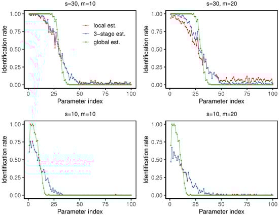
Figure 7.
The line charts displaying the identification rate of the local estimator , the three-stage distributed estimator , and the global estimator , respectively, under the settings , at quantile level . In all cases, each point corresponds to the identification rate over 100 trials for each of the 100 parameters.
Table 2.
The misclassification rate , estimation and prediction errors of the local estimator , the three-stage distributed estimator , and the global estimator with , at quantile level .
5. Conclusions
In this article, we theoretically establish the convergence rate of the distributed estimator for quantile regression with constraint. We extend the conclusions of [17] to the model with a non-smooth loss function and a nonconvex constraint. The numerical experiments show that the distributed estimators have satisfactory performance. The distributed estimator can decrease the estimation and prediction errors stage by stage. It also largely reduces the errors of the local estimator and two or three stages often suffice for the distributed framework to gain almost the same accuracy as the global estimator. The errors increase with the number of machines m when N is fixed, decrease with m with n fixed, and also decrease as n grows with m fixed.
Our work has its limitations; for example, in our simulations, we notice that only with each machine having sufficient observations can we have satisfactory performance. This is probably due to the initial estimator being important for performance, and when the local sample size is too small, the initial estimator is not good enough. This makes the proposed method sometimes unreliable in practice.
The proposed method contributes theoretically and businesswise. Existing distributed frameworks with high-dimensional statistical settings have convergence guarantees held only for smooth convex models. We bridge the gap and extend it to the non-smooth and nonconvex situation. In addition, it is effective for addressing large-scale statistical optimization problems. It divides a substantial task into smaller components that can be processed in parallel across multiple machines. This approach can be utilized by commercial companies to analyze vast amounts of browsing data and identify the most influential factors for personalized recommendations. Additionally, biological researchers may resort to this method to pinpoint the most significant genes to diagnose certain diseases.
Some extensions can be considered. For example, one can consider composite quantile regression (CQR) proposed by [18], which is regarded as a robust and efficient alternative to mean regression. One can also consider the quantile matrix regression problem, where the predictors and parameters are in the form of matrices. Also, it is well-known that standard quantile regression based on the check loss does not work for extreme quantile levels such as , for which more complicated methods such as [19] should be applied. Furthermore, we did not consider the variance estimation problem, which would be useful if we want to perform statistical inference. Furthermore, we chose one particular approach of distributed estimation for its simplicity and feasibility to demonstrate its extension to the particular non-smooth nonconvex problem that interests us; other approaches such as using DGD (distributed gradient descent) or ADMM (alternating direction method of multipliers) could also be investigated [20,21]. Finally, federated learning emphasizes the case of heterogeneous data distribution and asynchronous update [22] and is more challenging to deal with. These interesting problems are left for future work to solve.
Author Contributions
Conceptualization, H.L.; methodology, Z.Z. and H.L.; software, Z.Z.; validation, Z.Z. and H.L.; investigation, Z.Z.; resources, H.L.; data curation, Z.Z.; writing—original draft preparation, Z.Z.; writing—review and editing, H.L. and Z.Z.; visualization, Z.Z.; supervision, H.L.; project administration, H.L.; funding acquisition, H.L. All authors have read and agreed to the published version of the manuscript.
Funding
This research received no external funding.
Institutional Review Board Statement
Not applicable.
Informed Consent Statement
Not applicable.
Data Availability Statement
No new data were created or analyzed in this study.
Conflicts of Interest
The authors declare no conflicts of interest.
Appendix A. Proof of Theorem 1
Proof of Theorem 1.
Let denote the derivative of the surrogate loss function . We first focus on the first stage . Define , where and are the support (set of indices of nonzero entries) of and the true parameter , respectively. We have
where the last inequality applies Lemma 1 in [4].
By adding and subtracting terms, we obtain
Let and define
where , , and . We will show by induction that with a probability at least for all q.
Trivially, by definition. Assume . Through Lemma 1 in [5], we know that for any , with a probability at least
By sub-Gaussianity, we can obtain . When the constant C in is set sufficiently large, is very small.
By Taylor’s expansion,
where and denotes the sub-matrix with rows in . Let . Then, we obtain
where the last step is based on assumption (A1).
Finally, we have
Using Lemma 1 in [5], with probability at least ,
By sub-Gaussianity,
By our choice of which makes , we can reformulate (A10) as
where we used the Cauchy–Schwarz inequality in the second inequality. This finishes the induction step.
Using the iterative definition of , we have
Hence, after at least iterations, we have . We also note that
For other stages, we similarly have
Thus, with iterations, we have the desired bound. □
References
- James, G.; Witten, D.; Hastie, T.; Tibshirani, R. An Introduction to Statistical Learning: With Applications in R; Springer: New York, NY, USA, 2013. [Google Scholar]
- Tibshirani, R. The lasso method for variable selection in the Cox model. Stat. Med. 1997, 16, 385–395. [Google Scholar] [CrossRef]
- Shen, X.; Pan, W.; Zhu, Y. Likelihood-based selection and sharp parameter estimation. J. Am. Stat. Assoc. 2012, 107, 223–232. [Google Scholar] [CrossRef] [PubMed]
- Jain, P.; Tewari, A.; Kar, P. On iterative hard thresholding methods for high-dimensional M-estimation. Adv. Neural Inf. Process. Syst. 2014, 27. [Google Scholar]
- Wang, Y.; Lu, W.; Lian, H. Best subset selection for high-dimensional non-smooth models using iterative hard thresholding. Inf. Sci. 2023, 625, 36–48. [Google Scholar] [CrossRef]
- Koenker, R.; Bassett, G., Jr. Regression quantiles. Econom. J. Econom. Soc. 1978, 1, 33–50. [Google Scholar] [CrossRef]
- Koenker, R. Quantile Regression; Econometric Society Monographs; Cambridge University Press: Cambridge, UK, 2005; p. xv. 349p. [Google Scholar]
- Portnoy, S.; Koenker, R. The Gaussian hare and the Laplacian tortoise: Computability of squared-error versus absolute-error estimators. Stat. Sci. 1997, 12, 279–300. [Google Scholar] [CrossRef]
- Koenker, R.; Hallock, K.F. Quantile regression. J. Econ. Perspect. 2001, 15, 143–156. [Google Scholar] [CrossRef]
- Koenker, R.; Geling, O. Reappraising medfly longevity: A quantile regression survival analysis. J. Am. Stat. Assoc. 2001, 96, 458–468. [Google Scholar] [CrossRef]
- Cade, B.S.; Noon, B.R. A gentle introduction to quantile regression for ecologists. Front. Ecol. Environ. 2003, 1, 412–420. [Google Scholar] [CrossRef]
- Rosenblatt, J.D.; Nadler, B. On the optimality of averaging in distributed statistical learning. Inf. Inference 2016, 5, 379–404. [Google Scholar] [CrossRef]
- Lin, S.; Guo, X.; Zhou, D. Distributed learning with regularized least squares. J. Mach. Learn. Res. 2017, 18, 1–31. [Google Scholar]
- Lian, H.; Fan, Z. Divide-and-conquer for debiased l1-norm support vector machine in ultra-high dimensions. J. Mach. Learn. Res. 2018, 18, 1–26. [Google Scholar]
- Huang, C.; Huo, X. A distributed one-step estimator. Math. Program. 2019, 174, 41–76. [Google Scholar] [CrossRef]
- Shamir, O.; Srebro, N.; Zhang, T. Communication-efficient distributed optimization using an approximate Newton-type method. In Proceedings of the 31st International Conference on Machine Learning, Beijing, China, 21–26 June 2014; Volume 32, pp. 1000–1008. [Google Scholar]
- Jordan, M.I.; Lee, J.D.; Yang, Y. Communication-efficient distributed statistical inference. J. Am. Stat. Assoc. 2018, 114, 668–681. [Google Scholar] [CrossRef]
- Zou, H.; Yuan, M. Composite quantile regression and the oracle model selection theory. Ann. Stat. 2008, 36, 1108–1126. [Google Scholar] [CrossRef]
- Wang, H.J.; Li, D. Estimation of extreme conditional quantiles through power transformation. J. Am. Stat. Assoc. 2013, 108, 1062–1074. [Google Scholar] [CrossRef]
- Shi, W.; Ling, Q.; Wu, G.; Yin, W. Extra: An exact first-order algorithm for decentralized consensus optimization. Siam J. Optim. 2015, 25, 944–966. [Google Scholar] [CrossRef]
- Ling, Q.; Shi, W.; Wu, G.; Ribeiro, A. DLM: Decentralized linearized alternating direction method of multipliers. IEEE Trans. Signal Process. 2015, 63, 4051–4064. [Google Scholar] [CrossRef]
- Ma, B.; Feng, Y.; Chen, G.; Li, C.; Xia, Y. Federated adaptive reweighting for medical image classification. Pattern Recognit. 2023, 144, 109880. [Google Scholar] [CrossRef]
Disclaimer/Publisher’s Note: The statements, opinions and data contained in all publications are solely those of the individual author(s) and contributor(s) and not of MDPI and/or the editor(s). MDPI and/or the editor(s) disclaim responsibility for any injury to people or property resulting from any ideas, methods, instructions or products referred to in the content. |
© 2025 by the authors. Licensee MDPI, Basel, Switzerland. This article is an open access article distributed under the terms and conditions of the Creative Commons Attribution (CC BY) license (https://creativecommons.org/licenses/by/4.0/).