Abstract
This paper focuses on explaining changes over time in globally sourced annual temporal data with the specific objective of identifying features in black-box models that contribute to these temporal shifts. Leveraging local explanations, a part of explainable machine learning/XAI, can yield explanations behind a country’s growth or downfall after making economic or social decisions. We employ a Local Interpretable Model-Agnostic Explanation (LIME) to shed light on national happiness indices, economic freedom, and population metrics, spanning variable time frames. Acknowledging the presence of missing values, we employ three imputation approaches to generate robust multivariate temporal datasets apt for LIME’s input requirements. Our methodology’s efficacy is substantiated through a series of empirical evaluations involving multiple datasets. These evaluations include comparative analyses against random feature selection, correlation with real-world events as explained using LIME, and validation through Individual Conditional Expectation (ICE) plots, a state-of-the-art technique proficient in feature importance detection.
Keywords:
artificial intelligence; FLAML; imputation; Local Interpretable Model-Agnostic Explanation; machine learning; XAI MSC:
68T01
1. Introduction
LIME [1] has traditionally been used to dissect and interpret model predictions. Its adaptability has been shown in areas such as time series data analysis [2] and the interpretation of cardiographic signals [3]. It has been pivotal in formulating explanations that precisely illuminate a model’s workings [4]; however, previously, LIME has been modified to handle time-series data and explain changes in predictions. We believe that the base version of LIME [1] will work with annually collected temporal data.
Thus, this paper investigates temporal data collected from global sources [5] on an annual basis. Our primary focus lies in the effective utilization of advanced data analytics to forecast emerging trends and identify avenues for improvements at the national level. The insights gained from these analyses have far-reaching implications, including the potential to guide policy reforms that could significantly improve the well-being of citizens. Furthermore, our work offers valuable perspectives on the key factors that play a pivotal role in shaping a country’s economic direction, among other applications.
A significant innovation in this study is the extension of LIME’s scope to encompass datasets featuring multiple time-series, selecting features that can best explain a change in the target feature. Previous works have built upon LIME to work with time-series data [6], but LIME, without any modifications, can work with temporal data; we show that its selected features align with real-world cases.
In addition, LIME is deployed to scrutinize predictions generated by models fine-tuned using FLAML [7], a Python library adept at autonomously pinpointing optimal hyperparameters across a spectrum of black-box models. By delving into an assortment of such models, this research aims to showcase LIME’s proficiency in distilling these models and explaining the foundational rationale of their predictions. In addition, it offers information on how changes in features influence the predicted outcomes, improving user comprehension.
This study employs three open-access temporal datasets that capture variations in national happiness levels [5], economic freedom [8], and population dynamics [9]. We assess the validity of our approach through a series of tests that include benchmarking against randomly selected features, establishing correlations with real-world occurrences as interpreted using LIME, and cross-validating outcomes using Individual Conditional Expectation (ICE) plots [10], a leading method for determining feature significance. The focus lies on the precision of LIME in feature identification, supported by concrete case studies that authenticate its predictive claims, regardless of whether they carry positive or negative implications.
2. Related Work
Introduced in 2016, LIME aims to understand black-box models by generating interpretable and accurate predictions via the creation of a more transparent model [1]. This transparency is achieved by iteratively sampling the intricate model to approximate its behavior. Given LIME’s approach of treating the model as a black box, it exhibits model-agnostic properties. Then, from LIME’s recreation of the model, individual points can be provided for LIME to provide explanations on. This approach was expanded upon by several researchers who noted that LIME lacked any support for time-series data with thousands of entries, such as hourly weather updates or stock prices, leading the proposal of LEFTIST, the first model-agnostic approach for time series data [2], which segments the time-series data into several components of equal length. This was followed by TS-MULE [6], which approaches several problems like how to properly segment the time-series into several windows of different lengths, such as SAX segmentation, and then suggests several transformations. Finally, LIMESegment was developed a year later [11], which outperforms previous research with an approach involving frequency distributions and understanding the local neighborhood of a time-series.
Previous work has also been done in terms of applying LIME to various datasets, since LIME is highly successful and can be easily applied to textual, tabular and image data. For example, LIME has been used to categorize plants’ species after InceptionV3, XCeption, and ResNet50 models were trained [12], to show why image captioning models selected certain words to be part of an image caption [13] and to classify healthy and unhealthy hair through pictures of various scalps in order to detect diseases such as folliculitis decalvans and acne keloidalis, with a high accuracy of 96.63% from the black box model that was backed up with explainable machine learning. A further history of LIME and its’ studies can be found in Table 1.

Table 1.
A History of recent studies (2019 or later) in LIME.
Several other applications exist, such as using LIME in conjunction with other approaches like Shapley Values, to explain why users could potentially have diseases like diabetes and breast cancer [20]. LIME has also been used to provide real-world explanations for why a synthetic dataset of various machine parts would suffer breakdowns, with the explanations being provided based on the damage to the parts, as well as the temperatures that they were exposed to [21]. From the observations, it is evident that LIME can efficiently generate insightful explanations for a model, provided that the model is precise and that the data type is compatible with LIME or its variants like LIMESegment. However, for the scope of this study, LIMESegment and other approaches to univariate time-series are not valid choices, since LIMESegment works with univariate time-series, not multivariate ones. Thus, an algorithm like LIMESegment will only be able to look at the year column and the target value, instead of combining them with other features to glean more information. Therefore, a strategy that encapsulates the entirety of the data and works with any tabular dataset, not just a specific group of datasets, is essential, ensuring that the model has an optimal amount of data for processing.
3. Methodology
3.1. Problem Definition
In this study, our objectives are twofold. Firstly, given an input , we aim to predict the target label y with the highest accuracy utilizing sophisticated models. The data at hand might necessitate imputation and are bound to undergo adjustments for temporal scrutiny. The adoption of intricate models serves to demonstrate LIME’s capability to render a model more comprehensible, irrespective of its inherent complexity. Formally, LIME can be mathematically represented as Equation (1). Here, L denotes the loss, capturing the discrepancy between LIME’s approximated model—in this case, a linear model g—and the actual model f. delineates the extent of the vicinity around , the point that was passed into LIME, where the vicinity is where points will be sampled, while signifies the model’s complexity. Both L and should be minimized.
Secondly, our aim is to showcase the precision and capabilities of LIME when applied to the adapted data. This is achieved by comparing LIME’s outcomes and predictions with real-world instances and by contrasting the Individual Conditional Expectation Plots with LIME’s adaptation of the Submodular Pick [10]. The latter addresses an NP-Hard challenge, where the objective is to generate explanations for points, ensuring maximal distinctiveness. The underlying mathematics for the submodular pick algorithm can be shown through Equations (2) and (3).
Equation (2) offers a definition of coverage by examining V, a collection of instances, alongside W, representing the local significance of each instance. symbolizes the global prominence of a specific element within the explanation domain. The formulation of is contingent upon the data type and can be refined for enhanced efficiency. Equation (3) focuses on the pick problem, striving to amplify the cumulative coverage achieved by selecting multiple local instances. This is realized by leveraging the values computed from Equation (2).
3.2. Data Collection
Three datasets were collected for the purpose of this experiment, where the first originates from the World Happiness Report [5], the second was collected from Kaggle [8], which was initially sourced from the Fraser Institute, and the third comes from the U.S.A.’s Census Bureau [9]. Each dataset is predominantly numerical, aside from the names of countries. Additionally, the values in the first two datasets range from 0 to 10. These datasets were selected as they did not use artificial data; thus, extreme fluctuations in happiness or economic freedom between two years can be further analyzed in case studies.
- Dataset 1: The World Happiness Report dataset [5] compiles yearly data from 2015 to 2022 by gathering polls from thousands of citizens to understand how they feel about their country, and these results are then used to predict a happiness score. Over the years, the data collection methods, naming conventions, and columns have evolved. The final dataset retained columns such as Country Name, Year, Life Ladder, GDP per Capita, Social Support, Healthy Life Expectancy, Freedom to Make Life Choices, Generosity, Perception of Corruption, and Dystopia + Residual. Country names that changed from 2015 to 2022, like Swaziland to Eswatini, were manually updated. This dataset was chosen to investigate if any particular features would greatly affect a country’s happiness score.
- Dataset 2: The second dataset was originally published by the Fraser Institute and later reformatted on Kaggle [8], which focuses on the economic freedom of various countries. It is organized into five main categories, each containing multiple sub-categories, totaling 25 factors. Each country’s economic freedom score lies between 0 and 10. Such categories include military interference, inflation, business regulations, etc. The dataset’s linear relationships allow for a relatively easy calculation of a country’s economic freedom, yet they also serve as a useful tool for case studies and evaluating the effectiveness of LIME with FLAML-trained models.
- Dataset 3: The third dataset is a comprehensive set of data published by the U.S.A. [9], which tracks countries’ population year by year and provides a detailed background of its sex ratio, fertility rate, life expectancy, mortality rate, and crude death rate, among other factors. This dataset provides hypothetical estimates of the population up to 2100, but, for the sake of realism in this report, the dataset has been truncated at 2023. This dataset aims to evaluate how real-world non-calculated Y-column data performs in temporal analyses and when using the LIME approach.
3.3. Preprocessing
- Addressing Missing Data: Managing data with missing values is a pivotal issue in both data analytics and model building. This concern is especially pronounced in our investigation involving the second dataset, where nearly of the entries had at least one column with missing data. To tackle this challenge, we utilized three distinct imputation methods, ultimately selecting the best-performing approach for data imputation. This process is illustrated with Algorithm 1.
- Linear Regression Imputation: To predict missing values, we treat the feature with missing data as the dependent variable and use the other features which are complete (or mostly complete) as the independent variables. Formally, if a value is missing, its imputed counterpart can be calculated using the following equation:Here, represent the estimated coefficients obtained from the linear regression model trained on the observed data. The imputed value then takes the place of the missing value. Before using the model for imputation, we adopt Ordinary Least Squares (OLS), which minimizes the sum of the squared differences between the observed and predicted values, to estimate . This approach intuitively leverages relationships between variables to estimate absent data, ensuring that the inherent correlations in the dataset are considered.
- KNN imputation: We estimate a missing value by considering its ’k’ most similar data points (neighbors) that have no missing values for that specific feature. The task is further divided into two steps:
- (a)
- Finding neighbors: We identify the k nearest neighbors based on the Euclidean distance metric:
- (b)
- Computing the imputed value: The imputed value is then calculated as the weighted average of these k neighbors:where are the weights corresponding to the inverse of the distance to the neighbors.
This method offers the advantage of flexibility, as it is suitable for both numerical and categorical data and does not rely on linear assumptions, allowing for it to handle non-linear relationships in datasets effectively. However, the method can be computationally intensive, especially for large datasets, due to the need to calculate distances and identify nearest neighbors. - Iterative imputation: We take a stepwise approach to model each feature with missing values as a function of other features in an iterative manner. The process begins with an initial imputation with mean values. Each feature with missing values is then treated as a dependent variable, with the remaining features acting as independent variables. The missing values are predicted iteratively, cycling through each feature, until the imputations stabilize. Mathematically, the imputed value for a missing entry at iteration t is given by , where are the estimated coefficients and is a random residual.
| Algorithm 1: Imputation Algorithm for Missing Data |
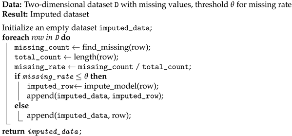 |
In this work, the linear regression imputation was selected due to its superior performance in retaining the quality of the dataset, in contrast to KNN Imputation and Iterative Imputation, which resulted in a decline in the score by 0.08–0.1 in tests. Additionally, we chose to impute rows which had 8 or fewer missing columns, which set a threshold for a row, where a row must have at least 75% of its possibly missing data available in order to have its remaining columns imputed. We selected 75%, as in a similar study [22], imputation tests that used a separate model remained relatively stable at thresholds of 80%, but collapsed more at 70%. Thus, 75% was selected as the threshold.
Dataset 2 had 36 columns, and 33 of them could have missing values. This allows for a good balance between the amount of data imputed and the quality of data, since around 1000 rows were saved using this technique.
- Reformatting data for analysis: Our primary goal here is to discern which features most significantly influenced the shift in a country’s performance, rather than focusing on specific yearly values. Given the distinct characteristics of each dataset, tailored strategies were adopted to reformat the original data into temporal multivariate time-series datasets. For the first and second datasets, apart from the country names, each row’s values were deducted by the preceding row’s values, provided that both rows pertained to the same country. This process enabled the capture of year-to-year changes. However, the third dataset, because of its unique structure, required a different approach. The only column where differences were computed was the population. For other columns, values from the preceding row were directly used to emphasize relative proportions rather than absolute variations between columns. It is worth noting that these strategies have the potential to be extended to various applications that possess a similar data format. Random samples are shown in the Appendix to demonstrate the unique nature of different datasets.
3.4. Building Models with FLAML
Once this was performed, the countries’ names were encoded into numerical values, for the purpose of being able to use them with LIME later on. The data were then split into 80–20 splits and trained using the FLAML Python package FLAML [7]. FLAML is built for machine learning, particularly for cost-effective hyperparameter optimization for ensemble classification and regression methods. The statistic that should be optimized, such as the model’s RMSE or value, can be manually selected, as well as the amount of time to be given to the algorithm, and the algorithm will provide regular updates on its progress. As seen in Figure 1, the models built by FLAML, whether they are built with Light GBM or ExtraTrees, provide a near-optimal fit for the data, with the line of best fit being a nearly perfect diagonal line. FLAML also leans towards specific models based on the data and will iterate more on more suitable models; for example, for Dataset 2, FLAML tends to always select Light GBM as the model used, and, for Dataset 3, FLAML tends to avoid models like Random Forest. Within this work, we use FLAML in order to train accurate and complicated models in order to show the utility of LIME and to ensure that LIME is truly being tested, not the abilities of FLAML.
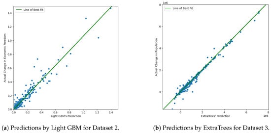
Figure 1.
Predictions by different models for Dataset 2 and Dataset 3.
3.5. Interpreting with LIME
While complex models, such as deep neural networks or ensemble methods generated using FLAML, offer high accuracy, they often lack transparency, making it challenging to understand their decision-making process. LIME addresses this by locally approximating the black-box model’s predictions. For a given prediction, LIME generates a set of perturbed data samples, obtains predictions for these samples from the black-box model, and then fits a simpler, interpretable model to these samples, typically a linear regression model. LIME figures out what the most effective columns are through these perturbations [23]. For example, if changing the value of the country’s area greatly affects the prediction for the country’s population, then this might be an important feature. Consequently, if changing a feature affects the result by a minor amount or not at all, then the feature is not important.
For this purpose, we set to and 9000 for three datasets, respectively, where the kernel width determines the width of the neighborhood of points around the data point that is allowed to influence the local model and, consequently, the explanation. The models built using LIME serve as a proxy to the black-box model, but are transparent in their decision-making. In order to properly test the quality of LIME, we ran comprehensive tests, where LIME made predictions for the entire test set in the case of the first two datasets and for the first 250 rows in the case of the third test set, while being restricted to a set number of columns, with that number being 3 for the first dataset and 10 for the other two datasets. The remainder of the rows’ values were set to 0. The R2 values were collected and were compared to cases where the same number of columns were randomly selected alongside the original model’s R2 values. Therefore, we can show that LIME’s selection of columns is significantly better than randomly selecting columns, as the brilliance of LIME lies in its ability to provide insight into the black-box model’s predictions for individual data points rather than a global approximation.
To further justify the results we received from LIME, we compare its results with those derived from Individual Conditional Expectation (ICE) plots [24], which are a tool used for visualizing the model predictions for individual instances as a function of specific input features. ICE plots are an extension of Partial Dependence Plots (PDPs) [25], which show the average prediction of a machine learning model as a function of one or two input features, holding other features constant. As ICE plots offer a nuanced view of the relationship between specific features and the predicted outcome, features with ICE lines that show significant slopes suggest that a small change in the feature value can lead to a substantial change in the prediction. A steep slope often signifies feature importance; thus, as LIME assigns importance scores to features, by comparing the top columns returned by LIME with the slopes and variations observed in ICE plots and checking if frequently selected columns have steep slopes, we can have improved confidence in whether LIME is correctly identifying important features.
4. Results and Discussions
4.1. Experiment Setting
For each run of the FLAML algorithm, a time span of s is allocated with the aim to optimize the value in our study. The hyperparameters that are selected vary with each run, as well. The value, commonly known as the coefficient of determination, quantifies the proportion of the variance in the dependent variable that can be predicted from the independent variables. Essentially, it gauges the extent to which the independent variables in a model elucidate the variability in the dependent variable. The formula for is given by the following:
In the above equation,
- denotes the observed value;
- symbolizes the value predicted by the model;
- represents the mean of the observed values.
The numerator encapsulates the squared discrepancies between the actual observations and the predictions made using the model, reflecting the variance that the model fails to explain. Meanwhile, the denominator computes the total variance present in the data. The possible range for is between 0 and 1:
- An value of 0 suggests that the model fails to explain any variability in the dependent variable around its average.
- An value of 1 indicates that the model accounts for all of the variability.
For Dataset 1, the models considered include Light GBM, Random Forest, XGBoost, ExtraTrees, and a depth-limited XGBoost. In the case of Dataset 2, only Light GBM is utilized, while for Dataset 3, all models except Random Forest are employed. These are all variants that support regression. Model selection is refined based on frequency: models that are either consistently favored or rarely chosen are omitted, allowing for the algorithm to focus on the more influential models. Initially, long short-term memory networks (LSTMs) are explored, but are later excluded due to their unsatisfactory preliminary results, even when using simpler LSTM configurations. A potential rationale for this exclusion is that all three datasets have a relatively small size, less than 100,000 rows, which hinders the LSTM’s ability to construct a sturdy model. Given the small size and complex nature of an LSTM, this leads to overfitting, while FLAML excels with tabular data and has strong regularization (L1/L2) to prevent this. The algorithm was run five times for each dataset, with the results being provided in Table 2. The mean values are included to give the viewer an overall impression of the initial results.
Table 2.
A table showing the values for each of the datasets with FLAML.
4.2. LIME’s Results
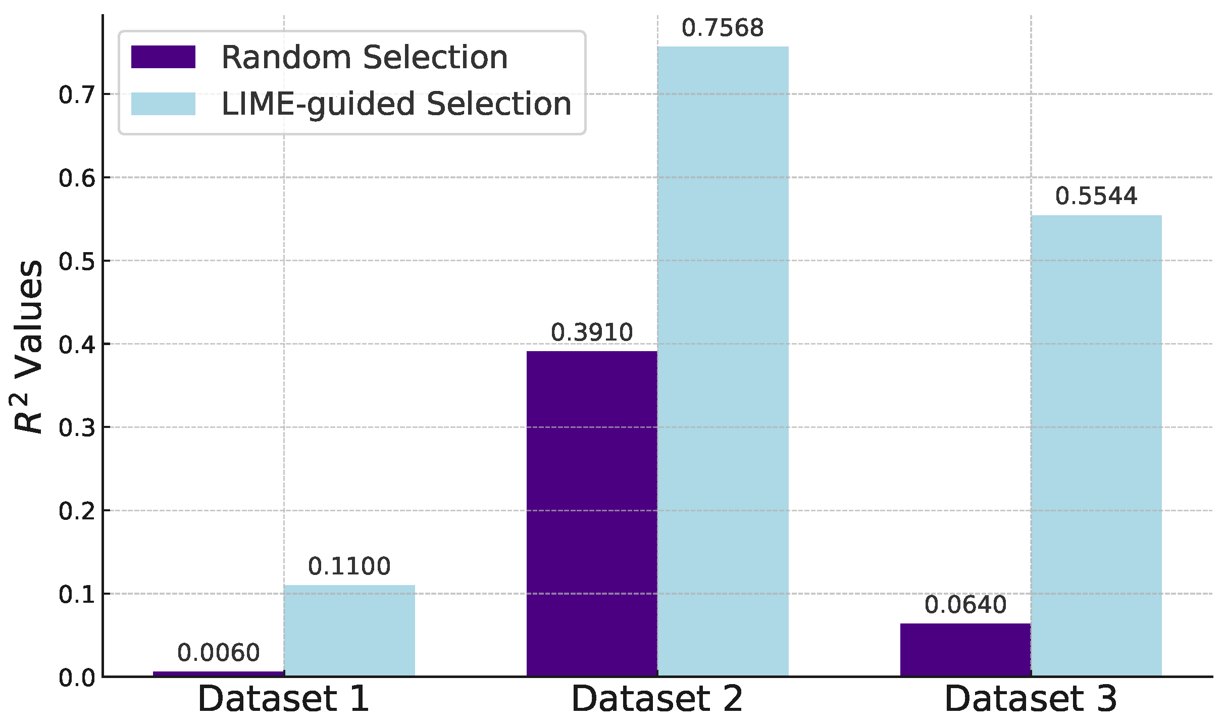
To assess the effectiveness of LIME in feature selection, we carried out multiple experiments, contrasting random column selection with LIME-guided column selection. For each of the three datasets, these experiments were conducted five times to mitigate the impact of randomness, with the average results presented in Figure 2. The closer that LIME’s scores are to the officially tested values, the better; this implies that the right features were selected. However, a perfect match is not possible, as we limit the number of columns selected; if there was no limit, LIME would simply select all of the columns as being important. Furthermore, a limit does exist; for instance, for Dataset 2, it is highly unlikely that an explanation using fewer features than the original model could surpass an score of 0.885, simply because we use the original model to gauge the quality of our explanations, and selecting fewer features would not lead to a better result.
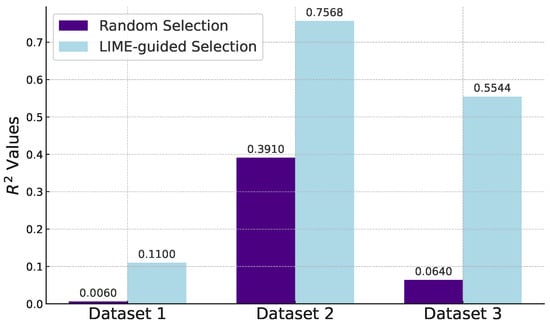
Figure 2.
A bar graph comparing the values of selecting random columns VS selecting columns with LIME.
Remarkably, across all three sets of experiments, LIME-guided feature selection consistently outperformed random selection in terms of values. This was true even for Dataset 1, which is the most difficult to understand. Moreover, there was an absolute increase in the values in every instance. This was particularly noteworthy for the third dataset, where the values surged by an average of 0.4904 when employing LIME for feature selection.
This can be further verified with an one-sided Paired T-Test, which compares the results without the use of LIME to the results with LIME. This test showed significance for the first dataset at = 0.02, while the latter two results showed significance at = 0.005, therefore, the approach that was taken by LIME was clearly statistically significant and beneficial compared to random predictions. Most notably, the P-value for Dataset 2 was 0.00005922. Dataset 1 was difficult to interpret and make predictions for, but we’ve shown that some data and insights could be discovered, hence why the R2 were significant at = 0.02, while Datasets 2 and 3 could be fully interpreted by LIME and returned excellent results for the R2 values. LIME was equally beneficial for individual predictions, as will be demonstrated through the use of real-world scenarios and ICE Plots.
4.3. Case Studies
To illustrate LIME’s efficacy, we opted for a case study approach using two extreme cases from Dataset 2. This approach not only validates the quality of LIME, but also lends real-world context to its utility. The key idea is to match significant changes in a country’s economic freedom with major historical or socio-political events and see if LIME’s explanations align with these changes.
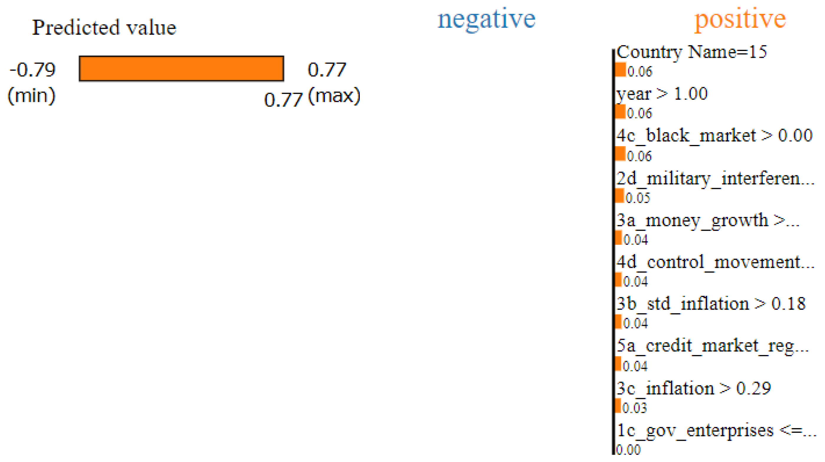
For instance, in Figure 3, Syria experienced a substantial decline in its economic freedom during 2011 and 2012, largely due to the onset of the Syrian civil war, a part of the broader Arab Spring movements [26]. In 2011, Syria’s actual economic freedom score plummeted by 0.91 points. When subjected to LIME analysis, the algorithm estimated a significant drop and associated this decline primarily with three factors: inflation, credit market regulation, and regulatory trade barriers. Their respective scores in the dataset decreased by 6.39, 1.4, and 0.56 points between 2011 and 2012, which align with the observations found in Figure 3. It is worth noting that Syria faced an inflation rate of 36.7% in 2012 [27] and also experienced severe disruptions in its business environment, leading to a mass exodus of foreign investors and tourists. These real-world factors align well with LIME’s explanation, further validating its effectiveness.
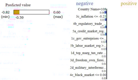
Figure 3.
A prediction made by LIME, showing the columns that most contributed to Syria’s drop in Economic Freedom between 2011 and 2012.
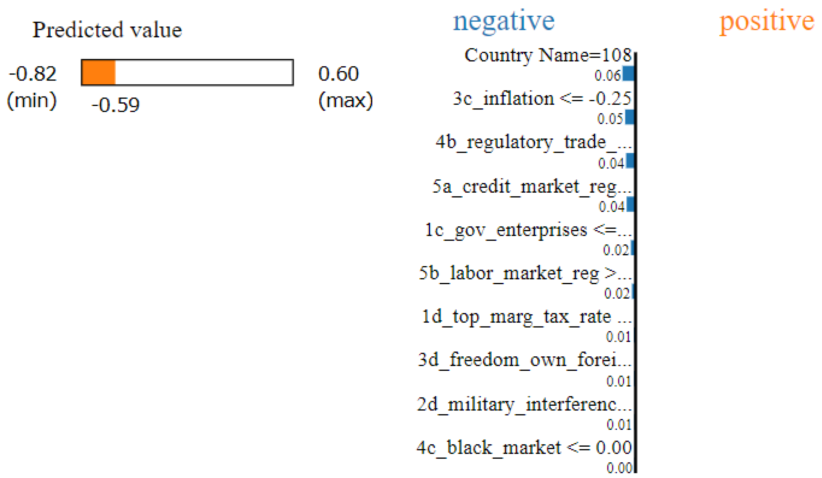
Inversely, in Figure 4, Brazil had one of the largest improvements in the dataset, with a strong comeback that took place between 1995 to 2000 and raised the country’s economic freedom by 1.32 points. This was mainly, in part, due to previous concerns that the country had in 1990–1995 being resolved. For example, Brazil suffered from massive inflation, first in early 1990 and then in 1994, with yearly rates of 2947.73% and 2075.89%, respectively; however, after the Plano Real, a stabilization program was introduced to curb this, and the largest yearly inflation from 1996–2000 was merely 15.76%, in 1996 [28]. A black market also existed due to the ineffectiveness of actual money and the need for affordable food and water. Finally, money growth also greatly increased, which is calculated through the average annual growth of a country’s money supply over the last five years minus average annual growth of real GDP in the last ten years. Annual money growth was massive in 1994 and over 6000% in 1994 [29] but would never reach such heights again and remained below 30% during the five-year period, largely in part because of the disastrous inflation being resolved.
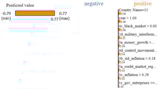
Figure 4.
A prediction made by LIME showing the columns that most contributed to the rise in Brazil’s economic freedom from 1995 to 2000.
4.4. Comparison with State-of-the-Art Methods
In order to further justify the effectiveness of LIME, we used Individual Conditional Explanation plots, acting as an extension of Partial Dependence Plots, to allow for a further analysis of LIME by analyzing the slopes of each feature. A feature with a steeper slope than other features in the ICE plot will often indicate feature importance. Thus, by comparing the columns provided by LIME with the ICE plots, we can assess the quality of LIME’s predictions and show that the ICE plots verify our results.
In our study, ICE was employed to scrutinize changes at the level of individual instances. To support this, as an example, 20 rows were chosen using LIME’s Submodular Pick function for Dataset 3, which assembles a series of local, minimally redundant explanations. The selection of 20 rows aimed to offer comprehensive coverage, align coherently with ICE plots that also focus on individual rows, and yield conclusive insights. We generated Table 3, detailing the frequency with which specific columns appeared among the top 5 chosen for these explanations. Limiting the selection to five columns rather than ten helps to concentrate attention on the most influential features. Our hypothesis posits that the features selected by LIME—due to its focus on perturbing features to identify those with the most significant impact—will corroborate their importance when examined through ICE plots, thus making them ideal candidates for generating explanations.
Table 3.
A frequency table of how LIME selects features in Dataset 3 (for 20 predictions).
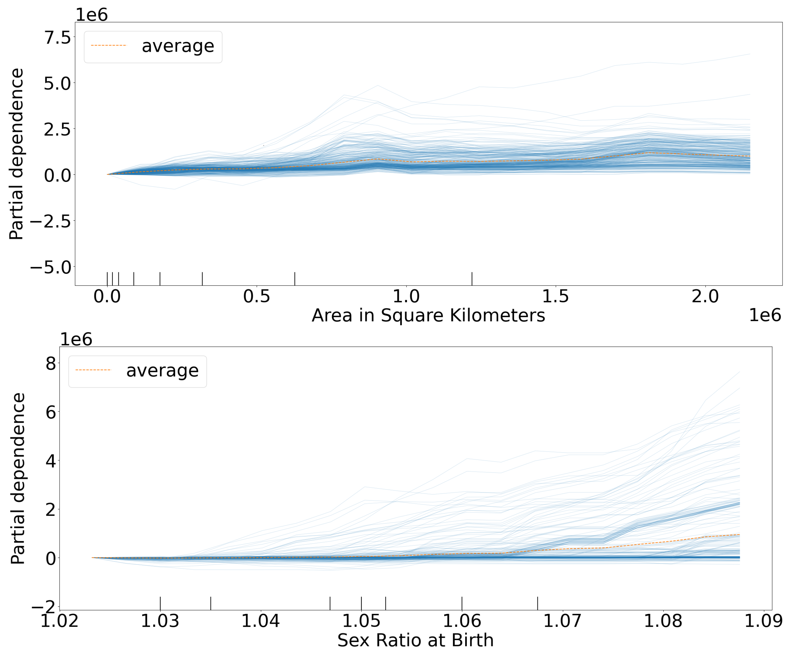
From Table 3, it is obvious that even with the algorithm trying to make the explanations as varied as possible, the feature Area in Square Kilometers was selected every single time, while Sex Ratio at Birth, Infant Mortality Rate for Females, and Under Age 5 Mortality for Females were also commonly selected.
It is clear that these selected columns are backed up by the ICE Plots in Figure 5, which all have large variances and can affect the change in a country’s population by several hundred thousand. We also noted that the features Area in Square Kilometers and Sex Ratio at Birth have the steepest slopes.
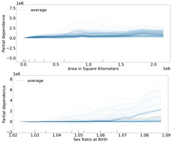
Figure 5.
ICE Plots showing how greatly the columns that are most selected by LIME affect the change in population, for Dataset 3.
It makes sense that Area in Square Kilometers would deeply impact a country’s population predictions, as it also offers a crude way to identify the country. The next several features have clear and strong correlations to a country’s population. If infants or children die, particularly female children, then that shows clear signs of a country’s instability and lack of healthcare; thus, signs point towards a lower population. Note that the infant mortality rate for males is much less important than that of females. In conclusion, LIME and ICEs both agree that these columns were the most important to Dataset 3’s predictions.
5. Conclusions
In summary, this research presents a rigorous exploration into the use of LIME for multivariate temporal analysis on global annual datasets. Our approach successfully identifies key factors contributing to temporal shifts, offering explanations that are critical for both academic inquiry and practical applications. Through the integration of LIME with other advanced methods such as ICE plots, we have not only validated the efficacy of our approach, but have also opened new avenues for explainable AI in temporal analysis.
The implementation of multiple imputation techniques to handle missing data in the second dataset exemplifies the adaptability and robustness of our method. Approximately 65% of the records in this dataset had missing values, and our strategy ensured reliable high-quality imputations that enriched the overall analysis.
Furthermore, our study lays the groundwork for future research in this area. The analytical frameworks presented here can be extended to tackle more complex datasets and questions, offering explanations behind the reshaping of governmental policies or economic strategies.
However, there are some shortcomings; this analysis could be expanded to include approaches such as Shapley Values or potentially feature permutation importance. LIME is already state of the art for explaining local predictions; thus, we ran into some difficulties with comparing our approach’s quality. Other variations on LIME, such as S-LIME, known as Stabilized LIME, could have been included. Finally, a real-world test could be performed with our approach, such as if utilizing the results from LIME’s temporal analysis could lead a subject towards or away from a future behavior.
Future research could focus on comparing the effectiveness of LIME against other explainability models or delve into real-world applications that could benefit from our approach.
Author Contributions
Conceptualization, S.N. and Y.L.; formal analysis, S.N.; data curation, S.N.; writing—original draft preparation, S.N.; writing—review and editing, Y.L.; supervision, Y.L.; funding acquisition, Y.L. All authors have read and agreed to the published version of the manuscript.
Funding
This research was funded by NSERC Discovery Grant.
Data Availability Statement
Data are contained within the article.
Conflicts of Interest
The authors declare no conflicts of interest.
References
- Ribeiro, M.T.; Singh, S.; Guestrin, C. “Why Should I Trust You?”: Explaining the Predictions of Any Classifier. In Proceedings of the 22nd ACM SIGKDD International Conference on Knowledge Discovery and Data Mining, San Francisco, CA, USA, 13–17 August 2016; pp. 1135–1144. [Google Scholar]
- Guillemé, M.; Masson, V.; Rozé, L.; Termier, A. Agnostic Local Explanation for Time Series Classification. In Proceedings of the 2019 IEEE 31st International Conference on Tools with Artificial Intelligence (ICTAI), Portland, OR, USA, 4–6 November 2019; pp. 432–439. [Google Scholar]
- Abdullah, T.A.; Zahid, M.S.B.M.; Tang, T.B.; Ali, W.; Nasser, M. Explainable Deep Learning Model for Cardiac Arrhythmia Classification. In Proceedings of the 2022 International Conference on Future Trends in Smart Communities (ICFTSC), Kuching, Malaysia, 1–2 December 2022; pp. 87–92. [Google Scholar]
- Sangani, R.B.; Shukla, A.; Selvamani B., R. Comparing deep sentiment models using quantified local explanations. In Proceedings of the Smart Technologies, Communication and Robotics (STCR), Sathyamangalam, India, 9–10 October 2021. [Google Scholar]
- Helliwell, J.F.; Layard, R.; Sachs, J.D.; Aknin, L.B.; De Neve, J.E.; Wang, S. (Eds.) World Happiness Report 2023, 11th ed.; Sustainable Development Solutions Network: New York, NY, USA, 2023. [Google Scholar]
- Schlegel, U.; Vo, D.L.; Keim, D.A.; Seebacher, D. TS-MULE: Local Interpretable Model-Agnostic Explanations for Time Series Forecast Models. In Machine Learning and Principles and Practice of Knowledge Discovery in Databases; Springer International Publishing: Cham, Switzerland, 2021; pp. 5–14. [Google Scholar]
- Wang, C.; Wu, Q.; Weimer, M.; Zhu, E. FLAML: A Fast and Lightweight AutoML Library. Proc. Mach. Learn. Syst. 2019, 3, 434–447. [Google Scholar] [CrossRef]
- Schneider, G.S. Economic Freedom of the World; Kaggle: Mountain View, CA, USA, 2018. [Google Scholar]
- U.S. Census Bureau. International database (IDB); United States Census Bureau: Suitland, MD, USA, 2020.
- Goldstein, A.; Kapelner, A.; Bleich, J.; Pitkin, E. Peeking Inside the Black Box: Visualizing Statistical Learning with Plots of Individual Conditional Expectation. J. Comput. Graph. Stat. 2013, 24, 44–65. [Google Scholar] [CrossRef]
- Sivill, T.; Flach, P. LIMESegment: Meaningful, Realistic Time Series Explanations. In Proceedings of the 25th International Conference on Artificial Intelligence and Statistics, Virtual, 28–30 March 2022; pp. 3418–3433. [Google Scholar]
- Nikam, M.; Ranade, A.; Patel, R.; Dalvi, P.; Karande, A. Explainable Approach for Species Identification using LIME. In Proceedings of the 2022 IEEE Bombay Section Signature Conference (IBSSC), Mumbai, India, 8–10 December 2022; pp. 1–6. [Google Scholar]
- Sahay, S.; Omare, N.; Shukla, K.K. An Approach to identify Captioning Keywords in an Image using LIME. In Proceedings of the 2021 International Conference on Computing, Communication, and Intelligent Systems (ICCCIS), Greater Noida, India, 19–20 February 2021; pp. 648–651. [Google Scholar]
- El Shawi, R.; Sherif, Y.; Al-Mallah, M.; Sakr, S. Interpretability in healthcare a comparative study of local machine learning interpretability techniques. In Proceedings of the IEEE 32nd International Symposium on Computer-Based Medical Systems (CBMS), Córdoba, Spain, 5–7 June 2019. [Google Scholar]
- Ramon, Y.; Martens, D.; Provost, F.; Evgeniou, T. A comparison of instance-level counterfactual explanation algorithms for behavioral and textual data: SEDC, LIME-C and SHAP-C. Adv. Data Anal. Classif. 2020, 14, 801–819. [Google Scholar] [CrossRef]
- Collaris, D.; van Wijk, J.J. Explainexplore: Visual exploration of machine learning explanations. In Proceedings of the IEEE Pacific Visualization Symposium (PacificVis), Tianjin, China, 3–5 June 2020. [Google Scholar]
- Shah, S.S.; Sheppard, J.W. Evaluating explanations of convolutional neural network image classifications. In Proceedings of the International Joint Conference on Neural Networks (IJCNN), Glasgow, UK, 19–24 July 2020. [Google Scholar]
- Zhou, Z.; Hooker, G.; Wang, F. S-LIME: Stabilized-LIME for Model Explanation. In Proceedings of the 27th ACM SIGKDD Conference on Knowledge Discovery & Data Mining, ACM, 2021, KDD ’21, Virtual, 14–18 August 2021. [Google Scholar]
- Dutta, P.; Muppalaneni, N.B. Explaining machine learning predictions: A case study. In Proceedings of the Trends in Electrical, Electronics, Computer Engineering Conference (TEECCON), Bengaluru, India, 26–27 May 2022. [Google Scholar]
- Rao, S.; Mehta, S.; Kulkarni, S.; Dalvi, H.; Katre, N.; Narvekar, M. A Study of LIME and SHAP Model Explainers for Autonomous Disease Predictions. In Proceedings of the 2022 IEEE Bombay Section Signature Conference (IBSSC), Mumbai, India, 8–10 December 2022; pp. 1–6. [Google Scholar]
- Torcianti, A.; Matzka, S. Explainable Artificial Intelligence for Predictive Maintenance Applications using a Local Surrogate Model. In Proceedings of the 2021 4th International Conference on Artificial Intelligence for Industries (AI4I), Laguna Hills, CA, USA, 20–22 September 2021; pp. 86–88. [Google Scholar]
- Guo, C.; Yang, W.; Liu, C.; Li, Z. Iterative missing value imputation based on feature importance. Knowl. Inf. Syst. 2024, 66, 6387–6414. [Google Scholar] [CrossRef]
- Molnar, C. Interpretable Machine Learning (2nd Edition). 2024. Available online: http://christophm.github.io/interpretable-ml-book (accessed on 9 February 2025).
- Yeh, A.; Ngo, A. Bringing a Ruler Into the Black Box: Uncovering Feature Impact from Individual Conditional Expectation Plots. In Machine Learning and Principles and Practice of Knowledge Discovery in Databases; Springer: Cham, Switzerland, 2021. [Google Scholar]
- Friedman, J.H. Multivariate Adaptive Regression Splines. Ann. Stat. 1991, 19, 1–67. [Google Scholar] [CrossRef]
- Atlantic Council. The Economic Collapse of Syria. Available online: https://www.atlanticcouncil.org/blogs/menasource/the-economic-collapse-of-syria, (accessed on 9 February 2025).
- Macrotrends. Syrian Arab Republic Inflation Rate (CPI). Available online: https://www.macrotrends.net/countries/SYR/syrian-arab-republic/inflation-rate-cpi (accessed on 9 February 2025).
- Macrotrends. Brazil Inflation Rate (CPI). Available online: https://www.macrotrends.net/countries/BRA/brazil/inflation-rate-cpi (accessed on 9 February 2025).
- CEIC Data. Brazil M2 Growth Indicator. Available online: https://www.ceicdata.com/en/indicator/brazil/m2-growth (accessed on 9 February 2025).

Disclaimer/Publisher’s Note: The statements, opinions and data contained in all publications are solely those of the individual author(s) and contributor(s) and not of MDPI and/or the editor(s). MDPI and/or the editor(s) disclaim responsibility for any injury to people or property resulting from any ideas, methods, instructions or products referred to in the content. |
© 2025 by the authors. Licensee MDPI, Basel, Switzerland. This article is an open access article distributed under the terms and conditions of the Creative Commons Attribution (CC BY) license (https://creativecommons.org/licenses/by/4.0/).