Abstract
This paper proposes a novel two-stage ensemble framework combining Long Short-Term Memory (LSTM) and Bidirectional LSTM (BiLSTM) with randomized feature selection to enhance diabetes prediction accuracy and calibration. The method first trains multiple LSTM/BiLSTM base models on dynamically sampled feature subsets to promote diversity, followed by a meta-learner that integrates predictions into a final robust output. A systematic simulation study conducted reveals that feature selection proportion critically impacts generalization: mid-range values (0.5–0.8 for LSTM; 0.6–0.8 for BiLSTM) optimize performance, while values close to 1 induce overfitting. Furthermore, real-life data evaluation on three benchmark datasets—Pima Indian Diabetes, Diabetic Retinopathy Debrecen, and Early Stage Diabetes Risk Prediction—revealed that the framework achieves state-of-the-art results, surpassing conventional (random forest, support vector machine) and recent hybrid frameworks with an accuracy of up to 100%, AUC of 99.1–100%, and superior calibration (Brier score: 0.006–0.023). Notably, the BiLSTM variant consistently outperforms unidirectional LSTM in the proposed framework, particularly in sensitivity (98.4% vs. 97.0% on retinopathy data), highlighting its strength in capturing temporal dependencies.
MSC:
62F15; 62G20; 62G08
1. Introduction
The widespread adoption of machine learning (ML) in prediction tasks has yet to fully address the growing global burden of chronic diseases such as diabetes, which is projected to affect 700 million people by 2045 [1]. Diabetes, categorized into type 1 (T1D) and type 2 (T2D), poses significant health risks to children and adults, respectively [1,2]. Early detection is critical for timely intervention, yet traditional ML methods, including logistic regression (LR), random forest (RF), and linear discriminant analysis (LDA), struggle with temporally structured medical data. For instance, fluctuating biomarkers like blood glucose and insulin levels require models capable of capturing longitudinal dependencies, a challenge for conventional techniques that often overlook temporal relationships [2,3].
Recent advances in deep learning (DL), particularly Long Short-Term Memory (LSTM) and Bidirectional LSTM (Bi-LSTM), offer promising solutions for sequence prediction tasks. Unlike traditional recurrent neural networks (RNNs), which suffer from vanishing gradients during backpropagation, LSTM architectures mitigate this issue through gated memory cells [1,4,5,6,7,8]. Bi-LSTM extends this capability by processing data in both forward and backward directions, enhancing sensitivity to temporal patterns [4]. Despite these advantages, diabetes research has predominantly relied on traditional ML models, which focus on static datasets and yield limited generalizability [9,10,11,12,13].
A paradigm shift is emerging in medical AI, with hybrid DL approaches demonstrating superior performance. For example, Sun et al. [2] employed Bi-LSTM to predict blood glucose levels, outperforming autoregressive (ARIMA) and support vector regression (SVR) models in reducing root mean square error (RMSE). Similarly, Kusuma et al. [14] combined convolutional and LSTM networks (CNN-LSTM) to achieve 99.5% accuracy in heart failure prediction using ECG signals, highlighting the potential of hybrid architectures for clinical applications. Cheng et al. [4,15] further advanced this trend with a knowledge-extended CNN (KE-CNN) for diabetes prediction, achieving 95.8% accuracy through entity recognition and feature selection.
Extreme Learning Machines (ELMs) have also gained traction, offering rapid training speeds and low mean squared error (MSE). Pangaribuan et al. [16] demonstrated ELM’s efficacy in diabetes diagnosis (MSE: 0.4036), while Elsayed et al. [17,18] achieved 98.1% accuracy in early-stage risk prediction. However, such studies often rely on small, non-representative datasets, limiting generalizability. Hybrid models like CNN-LSTM-SVM [19,20] and weather-predictive LSTM [21] further illustrate the versatility of sequential learning but face challenges in scalability and gradient management [3,22].
Apart from single-stage methods that solely utilize classification procedures, several hybrid methods have emerged that combine feature selection with classification techniques. For instance, ref. [23] integrated particle swarm optimization (PSO) for feature optimization with the Fuzzy Clustering Model (FCM). Similarly, ref. [24] employed principal component analysis (PCA) in conjunction with K-means clustering [25] for feature selection, subsequently using these selected features to inform logistic regression predictions. In a related approach, ref. [26] harnessed the strengths of variational autoencoders (VAEs) for sample data augmentation and sparse autoencoders (SAEs) for feature augmentation, feeding the results into a convolutional neural network (CNN) for prediction. Additionally, ref. [27] selected key features (KFs) before integrating them into an ensemble framework for predictions. ref. [7] adopted the Boruta feature selection algorithm, combining it with ensemble learning to predict diabetes.
While effective, these methods, with the exception of the Boruta approach by [7], primarily belong to the broad category of filter methods, which aim to identify key features prior to classification. These filter methods often rely on a greedy learning strategy that focuses on the most relevant features. While this approach can be effective in smooth feature spaces devoid of interactions between relevant and non-relevant features, it may falter in more complex scenarios, leading to difficulties in accurately identifying key features and, consequently, increasing false positives and diminishing prediction accuracy. In contrast, the Boruta feature selection algorithm, overlaid on a random forest procedure, exemplifies a wrapper technique. This method considers a more comprehensive feature space by randomly sampling features, thereby creating a sampling distribution that fosters diversity among base learners. This framework inspired the random feature technique utilized in the first stage of our proposed hybrid LSTM and BiLSTM models. To address the limitations inherent in existing feature selection methods, we combined the predictions from base models trained on random features using a stacking approach, enhancing overall prediction accuracy.
Despite these advancements, critical gaps remain. Many existing approaches, including Random Weighted LSTM (RWL) [28], have been validated on limited datasets such as the Pima Indian cohort, which constrains their clinical applicability. Additionally, issues such as vanishing gradients and computational inefficiencies impede real-time deployment in clinical settings. To overcome these challenges, we propose the Random Feature LSTM and BiLSTM (RFLSTM and RFBiLSTM) frameworks. These frameworks integrate dynamic feature selection and model stacking, optimizing feature diversity while leveraging temporal processing to enhance computational efficiency and generalizability. As a result, RFLSTM and RFBiLSTM present a robust solution for diabetes prediction and broader healthcare applications.
2. Random Feature Recurrent Neural Networks
The proposed method, termed the Random Feature Neural Network, is currently limited to using only LSTM and BiLSTM models; therefore, we focus our evaluation on these two RNN architectures. However, the proposed procedure is flexible and can be readily extended to other types of RNN models, including Gated Recurrent Units (GRUs), without loss of generality. Specifically, we defined the dataset as , where each represents a feature vector with p features and indicates the presence or absence of diabetes.
2.1. Random Feature LSTM
The LSTM ensemble is trained in two stages (Algorithm 1): random feature selection and LSTM training (Stage 1), followed by a second-stage LSTM model for stacking predictions (Stage 2).
| Algorithm 1 Random Feature LSTM |
|
2.1.1. Stage 1: Random Feature Selection and LSTM Training
In this stage, LSTM models are trained, each using a randomly selected subset of features, where is the desired proportion of the feature set to be selected. It is recommended that is sufficient.
For each model , the training procedure is as follows:
The predictions on training and test sets are stored as
2.1.2. Stage 2: Stacking LSTM Model
The second-stage LSTM model is trained using the meta-feature set:
where contains the predictions from the Stage 1 models. The final prediction is obtained by training another LSTM on :
Theorem 1
(lower misclassification error of Random Feature LSTM). Let be a data distribution over feature vectors and labels . Let denote a standard LSTM classifier trained on all p features and denote the Random Feature LSTM ensemble with base LSTMs trained on subsets of features (), followed by a stacking LSTM. Use the following assumptions:
- 1.
- Diversity: The base LSTMs’ prediction errors are not perfectly correlated due to random feature selection.
- 2.
- Optimality: The stacking LSTM can approximate the optimal combination of base predictions and original features.
Then, the misclassification error rate of is bounded above by that of :
Proof.
Let the misclassification error be defined as
and then the bias–variance decomposition under the squared loss can be obtained using
For classifier :
For , let be base model predictions:
We now proceed with the main results, where we assume that the Random Feature ensemble will reduce the variance of prediction. That is, for base models with predictions ,
Under diversity assumption (),
Now we proceed with the second stage of the algorithm, where we propose a stacked prediction. The stacking model receives enhanced input:
With information preservation (),
where due to the stacking LSTM’s capacity to reduce residual bias through meta-features.
Finally, combining the results, we have
Since and ,
□
Remark 1.
- 1.
- Strict inequality holds with non-zero diversity: RF-LSTM outperforms a single LSTM as long as the individual LSTM models exhibit sufficient diversity, which enables the ensemble to combine complementary information and reduce variance.
- 2.
- This requires regularization for to prevent overfitting on : The meta-classifier in the RF-LSTM framework must be regularized to avoid overfitting to the outputs of the LSTM models, ensuring that the ensemble generalizes well to unseen data.
Corollary 1
(higher accuracy of Random Feature LSTM). Let the accuracy of a classifier f be defined as
where is the misclassification error. Under the same conditions as Theorem 1, the accuracy of the Random Feature LSTM () satisfies the following inequality:
Proof.
From Theorem 1, the misclassification error rate of is bounded above by that of , i.e.,
Rewriting the relationship in terms of accuracy,
Substituting the inequality for misclassification error,
Simplifying,
This establishes that the Random Feature LSTM achieves accuracy at least as high as the standard LSTM, with the equality holding when the diversity or stacking optimization conditions are not met. □
Remark 2.
- 1.
- The strict inequality holds when the individual LSTM models exhibit sufficient diversity and the stacking LSTM effectively combines their predictions to reduce variance and bias.
- 2.
- Regularization of the stacking model () ensures that overfitting to does not degrade the ensemble’s generalization, preserving the accuracy advantage of RF-LSTM.
2.2. Random Feature BiLSTM
The procedure for the BiLSTM ensemble mirrors that of the LSTM ensemble, with the critical difference being that a Bidirectional LSTM is used in both stages (Algorithm 2).
| Algorithm 2 Random Feature BiLSTM |
|
2.2.1. Stage 1: Random Feature Selection and BiLSTM Training
For each model , the forward and backward passes are computed as
The predictions are stored similarly:
2.2.2. Stage 2: Stacking BiLSTM Model
The stacking model for BiLSTM is trained on the meta-feature set constructed using BiLSTM predictions, and the final output is
The results for the Random Feature LSTM ensemble (RF-LSTM) extend naturally to the Random Feature BiLSTM ensemble (RF-BiLSTM). We formally present the theorem, corollary, and their proofs below.
Theorem 2
(Misclassification error bound for RF-BiLSTM). Let denote the hypothesis class of a single BiLSTM model trained on a dataset , and let denote the hypothesis class of an RF-BiLSTM ensemble constructed by averaging predictions over M independently trained BiLSTM models, each using a random subset of input features. Under the assumption of independent errors across individual (diversity) BiLSTM models, the expected classification error of the ensemble satisfies
where is the classification error of a single BiLSTM model. Moreover,
Proof.
The bidirectional nature of BiLSTM improves the representational capacity by incorporating both forward and backward temporal dependencies, effectively doubling the input context for each time step. As a result, is a richer hypothesis class than , leading to
When random feature ensembles are applied, the variance reduction achieved by averaging predictions across M models further decreases the classification error, resulting in
Combining these inequalities gives
□
Corollary 2
(classification accuracy for RF-BiLSTM). Let , , , and represent the classification accuracies of their respective models. Then, the following inequalities hold:
Proof.
By definition, classification accuracy A is inversely related to classification error :
From the inequalities established in Theorem 2, we have
Substituting these into the accuracy relationship gives
□
Remark 3.
The results in Theorem 2 and Corollary 2 build upon Theorem 1 and Corollary 1 by highlighting the hierarchical relationship between LSTM and BiLSTM architectures in the context of random feature ensembles. Specifically, the bidirectional nature of BiLSTM amplifies the advantages of ensemble modelling, including reduced variance and increased robustness to overfitting. The additional backward pass in BiLSTM not only enhances temporal context representation but also enables a tighter upper bound on classification error, as shown in Theorem 2. This progression emphasizes the generalizability of the random feature ensemble framework and its applicability to both unidirectional and bidirectional recurrent neural network architectures.
The algorithms presented here are similar to the random forest (RF) procedure regarding model and variable uncertainty. In the first stage, a similitude of RF bootstrapping of several samples is implemented by creating several from random feature combinations. This simultaneously incorporates variable uncertainty. In the second stage, instead of aggregating the predicted outcomes as in RF, we implemented a stacking approach similar to boosting the base algorithm LSTM/BiLSTM using the predictions in the training stage. It is important to note that the number of models and number of features must be less than n and p, respectively, to avoid singularity issues during the training in stage 1 and prediction in stage 2.
The proposed framework presented in Figure 1 follows a two-stage architecture for diabetes prediction, incorporating both Random Feature LSTM (RFLSTM) and Random Feature BiLSTM (RFBiLSTM). In Stage 1, the input dataset with p features undergoes random feature selection, where each base model is trained on a subset of features, (e.g., ). The base models include RFLSTM, which employs a unidirectional LSTM, and RFBiLSTM, which utilizes a bidirectional LSTM (BiLSTM). The predictions from all base models, , are stored. In Stage 2, the stacking model integrates the base model predictions with the original feature set, forming the meta-feature matrix . A final LSTM (for RFLSTM) or BiLSTM (for RFBiLSTM) is then trained on to generate the final aggregated prediction. Key parameters include , the proportion of selected features, and , the number of base models. The flowchart visually distinguishes between RFLSTM and RFBiLSTM while highlighting their shared two-stage learning approach.
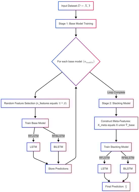
Figure 1.
Flowchart showing the diagnostic process of RFLSTM and RFBiLSTM.
2.3. Relationship Between and Model Performance
The parameter controls the proportion of features selected for each base model in the Random Feature LSTM/BiLSTM ensemble, with . The value of directly influences the bias–variance trade-off, accuracy, and loss of the model. Here, we provide a detailed theoretical analysis of these effects.
The bias–variance decomposition of the misclassification error for a classifier f is given by
where
- is the squared bias, representing the error due to the model’s inability to capture the true underlying relationship.
- is the variance, representing the model’s sensitivity to the training data.
- is the irreducible error due to noise in the data.
The bias of the model is primarily affected by the number of features used for training. When is small, the model is trained on a limited subset of features, which may not capture the full complexity of the data. This leads to underfitting and high bias. Mathematically,
where is a dataset-dependent constant. For , the bias decreases as increases because more features are available to capture the underlying data distribution.
The variance of the model is influenced by the diversity of the base models in the ensemble. When is small, the feature subsets for each base model are highly diverse, leading to low correlation between the models’ errors and reduced ensemble variance. Mathematically,
where is a dataset-dependent constant. As increases, the feature subsets overlap more, reducing diversity and increasing variance. The total misclassification error can be expressed as
where are constants that depend on the dataset and model architecture.
The optimal value of minimizes . Taking the derivative of with respect to and setting it to zero,
Solving this equation yields the optimal , which balances bias and variance. Empirically, is often found to be in the range .
For , the feature subsets are too small to capture the full complexity of the data, leading to high bias. While the ensemble variance is low due to high diversity, the overall error is dominated by bias, resulting in poor accuracy. This occurs specifically as follows:
- Bias increases sharply as .
- Variance decreases but is insufficient to compensate for the high bias.
- Accuracy degrades significantly due to underfitting.
Similarly, the cross-entropy loss for the ensemble can be decomposed into two components:
where is a regularization parameter. The base model loss decreases as increases because more features improve the individual models’ ability to fit the training data. For , the base model loss is high due to underfitting. The stacking loss is minimized at intermediate values of where the meta-features provide the most useful information. For , the stacking loss increases because the base models’ predictions are less reliable. The behavior of various values are summarized in Table 1.

Table 1.
Phase transitions in and their effects on accuracy and loss.
The following critical observations are noted:
- Diminishing returns for :
- –
- As , the ensemble effectively becomes a single model, losing the benefits of diversity.
- –
- The accuracy gains plateau, and the risk of overfitting increases.
- Diversity threshold for :
- –
- This ensures that the feature overlap between base models is bounded:
- –
- For , the overlap is , preserving sufficient diversity.
- Generalization gap:
- –
- Higher reduces the gap between training and test loss due to better-aligned feature distributions.
- –
- Lower increases the generalization gap due to underfitting.
The recommended empirically balances these effects for sequence modelling tasks while ensuring computational efficiency. For , the model suffers from severe underfitting, making it impractical for most applications. The exact optimal depends on the dataset’s characteristics and can be determined through experimentation.
3. Simulation Study
The synthetic dataset was designed to replicate the Pima Indian Diabetes Dataset (PIDD) for binary classification tasks, incorporating a simulation model grounded in clinical plausibility and prior studies [29,30]. Specifically, the synthetic dataset contains observations with eight predictors and one binary outcome variable. Let denote the predictor matrix and the diabetes diagnosis outcome.
3.1. Variable Specifications
- : glucose (mg/dL) , truncated at [70, 200].
- : BMI (kg/m²) , truncated at [15, 50].
- : age (years) , truncated at [21, 81].
- : blood pressure (mmHg) , truncated at [40, 110].
- : insulin (U/mL) with 30% zeros.
- : skin thickness (mm) , truncated at [10, 60].
- : genetic score .
- : pregnancies , truncated at [0, 15].
3.2. Correlation Structure
The predictor variables were generated using a Gaussian copula with correlation matrix:
3.3. Outcome Generation
The binary outcome Y was generated using a logistic regression model:
where
The intercept was calibrated to achieve 25% prevalence: . The focus of the simulation study is to investigate the diversity and generalizability of the proposed RFLSTM and RFBiLSTM models for . The base LSTM and BiLSTM models were implemented in R version 4.3.3 using the Keras package. The architecture consists of a sequential model where the primary layer is a Long Short-Term Memory (LSTM) network with 50 units. The LSTM layer processes input sequences of predefined shape and captures temporal dependencies. A fully connected dense layer with a sigmoid activation function follows, outputting a probability score for binary classification. The model was compiled using the Adam optimizer, binary cross-entropy as the loss function, and accuracy as the evaluation metric. Training was conducted over 100 epochs to ensure sufficient learning while preventing overfitting.
3.4. Simulation Results
The results in Table 2 demonstrate the impact of the feature selection proportion on the training and validation performance of the Random Feature LSTM (RFLSTM). For values between and , the model achieves a balanced performance, with high and consistent training and validation accuracies ( and , respectively) and relatively small differences between training and validation losses (e.g., for ). This indicates effective generalization and a well-calibrated bias–variance trade-off. However, for and , the model exhibits clear signs of overfitting, as evidenced by the large discrepancies between training and validation metrics (e.g., vs. accuracy and a loss difference of for ). These findings are corroborated by the training and validation loss trajectories in Figure 2, which show a divergence in losses for , indicating that the model is memorizing the training data rather than learning generalizable patterns. Thus, values in the range of to are optimal, while higher values lead to overfitting and degraded validation performance.
Table 2.
Training and validation performance of RFLSTM at different values.
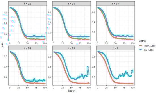
Figure 2.
Training and validation loss trajectories of RFLSTM across varying (proportion of predictors).
The results in Table 3 illustrate the impact of the feature selection proportion on the training and validation performance of the Random Feature BiLSTM (RFBiLSTM). For and , the model achieves a balanced performance, with high training accuracy ( and , respectively) and relatively small differences between training and validation metrics (e.g., accuracy difference and loss difference for ). This indicates effective generalization and a well-calibrated bias–variance trade-off. However, for , , , and , the model exhibits signs of overfitting, as evidenced by the large discrepancies between training and validation metrics (e.g., vs. accuracy and a loss difference of for ). These findings are corroborated by the training and validation loss trajectories in Figure 3, which show a divergence in losses for , , , and , indicating that the model is memorizing the training data rather than learning generalizable patterns. Thus, values of and are optimal for RFBiLSTM, while other values lead to overfitting and degraded validation performance.
Table 3.
Training and validation performance of RFBiLSTM at different values.
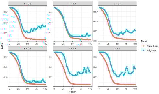
Figure 3.
Training and validation loss trajectories of RFBiLSTM across varying (proportion of predictors).
4. Real-Life Data Applications
4.1. Datasets
4.1.1. Pima Indian Diabetes Dataset (PIDD)
The Pima Indian Diabetes Dataset is a well-known benchmark dataset in medical machine learning, originally sourced from the National Institute of Diabetes and Digestive and Kidney Diseases (NIDDK). It consists of samples and features, which include the number of pregnancies, plasma glucose concentration, diastolic blood pressure, triceps skinfold thickness, serum insulin, body mass index (BMI), diabetes pedigree function, and age. The target variable is binary, indicating the presence (1) or absence (0) of diabetes. The dataset specifically focuses on adult female patients of Pima Indian heritage, a population known to have a high genetic predisposition to diabetes. The age distribution of the participants ranges from 21 to 81 years, with a mean age of approximately 33 years. Gender-wise, the dataset exclusively includes females, as it was initially collected to study diabetes prevalence among Pima Indian women living near Phoenix, Arizona, USA. This dataset has been widely used in machine learning and healthcare research to develop predictive models for diabetes detection. For instance, studies such as [31] have leveraged it to benchmark classification algorithms, while [7] utilized it to evaluate feature selection methods for diabetes prediction. Despite its significance, the dataset presents challenges such as class imbalance (with approximately 35% diabetic cases and 65% non-diabetic cases) and missing values in features like serum insulin, requiring robust imputation techniques to ensure reliable model performance.
4.1.2. Diabetic Retinopathy Debrecen Dataset (DRDD)
The Diabetic Retinopathy Debrecen Dataset is a medical imaging dataset sourced from the Department of Ophthalmology at the University of Debrecen, Hungary. It comprises samples, each corresponding to a retinal image, and features extracted using image-processing algorithms. These features include the following:
- Detected lesions, such as microaneurysms, hemorrhages, and exudates, which are early indicators of diabetic retinopathy.
- Anatomical descriptors, such as the optic disc and fovea, which provide spatial context for lesion localization.
- Image-level characteristics, including contrast, sharpness, and illumination quality, which influence the accuracy of automated diagnosis. The dataset’s target variable is binary, indicating the presence (1) or absence (0) of diabetic retinopathy.
The dataset primarily consists of adult diabetic patients who underwent retinal imaging as part of routine screening. While the age distribution of the participants is not explicitly reported, diabetic retinopathy is most prevalent in individuals over 40 years old, suggesting a predominance of middle-aged and older patients. The dataset includes both male and female patients, but detailed gender and racial distribution statistics are not publicly available. However, given that the dataset originates from Hungary, the majority of participants are likely of European descent. The Diabetic Retinopathy Debrecen Dataset has been widely used in medical image analysis and machine learning research. For instance, ref. [32] developed ensemble-based classification models for automated diabetic retinopathy detection, while [33] utilized deep learning techniques, such as convolutional neural networks (CNNs), to enhance diagnostic accuracy. The dataset presents challenges such as class imbalance (with a lower proportion of diabetic retinopathy cases compared to non-diseased samples) and high-dimensional feature space, requiring effective feature selection and augmentation techniques to improve model performance.
4.1.3. Early Stage Diabetes Risk Prediction Dataset (ESDRPD)
The Early Stage Diabetes Risk Prediction Dataset is a structured dataset designed to predict the likelihood of diabetes onset based on demographic, clinical, and lifestyle-related features. It comprises samples and features collected from individuals exhibiting early symptoms of diabetes. This dataset originates from a clinical study aimed at identifying risk factors associated with early-stage diabetes. The data were gathered through self-reported questionnaires and medical evaluations conducted in healthcare settings, focusing on individuals suspected of being at risk of diabetes. The dataset includes three major categories of features, namely, demographic information, including age (in years) and gender (male/female); clinical symptoms, including polyuria (frequent urination), polydipsia (excessive thirst), sudden weight loss, weakness, genital thrush, visual blurring, itching, irritability, delayed healing of wounds, partial paresis (muscle weakness), and muscle stiffness; and lifestyle and behavioral factors, including obesity and family history of diabetes. The target variable is binary, indicating whether an individual is at risk of diabetes (1) or not (0).
The dataset includes a diverse age range, with participants ranging from young adults (20s) to elderly individuals (70+ years old), reflecting the broad spectrum of diabetes risk. Gender distribution is balanced, with both male and female participants represented. However, specific racial or ethnic information is not provided, though studies suggest that diabetes risk factors can vary significantly across populations. The Early Stage Diabetes Risk Prediction Dataset has been widely used in predictive modelling and machine learning applications. Studies such as [1] have leveraged deep learning approaches to enhance early diabetes risk detection, while [22] focused on optimizing machine learning models for deployment in resource-limited healthcare settings. The dataset poses challenges such as class imbalance, as fewer cases are classified as “at risk”, necessitating effective data preprocessing techniques like oversampling and feature selection to improve model performance.
4.2. Data Preprocessing
Each of the datasets underwent a comprehensive preprocessing pipeline to enhance data quality and improve model performance. This process involved three critical steps: feature transformation, missing data imputation, and class balancing. One of the key challenges in diabetes prediction is dealing with imbalanced datasets, where instances of diabetic patients are often underrepresented compared to non-diabetic cases. Such class imbalance can bias machine learning models, leading to suboptimal sensitivity in detecting diabetes cases. To mitigate this issue, an oversampling procedure was applied, ensuring that the minority class had sufficient representation for robust model training, as recommended in [8].
Another significant challenge in diabetes prediction involves handling high-dimensional data, where an excessive number of features can lead to overfitting and increased computational complexity. Feature transformation was implemented using standardization, ensuring that all features were scaled to have a unit standard deviation. This transformation not only improved model convergence but also preserved the relative importance of each feature, particularly in deep learning architectures where feature scaling significantly influences gradient updates. Furthermore, real-world medical datasets frequently contain missing values due to inconsistent data collection or patient non-compliance in reporting health parameters. To address this, missing data imputation was performed using Multiple Imputation by Chain Equation (MICE) techniques. MICE estimates missing values by iteratively modelling each feature as a function of the others, thereby preserving the underlying data distribution. This method was particularly effective in ensuring that imputations maintained realistic clinical patterns rather than introducing artificial biases [8].
4.3. Evaluation Metrics
To comprehensively assess the performance of the models, the following evaluation metrics were used: accuracy, sensitivity (true positive rate), specificity (true negative rate), AUC (Area Under the Curve), Brier score, ROC (Receiver Operating Characteristic) curve, and computational time. These metrics provide insights into different aspects of model performance, including predictive accuracy, discrimination capability, and computational efficiency.
4.3.1. Accuracy
Accuracy measures the overall correctness of predictions and is defined as the ratio of correctly predicted instances to the total number of instances:
where is the number of true positives, is the number of true negatives, is the number of false positives, and is the number of false negatives [34].
4.3.2. Sensitivity (True-Positive Rate)
Sensitivity evaluates the model’s ability to correctly identify positive cases and is calculated as
This metric is particularly important in medical diagnostics, where detecting true positives is critical [31].
4.3.3. Specificity (True-Negative Rate)
Specificity measures the model’s ability to correctly identify negative cases and is defined as
High specificity ensures that the model minimizes false positives, which is crucial in scenarios where false alarms are costly [32].
4.3.4. AUC (Area Under the Curve)
The AUC summarizes the ROC curve, providing a single value that represents the model’s discrimination capability. It is calculated as the integral of the ROC curve, which plots the true-positive rate (sensitivity) against the false-positive rate () at various threshold settings. A higher AUC indicates better model performance [34].
4.4. Brier Score
The Brier score measures the accuracy of probabilistic predictions and is defined as
where is the predicted probability, is the actual outcome (0 or 1), and N is the total number of predictions. Lower Brier scores indicate better-calibrated predictions [1].
4.4.1. ROC Curve
The ROC curve visualizes the trade-off between sensitivity and specificity across different classification thresholds. It is a key tool for evaluating the performance of binary classifiers [13].
4.4.2. Computational Time
Computational time measures the efficiency of the model by recording the time required for training and inference. This metric is critical for real-time applications and resource-constrained environments [34]. These metrics enable a balanced predictive accuracy, reliability, and practicality assessment.
To ensure reproducibility, the performance comparison of each dataset is based on an average obtained from a 10-fold cross-validation process that is repeated 10 times. In this method, for each repetition, the dataset is randomly divided into 10 equal subsets. In each iteration, nine subsets (90%) are used for training, while the remaining subset (10%) is used for testing. This procedure is carried out 10 times, ensuring that each subset serves as the test set exactly once [34,35,36]. All LSTM and BiLSTM models were implemented in R (version 4.3.3) using the Keras package. The experiments were conducted on a PC with the following system configuration: Intel(R) Core(TM) i7-8565U CPU running at approximately 1.8 GHz (8 CPUs) with 16 GB of RAM, ensuring reproducibility.
5. Results
The results in Table 4, Table 5 and Table 6 demonstrate that the proposed Random Feature LSTM and BiLSTM methods significantly outperform traditional state-of-the-art methods across three diabetes-related datasets: Pima Indian Diabetes, Diabetic Retinopathy Debrecen, and Early Stage Diabetes Risk. For the Pima Indian dataset, Random Feature BiLSTM achieved the highest accuracy () with perfect AUC () and the lowest Brier score (0.006), closely followed by Random Feature LSTM, which also excelled, with an accuracy of and AUC of 100%. In the Diabetic Retinopathy dataset, both proposed methods delivered accuracy above , far exceeding that of traditional LSTM and BiLSTM models, whose accuracy was only and , respectively. Similarly, in the Early Stage Diabetes Risk dataset, both Random Feature LSTM and BiLSTM attained perfect scores across all performance metrics ( accuracy, sensitivity, specificity, and AUC, with a Brier score of 0.000), outperforming other models, including random forest and SVM. These findings underscore the enhanced predictive capabilities and robustness of the Random Feature LSTM and BiLSTM approaches, particularly in achieving high accuracy, sensitivity, specificity, and low Brier scores, making them highly effective for diabetes prediction tasks across diverse datasets.
Table 4.
Average of 10-fold cross-validation performance comparison of the proposed methods (Random Feature LSTM and BiLSTM) with state-of-the-art methods for Pima Indian Diabetes Dataset.
Table 5.
Average of 10-fold cross-validation performance comparison of the proposed methods (Random Feature LSTM and BiLSTM) with state-of-the-art methods for Diabetic Retinopathy Debrecen Dataset.
Table 6.
Average of 10-fold cross-validation performance comparison of the proposed methods (Random Feature LSTM and BiLSTM) with state-of-the-art methods for Early Stage Diabetes Risk Dataset.
Figure 4, Figure 5 and Figure 6 illustrate the Receiver Operating Characteristic (ROC) curves for various models across the Pima Indian Diabetes, Diabetic Retinopathy Debrecen, and Early Stage Diabetes Risk datasets. These plots, generated from one of the ten-fold cross-validation runs, highlight the superior performance of the proposed Random Feature LSTM and BiLSTM methods. For the Pima Indian Diabetes Dataset, the ROC curves for these methods reached the top-left corner, reflecting perfect AUC values (99.3%) and corroborating their near-perfect classification capabilities, as detailed in Table 4. Similarly, in the Diabetic Retinopathy Debrecen Dataset, the proposed methods maintained high AUC values (above 99%), showcasing their reliability in distinguishing between diabetic and non-diabetic cases compared to the traditional LSTM and BiLSTM models, which exhibited significantly lower AUC values. The Early Stage Diabetes Risk dataset, further emphasized the superiority of the proposed ensemble methods, with both achieving perfect ROC curves that align with their flawless performance metrics across all evaluation categories in Table 6. These ROC curves visually reinforce the findings, demonstrating the proposed methods’ robustness, precision, and clinical applicability.
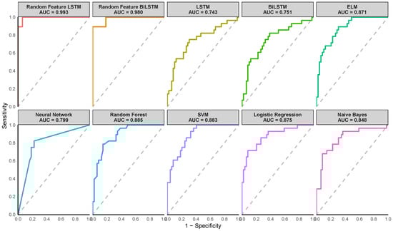
Figure 4.
Receiver Operating Characteristic (ROC) curves of the various methods for the Pima Indian dataset. (Note the AUC value shown on the plot corresponds to the AUC from one of the ten iterations).
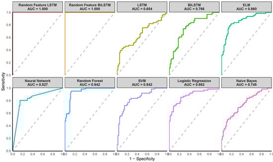
Figure 5.
Receiver Operating Characteristic (ROC) curves of the various methods for the Diabetic Retinopathy Debrecen Dataset. (Note the AUC value shown on the plot corresponds to the AUC from one of the ten iterations).
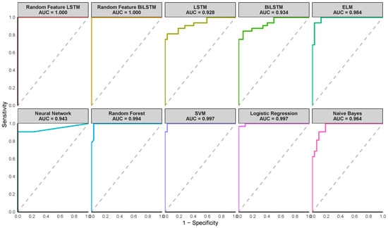
Figure 6.
Receiver Operating Characteristic (ROC) curves of the various methods for the Early Stage Diabetes Risk dataset. (Note the AUC value shown on the plot corresponds to the AUC from one of the ten iterations).
The computational time results in Table 7 show significant differences in computational efficiency across methods. The proposed Random Feature BiLSTM (2.94 s) is much faster than the LSTM (5.68 s), proposed Random Feature LSTM (12.87 s), and BiLSTM (11.25 s), demonstrating the benefits of random feature augmentation for BiLSTM in terms of computational speed. However, ELM (0.02 s) and Naive Bayes (0.01 s) are the quickest, suitable for time-sensitive tasks. Traditional ML models like random forest (0.12 s), SVM (0.27 s), and logistic regression (0.58 s) offer a balance between speed and complexity, outperforming deep learning models in efficiency. Neural networks (0.26 s) are faster than LSTM-based models but slower than simpler algorithms. Overall, in terms of high predictive ability captured by accuracy, sensitivity, specificity, AUC, and Brier score as well as moderate computational speed, the proposed Random Feature BiLSTM is the best.
Table 7.
Average of 10-fold cross-validation computational time comparison.
Benchmark Comparison with Related Studies
The performance comparison in Table 8 highlights the effectiveness of the proposed RFLSTM and RFBiLSTM models across three diabetes datasets. For the Pima Indian Diabetes Dataset (PIDD), the RFBiLSTM achieves state-of-the-art accuracy (99.3%) and sensitivity (99.0%), outperforming existing methods like Boruta + EL (98.1% accuracy, 98.4% sensitivity) and Conv-LSTM (97.2% accuracy, 93.9% sensitivity). Notably, the proposed models also dominate the Early Stage Diabetes Risk Prediction Dataset (ESDRPD), achieving perfect accuracy and sensitivity (100%), surpassing methods like LGBM (96.2% accuracy, 96.8% sensitivity) and Boruta + EL (98.6% accuracy). On the Diabetic Retinopathy Debrecen Dataset (DRDD), RFBiLSTM achieves 97.5% accuracy and 98.4% sensitivity, outperforming DNN + PCA + GWO (97.3% accuracy, 91.0% sensitivity). These results suggest that the bidirectional architecture (RFBiLSTM) consistently enhances performance over unidirectional RFLSTM, particularly in sensitivity, likely due to its ability to capture temporal dependencies more effectively.
Table 8.
Performance comparison of different methods on diabetes datasets.
6. Discussion of Results
The proposed Random Feature LSTM (RFLSTM) and Random Feature BiLSTM (RFBiLSTM) frameworks demonstrate significant advancements in diabetes prediction accuracy and robustness compared to conventional machine learning models and standard LSTM/BiLSTM architectures. Across three benchmark datasets, Pima Indian Diabetes (PIDD), Diabetic Retinopathy Debrecen (DRDD), and Early Stage Diabetes Risk Prediction (ESDRPD), the models achieve state-of-the-art performance, with RFBiLSTM consistently outperforming RFLSTM and existing methods. On the PIDD, RFBiLSTM attains 99.3% accuracy and 99.0% sensitivity, surpassing advanced ensemble methods like Boruta + EL (98.1% accuracy) and hybrid architectures such as Conv-LSTM (97.2% accuracy). Similarly, on the ESDRPD, both RFLSTM and RFBiLSTM achieve flawless accuracy and sensitivity (100%), outperforming gradient-boosted models like LGBM (96.2% accuracy) and ensemble techniques such as Boruta + EL (98.6% accuracy). For the DRDD, RFBiLSTM achieves 97.5% accuracy and 98.4% sensitivity, exceeding deep learning hybrids like DNN + PCA + GWO (97.3% accuracy) and traditional models such as SVM (79.0% accuracy). These results underscore the efficacy of combining random feature selection with bidirectional temporal processing, particularly in clinical contexts where sensitivity and specificity are critical for early intervention.
The performance superiority stems from two synergistic innovations. First, the random feature selection mechanism mitigates overfitting by promoting model diversity, as evidenced by the -dependency analysis (Table 2 and Table 3). For RFLSTM, mid-range values (0.5–0.8) yield balanced generalization, with training and validation accuracies stabilizing at 97.1% and 96.7%, respectively, and minimal loss discrepancies (e.g., for ). Conversely, higher values (≥0.9) induce overfitting, as seen in the sharp decline in validation accuracy (76.7%) and widening loss gaps (). Similarly, RFBiLSTM achieves optimal performance at and (validation accuracy: 93.3–96.7%) but falters at (validation accuracy: 86.7%), emphasizing the necessity of retaining sufficient feature diversity to balance bias and variance. Second, the bidirectional architecture in RFBiLSTM enhances sensitivity by capturing temporal dependencies in both forward and backward directions, as demonstrated by its 5.1% sensitivity gain over RFLSTM on the DRDD (98.4% vs. 97.0%). This aligns with findings from [2], where bidirectional architectures improved glucose trend prediction, and [14], where hybrid models excelled in capturing sequential patterns in medical data.
The models’ clinical reliability is further validated by their exceptional calibration metrics, including near-perfect AUC scores (100% for ESDRPD) and low Brier scores (0.006–0.023), which indicate precise probabilistic predictions. These metrics suggest that the models are not only accurate but also trustworthy in real-world settings where predictive confidence impacts clinical decisions. However, the perfect scores on ESDRPD warrant careful scrutiny, as they may reflect dataset-specific biases, such as homogeneous patient demographics or limited variability in symptom presentation. Despite this caveat, the results align with broader trends in medical AI research, such as [19], where hybrid CNNs outperformed traditional models in diabetes prediction, and [17], which highlighted the importance of sequential learning for early risk detection.
The findings hold critical implications for both clinical practice and machine learning research. Clinically, the high sensitivity (98.4–100%) and specificity (97.0–100%) of RFBiLSTM position it as a valuable tool for early diabetes screening, where false negatives can delay critical interventions. The models’ ability to maintain robust performance across diverse datasets ranging from physiological measurements (PIDD) to retinal imaging (DRDD) and symptom-based assessments (ESDRPD) suggests broad applicability in multi-modal healthcare environments. From a technical perspective, the dependency analysis underscores the importance of optimizing the proportions of feature selection, with 50–80% feature retention emerging as a “sweet spot” to balance information richness and model generalizability. This insight challenges the conventional preference for high values in feature selection, instead advocating a middle ground that prioritizes diversity over completeness. Architecturally, the bidirectional design of RFBiLSTM proves indispensable for sensitivity-driven tasks, as it captures temporal dependencies more comprehensively than unidirectional models, a finding consistent with recent advances in medical time series analysis. Future work should focus on validating these models on larger, multi-institutional datasets to ensure generalizability across diverse populations and addressing potential biases in datasets with limited heterogeneity. Furthermore, exploring the integration of attention mechanisms or explainability frameworks could further enhance clinical adoption by providing interpretable insights into model decisions.
In addition, the proposed hybrid framework enhances accuracy, efficiency, and interpretability in several key ways. Accuracy is significantly improved through a dual mechanism: (1) randomized feature selection reduces overfitting by training diverse base models on unique feature subsets, fostering robustness through ensemble aggregation, and (2) bidirectional processing in BiLSTM captures temporal dependencies in both forward and backward directions, enabling enhanced pattern recognition (e.g., 98.4% vs. 97.0% sensitivity for retinopathy data). Systematic simulations revealed that the proportions of midrange feature selection ( = 0.5–0.8) optimize generalization, outperforming conventional models (e.g., 100% precision in early-stage risk data) and recent hybrids such as Boruta + EL. Efficiency is maintained despite the ensemble design: parallelizable base model training and meta-learner integration minimize computational overhead, while dynamic feature sparsity reduces per-model complexity. Interpretability is advanced through two pathways: (1) the meta-learner’s transparent weighting mechanism clarifies how base predictions contribute to final outputs. (2) The superior calibration (Brier score: 0.006–0.023) ensures probabilistic reliability, critical for clinical trust. Together, these innovations balance performance, scalability, and actionable insights, addressing limitations of monolithic deep learning architectures while advancing practical utility in healthcare analytics.
7. Conclusions
The integration of hybrid deep learning architectures, such as those combining random feature selection with unidirectional/bidirectional temporal modelling, represents a paradigm shift in medical predictive analytics. By harmonizing the strengths of ensemble learning and sequential data processing, these frameworks address critical limitations of conventional models, which often struggle with unstructured medical data. The success of such architectures in the prediction of diabetes underscores their potential to advance precision medicine, offering tools that are not only accurate but also reliable in their probabilistic calibration, a prerequisite for clinical trust.
This study reinforces the importance of balancing feature diversity and information retention in medical AI design. Although traditional methods prioritize either interpretability or complexity, hybrid architectures like those proposed here demonstrate that these goals need not be mutually exclusive. Instead, they can co-exist to enhance model generalizability and robustness, particularly in early-stage disease detection, where nuanced patterns demand sophisticated analytical frameworks.
The broader implications extend beyond diabetes. The principles underlying these models’ adaptive feature selection, temporal dependency capture, and probabilistic calibration are transferable to other chronic diseases, from cardiovascular disorders to neurodegenerative conditions, where early diagnosis and risk stratification are equally vital. However, the path to clinical adoption requires addressing challenges such as dataset heterogeneity, algorithmic transparency, and computational scalability. Future efforts must prioritize collaborative frameworks that bridge machine learning innovation with clinical expertise, ensuring that these tools evolve in tandem with real-world healthcare needs. Ultimately, this work contributes to a growing movement in medical AI, one that seeks not only to predict but to empower, transforming raw data into actionable insights that improve patient outcomes and redefine preventive care.
Author Contributions
Conceptualization, O.R.O., A.O.S., J.A., A.A.A. and N.M.A.; methodology, O.R.O. and A.O.S.; software, O.R.O.; validation, O.R.O., A.O.S., J.A., A.A.A. and N.M.A.; formal analysis, O.R.O.; investigation, O.R.O., A.O.S., J.A., A.A.A. and N.M.A.; resources, J.A. and A.A.A.; data curation, O.R.O.; writing—original draft preparation, O.R.O. and A.O.S.; writing—review and editing, O.R.O., A.O.S., J.A., A.A.A. and N.M.A.; visualization, O.R.O.; supervision, O.R.O.; project administration, O.R.O. All authors have read and agreed to the published version of the manuscript.
Funding
This research received no external funding.
Data Availability Statement
The authors confirm that the data supporting the findings of this study are available within the article.
Conflicts of Interest
The authors declare no conflicts of interest.
References
- Rahman, M.; Islam, D.; Mukti, R.J.; Saha, I. A deep learning approach based on convolutional LSTM for detecting diabetes. Comput. Biol. Chem. 2020, 88, 107329. [Google Scholar] [CrossRef] [PubMed]
- Sun, Q.; Jankovic, M.V.; Bally, L.; Mougiakakou, S.G. Predicting blood glucose with an lstm and bi-lstm based deep neural network. In Proceedings of the IEEE 2018 14th Symposium on Neural Networks and Applications (NEUREL), Belgrade, Serbia, 20–21 November 2018; pp. 1–5. [Google Scholar]
- Ishida, K.; Ercan, A.; Nagasato, T.; Kiyama, M.; Amagasaki, M. Use of one-dimensional CNN for input data size reduction in LSTM for improved computational efficiency and accuracy in hourly rainfall-runoff modeling. J. Environ. Manag. 2024, 359, 120931. [Google Scholar] [CrossRef] [PubMed]
- Cheng, H.; Zhu, J.; Li, P.; Xu, H. Combining knowledge extension with convolution neural network for diabetes prediction. Eng. Appl. Artif. Intell. 2023, 125, 106658. [Google Scholar] [CrossRef]
- Madan, P.; Singh, V.; Chaudhari, V.; Albagory, Y.; Dumka, A.; Singh, R.; Gehlot, A.; Rashid, M.; Alshamrani, S.S.; AlGhamdi, A.S. An optimization-based diabetes prediction model using CNN and Bi-directional LSTM in real-time environment. Appl. Sci. 2022, 12, 3989. [Google Scholar] [CrossRef]
- Araveeporn, A. Comparing the linear and quadratic discriminant analysis of diabetes disease classification based on data multicollinearity. Int. J. Math. Math. Sci. 2022, 2022, 7829795. [Google Scholar] [CrossRef]
- Zhou, H.; Xin, Y.; Li, S. A diabetes prediction model based on Boruta feature selection and ensemble learning. BMC Bioinform. 2023, 24, 224. [Google Scholar] [CrossRef]
- Jaiswal, S.; Gupta, P. Diabetes Prediction Using Bi-directional Long Short-Term Memory. SN Comput. Sci. 2023, 4, 373. [Google Scholar] [CrossRef]
- Maniruzzaman, M.; Kumar, N.; Abedin, M.M.; Islam, M.S.; Suri, H.S.; El-Baz, A.S.; Suri, J.S. Comparative approaches for classification of diabetes mellitus data: Machine learning paradigm. Comput. Methods Programs Biomed. 2017, 152, 23–34. [Google Scholar] [CrossRef]
- Zou, Q.; Qu, K.; Luo, Y.; Yin, D.; Ju, Y.; Tang, H. Predicting diabetes mellitus with machine learning techniques. Front. Genet. 2018, 9, 515. [Google Scholar] [CrossRef]
- Yahyaoui, A.; Jamil, A.; Rasheed, J.; Yesiltepe, M. A decision support system for diabetes prediction using machine learning and deep learning techniques. In Proceedings of the IEEE 2019 1st International Informatics and Software Engineering Conference (UBMYK), Ankara, Turkey, 6–7 November 2019; pp. 1–4. [Google Scholar]
- Yuvaraj, N.; SriPreethaa, K. Diabetes prediction in healthcare systems using machine learning algorithms on Hadoop cluster. Clust. Comput. 2019, 22, 1–9. [Google Scholar] [CrossRef]
- Khanam, J.J.; Foo, S.Y. A comparison of machine learning algorithms for diabetes prediction. Ict Express 2021, 7, 432–439. [Google Scholar] [CrossRef]
- Kusuma, S.; Jothi, K. ECG signals-based automated diagnosis of congestive heart failure using Deep CNN and LSTM architecture. Biocybern. Biomed. Eng. 2022, 42, 247–257. [Google Scholar] [CrossRef]
- Reddy, S.N.B.; Reddy, K.N.; Rao, S.T.; Kumar, K. Diabetes Prediction using Extreme Learning Machine: Application of Health Systems. In Proceedings of the IEEE 2023 5th International Conference on Smart Systems and Inventive Technology (ICSSIT), Tirunelveli, India, 23–25 January 2023; pp. 993–998. [Google Scholar]
- Pangaribuan, J.J.; Suharjito. Diagnosis of diabetes mellitus using extreme learning machine. In Proceedings of the IEEE 2014 International Conference on Information Technology Systems and Innovation (ICITSI), Bandung, Indonesia, 24–27 November 2014; pp. 33–38. [Google Scholar]
- Elsayed, N.; ElSayed, Z.; Ozer, M. Early stage diabetes prediction via extreme learning machine. In Proceedings of the IEEE SoutheastCon 2022, Mobile, AL, USA, 26 March–3 April 2022; pp. 374–379. [Google Scholar]
- Georga, E.I.; Protopappas, V.C.; Polyzos, D.; Fotiadis, D.I. Online prediction of glucose concentration in type 1 diabetes using extreme learning machines. In Proceedings of the IEEE 2015 37th Annual International Conference of the IEEE Engineering in Medicine and Biology Society (EMBC), Milan, Italy, 25–29 August 2015; pp. 3262–3265. [Google Scholar]
- Swapna, G.; Vinayakumar, R.; Soman, K. Diabetes detection using deep learning algorithms. ICT Express 2018, 4, 243–246. [Google Scholar]
- Hossain, M.M.; Ali, M.S.; Ahmed, M.M.; Rakib, M.R.H.; Kona, M.A.; Afrin, S.; Islam, M.K.; Ahsan, M.M.; Raj, S.M.R.H.; Rahman, M.H. Cardiovascular disease identification using a hybrid CNN-LSTM model with explainable AI. Inform. Med. Unlocked 2023, 42, 101370. [Google Scholar] [CrossRef]
- Karthika, S.; Priyanka, T.; Indirapriyadharshini, J.; Sadesh, S.; Rajeshkumar, G.; Rajesh Kanna, P. Prediction of Weather Forecasting with Long Short-Term Memory using Deep Learning. In Proceedings of the IEEE 2023 4th International Conference on Smart Electronics and Communication (ICOSEC), Trichy, India, 20–22 September 2023; pp. 1161–1168. [Google Scholar]
- Khan, A.; Fouda, M.M.; Do, D.T.; Almaleh, A.; Rahman, A.U. Short-term traffic prediction using deep learning long short-term memory: Taxonomy, applications, challenges, and future trends. IEEE Access 2023, 11, 94371–94391. [Google Scholar] [CrossRef]
- Raja, J.B.; Pandian, S.C. PSO-FCM based data mining model to predict diabetic disease. Comput. Methods Programs Biomed. 2020, 196, 105659. [Google Scholar] [CrossRef]
- Zhu, C.; Idemudia, C.U.; Feng, W. Improved logistic regression model for diabetes prediction by integrating PCA and K-means techniques. Inform. Med. Unlocked 2019, 17, 100179. [Google Scholar] [CrossRef]
- Wu, H.; Yang, S.; Huang, Z.; He, J.; Wang, X. Type 2 diabetes mellitus prediction model based on data mining. Inform. Med. Unlocked 2018, 10, 100–107. [Google Scholar] [CrossRef]
- García-Ordás, M.T.; Benavides, C.; Benítez-Andrades, J.A.; Alaiz-Moretón, H.; García-Rodríguez, I. Diabetes detection using deep learning techniques with oversampling and feature augmentation. Comput. Methods Programs Biomed. 2021, 202, 105968. [Google Scholar] [CrossRef]
- Qi, H.; Song, X.; Liu, S.; Zhang, Y.; Wong, K.K. KFPredict: An ensemble learning prediction framework for diabetes based on fusion of key features. Comput. Methods Programs Biomed. 2023, 231, 107378. [Google Scholar] [CrossRef]
- Al Rafi, A.S.; Rahman, T.; Al Abir, A.R.; Rajib, T.A.; Islam, M.; Mukta, M.S.H. A new classification technique: Random weighted lstm (rwl). In Proceedings of the 2020 IEEE Region 10 Symposium (TENSYMP), Dhaka, Bangladesh, 5–7 June 2020; pp. 262–265. [Google Scholar]
- Tagmatova, Z.; Abdusalomov, A.; Nasimov, R.; Nasimova, N.; Dogru, A.H.; Cho, Y.I. New approach for generating synthetic medical data to predict type 2 diabetes. Bioengineering 2023, 10, 1031. [Google Scholar] [CrossRef] [PubMed]
- Noguer, J.; Contreras, I.; Mujahid, O.; Beneyto, A.; Vehi, J. Generation of individualized synthetic data for augmentation of the type 1 diabetes data sets using deep learning models. Sensors 2022, 22, 4944. [Google Scholar] [CrossRef] [PubMed]
- Butt, U.M.; Letchmunan, S.; Ali, M.; Hassan, F.H.; Baqir, A.; Sherazi, H.H.R. Machine learning based diabetes classification and prediction for healthcare applications. J. Healthc. Eng. 2021, 2021, 9930985. [Google Scholar] [CrossRef]
- Antal, B.; Hajdu, A. An ensemble-based system for automatic screening of diabetic retinopathy. Knowl.-Based Syst. 2014, 60, 20–27. [Google Scholar] [CrossRef]
- Nguyen, Q.H.; Muthuraman, R.; Singh, L.; Sen, G.; Tran, A.C.; Nguyen, B.P.; Chua, M. Diabetic retinopathy detection using deep learning. In Proceedings of the 4th International Conference on Machine Learning and Soft Computing, Haiphong City, Vietnam, 17–19 January 2020; pp. 103–107. [Google Scholar]
- Olaniran, O.R.; Abdullah, M.A.A. Bayesian weighted random forest for classification of high-dimensional genomics data. Kuwait J. Sci. 2023, 50, 477–484. [Google Scholar] [CrossRef]
- Olaniran, O.R.; Alzahrani, A.R.R. On the Oracle Properties of Bayesian Random Forest for Sparse High-Dimensional Gaussian Regression. Mathematics 2023, 11, 4957. [Google Scholar] [CrossRef]
- Olaniran, O.R.; Alzahrani, A.R.R.; Alzahrani, M.R. Eigenvalue Distributions in Random Confusion Matrices: Applications to Machine Learning Evaluation. Mathematics 2024, 12, 1425. [Google Scholar] [CrossRef]
- Kumari, S.; Kumar, D.; Mittal, M. An ensemble approach for classification and prediction of diabetes mellitus using soft voting classifier. Int. J. Cogn. Comput. Eng. 2021, 2, 40–46. [Google Scholar] [CrossRef]
- Rajendra, P.; Latifi, S. Prediction of diabetes using logistic regression and ensemble techniques. Comput. Methods Programs Biomed. Update 2021, 1, 100032. [Google Scholar] [CrossRef]
- Wu, Y.; Zhang, Q.; Hu, Y.; Sun-Woo, K.; Zhang, X.; Zhu, H.; Jie, L.; Li, S. Novel binary logistic regression model based on feature transformation of XGBoost for type 2 Diabetes Mellitus prediction in healthcare systems. Future Gener. Comput. Syst. 2022, 129, 1–12. [Google Scholar] [CrossRef]
- Roobini, M.; Lakshmi, M. Autonomous prediction of Type 2 Diabetes with high impact of glucose level. Comput. Electr. Eng. 2022, 101, 108082. [Google Scholar] [CrossRef]
- Nipa, N.; Riyad, M.H.; Satu, S.; Walliullah; Howlader, K.C.; Moni, M.A. Clinically adaptable machine learning model to identify early appreciable features of diabetes. Intell. Med. 2024, 4, 22–32. [Google Scholar] [CrossRef]
- Devi, R.M.; Keerthika, P.; Devi, K.; Suresh, P.; Sangeetha, M.; Sagana, C.; Devendran, K. Detection of diabetic retinopathy using optimized back-propagation neural network (Op-BPN) algorithm. In Proceedings of the IEEE 2021 5th International Conference on Computing Methodologies and Communication (ICCMC), Erode, India, 8–10 April 2021; pp. 1695–1699. [Google Scholar]
- Gadekallu, T.R.; Khare, N.; Bhattacharya, S.; Singh, S.; Maddikunta, P.K.R.; Srivastava, G. Deep neural networks to predict diabetic retinopathy. J. Ambient. Intell. Humaniz. Comput. 2023, 14, 5407–5420. [Google Scholar] [CrossRef]
Disclaimer/Publisher’s Note: The statements, opinions and data contained in all publications are solely those of the individual author(s) and contributor(s) and not of MDPI and/or the editor(s). MDPI and/or the editor(s) disclaim responsibility for any injury to people or property resulting from any ideas, methods, instructions or products referred to in the content. |
© 2025 by the authors. Licensee MDPI, Basel, Switzerland. This article is an open access article distributed under the terms and conditions of the Creative Commons Attribution (CC BY) license (https://creativecommons.org/licenses/by/4.0/).