Using Machine Learning for the Precise Experimental Modeling of Catastrophe Phenomena: Taking the Establishment of an Experimental Mathematical Model of a Cusp-Type Catastrophe for the Zeeman Catastrophe Machine as an Example

Abstract

When catastrophe theory is applied to the experimental modeling of catastrophe phenomena, it is impossible to know in advance the corresponding relationship and mapping form between the parameters of the actual catastrophe mathematical model and the parameters of the canonical catastrophe mathematical model. This gives rise to the problem in which the process of experimental modeling cannot be completed in many instances. To solve this problem, an experimental modeling method of catastrophe theory is proposed. It establishes the quantitative relationship between the actual catastrophe mathematical model and the canonical catastrophe mathematical model by assuming that the actual potential function is equal to the canonical potential function, and it uses a machine learning model to represent the diffeomorphism that can realize the error-free transformation of the two models. The method is applied to establish the experimental mathematical model of a cusp-type catastrophe for the Zeeman catastrophe machine. Through programming calculation, it is found that the prediction errors of the potential function, manifold, and bifurcation set of the established model are 0.0455%, 0.0465%, and 0.1252%, respectively. This indicates that the established model can quantitatively predict the catastrophe phenomenon.

1. Introduction

Catastrophic phenomena refer to the sudden shifts in a system’s state that occur in various fields due to strong nonlinearities in the system. Since the occurrence of catastrophe phenomena has a great influence on the development process of items, research on catastrophe phenomena, especially the control and utilization of catastrophe phenomena, is of great significance in controlling the development direction and the final results of items [1,2,3].

Establishing a relatively precise mathematical model is the basis and key to the control and utilization of catastrophe phenomena. Catastrophe theory [4] is a tool to establish the mathematical model of catastrophe phenomena. In the more than 50 years since the establishment of catastrophe theory, people [5,6,7,8,9] have used the modeling method provided by it to establish various mathematical models for a large number of catastrophe phenomena, and the mathematical models have been used to control and utilize the catastrophe phenomena, achieving a lot of results. In the existing research, some inherent defects and congenital problems of the modeling method for catastrophe theory have also attracted people’s attention. One of the problems that has the greatest impact on the application development of the precise modeling of catastrophe phenomena and the modeling methods of catastrophe theory, and that people are most interested in solving, is the following: except for a few special cases [10,11,12], the actual (experimental) catastrophe mathematical models established by using experimental observation data of the catastrophe phenomena are qualitative (analog) models that do not have the ability to perform quantitative prediction, and it is difficult for these models to meet the requirements of precise control and rational utilization of catastrophe phenomena. In fact, this is the “practical efficiency problem” [13] of catastrophe theory, which greatly limits its application scope and quality. Because of the existence of this problem, the academic community participated in a far-reaching debate on supporting and opposing the catastrophe theory at the beginning of the creation of the catastrophe theory [14,15]. In the face of doubt, Thom [16] openly admitted that “catastrophe theory is fundamentally a qualitative explanatory theory, which itself has no predictive ability” and “in a sense, it can be called analogy theory”. Unfortunately, to this day, this problem has not been resolved.

The root cause of the problem is as follows: when using the modeling method of catastrophe theory, especially the “experimental modeling method” [17], which is considered by the founder of the catastrophe theory to be the most promising method to establish a catastrophe mathematical model, the corresponding relationship and mapping form between the actual parameters (the actual control and state parameters used to represent the actual catastrophe mathematical model) and the canonical parameters (the canonical control and state parameters used to represent the canonical catastrophe mathematical model) are very complex and have strong nonlinear characteristics. However, the founder of the catastrophe theory did not inform the corresponding relationship and mapping form in advance and did not provide an effective method to determine them. It can only be subjectively set by the modeler based on experience. To deal with the problem conveniently, almost all researchers set the corresponding relationship between the actual parameters and the canonical parameters as a one-to-one correspondence, and they set the mapping form between them as a simple proportional function, linear function [18], or polynomial function [19]. For example, the manifold of the cusp-type catastrophe mathematical model is directly written as “$4x^3+2aux+bv=0$” [20] or “$x^3+2aux+bv=0$” [21] ($x$ is the canonical state parameter; $u$ and $v$ are the canonical control parameters; and $a$ and $b$ are the proportional coefficients between the actual parameters and the canonical parameters) and so on. The fact that it is difficult to make the artificially determined corresponding relationship and mapping form be completely consistent with the real situation results in unforeseen and, in many cases, large prediction errors in the catastrophe mathematical models that have been established. When the prediction error exceeds a certain range, the ability of the models to make quantitative predictions is lost.

So, how can the complex correspondence and mapping relationship (nonlinear relationship) between the actual parameters and the canonical parameters be expressed and obtained accurately?

As we all know, the machine learning model [22] established by experimental observation data has a strong ability to characterize and simulate the complex nonlinear relationship between data points. Therefore, it is a natural choice for people to use machine learning to solve the above problem. Zheng et al. [23] established a machine learning model by using the random forest algorithm and the experimental data of chip bifurcation catastrophe and realized the accurate prediction of chip bifurcation phenomenon. The prediction accuracy, precision, and recall rate of whether the chip bifurcation phenomenon occurs under the condition of given control parameters reached 100%. Li et al. [24] used an RBF neural network trained with simulation data to simulate the mapping between the canonical control parameters ($u$,$v$) and the actual control parameters (Reynolds number $Re$ and angle of attack $\alpha$) to modify the experimental modeling method of catastrophe theory. Using the modified experimental modeling method, the prediction error (compared to the simulation value) of the bifurcation set of the cusp-type catastrophe mathematical model for the airfoil-stall boundary at a low Reynolds number was reduced to less than 1%. Unfortunately, the modified experimental modeling method and related techniques are only used to improve the prediction accuracy of the bifurcation set in the specific catastrophe mathematical model, but not to improve the prediction accuracy of the potential function and the manifold of the catastrophe mathematical model. Daw et al. 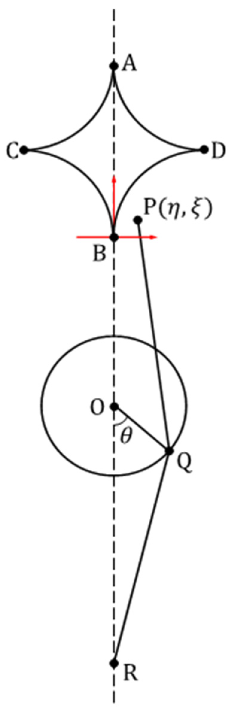[25] used a mixture density neural network to simulate the bimodal (upper and lower leaves of the manifold) of the statistical mathematical model of a cusp-type catastrophe based on statistical catastrophe theory and achieved a successful result. When the machine learning model was experimentally verified using three previously established datasets of the Zeeman catastrophe machine [26] (a mechanism, as shown in Figure 1, hereinafter referred to as “ZCM”), it was found that the root mean square errors (loss function values) of the two-component mixture density neural network were 0.10, 0.20, and 0.79, respectively.

So far, there has been no report on the use of machine learning technology to completely solve the above problem in the experimental modeling method.

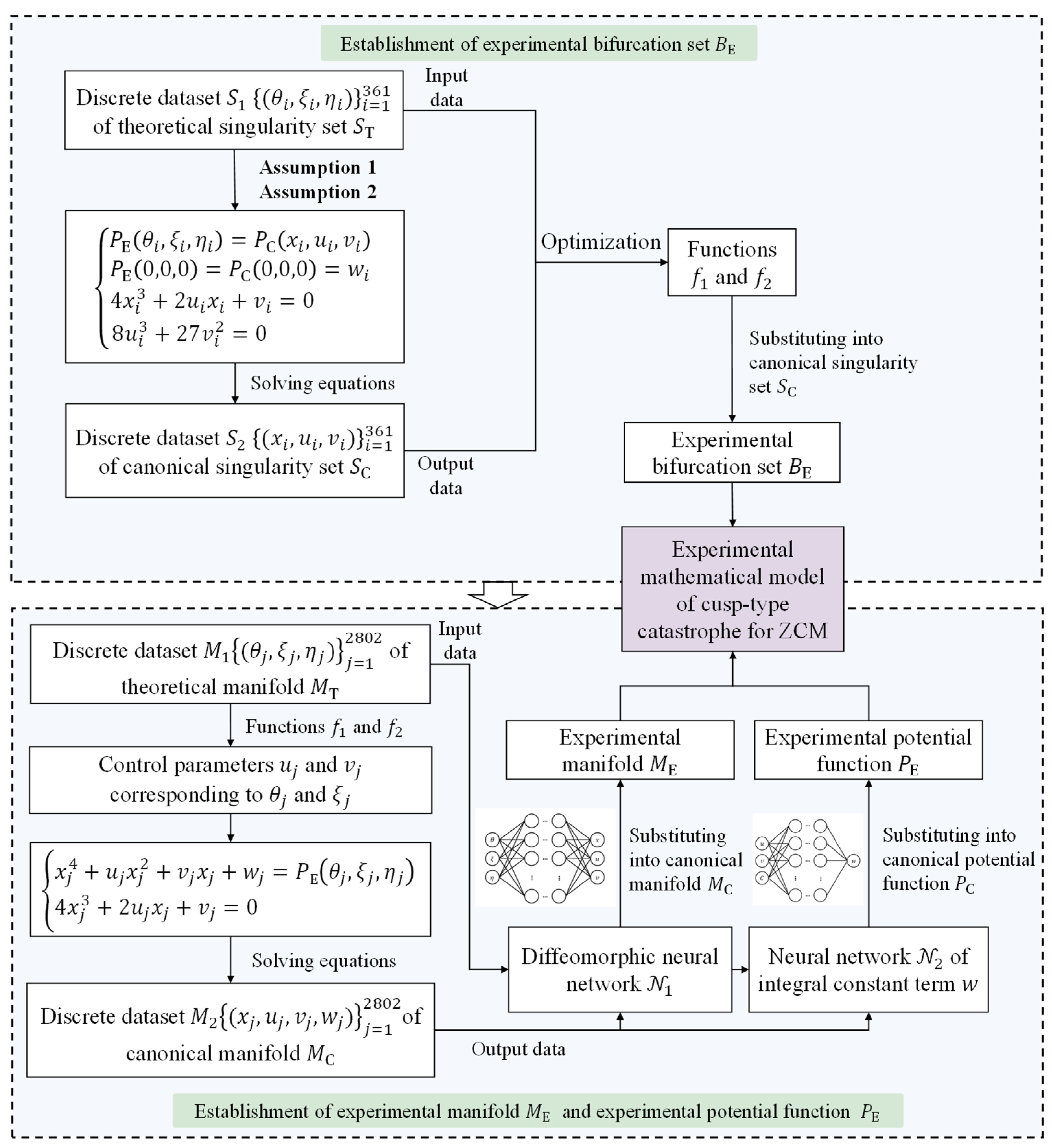
In this paper, we propose a method of precise experimental modeling of catastrophe phenomena using experimental datasets of a singularity set and manifold, which establishes the quantitative relationship between the experimental catastrophe mathematical model and the canonical catastrophe mathematical model by assuming that the experimental potential function is equal to the canonical potential function, and then we determine the diffeomorphism [27] represented by a machine learning model that can achieve error-free transformations of the two models. Taking the precise experimental modeling of a cusp-type catastrophe for ZCM as an example, the key points and implementation results of this method are explained. Through programming calculation, it is found that the prediction errors of the potential function, manifold, and bifurcation set of the experimental mathematical model of a cusp-type catastrophe for ZCM are 0.0309%, 0.0650%, and 0.1252%, respectively. This indicates that the established model has the ability to quantitatively predict the catastrophe phenomenon.

2. Establishment of Experimental Mathematical Model of Cusp-Type Catastrophe for ZCM

2.1. Introduction to ZCM

The ZCM (Figure 1) is an instructional device invented by the British mathematician Zeeman to verify the validity of conclusions related to catastrophe theory [26]. This device played an irreplaceable role in the development of catastrophe theory and holds significant academic and historical value.

Anyone familiar with the history of catastrophe theory knows that the widespread acceptance, dissemination, and application of the theory owe much to the ZCM. Years ago, Zeeman spent several weeks personally constructing this simple mechanical demonstration model, which allowed him to clearly illustrate the process of catastrophe phenomena, their characteristic signatures, and their objective existence. This demonstration convincingly validated the correctness of catastrophe theory, earning it broad recognition.

Since then, many researchers working on catastrophe theory and its applications have used the ZCM as a primary physical model to evaluate their proposed methods or validate their research findings. It is generally believed that if a method can effectively analyze and handle the ZCM, it largely meets the requirements of catastrophe theory.

Therefore, in this study, we take the establishment of an experimental mathematical model of a cusp-type catastrophe for the ZCM as an example to illustrate the key aspects of the proposed method and its implementation results.

2.2. Establishment of Experimental Dataset

As mentioned above, in order to use machine learning technology to establish the experimental mathematical model of a cusp-type catastrophe for the ZCM, it is necessary to obtain the experimental dataset of the singularity set and the manifold of ZCM.

The accuracy of the ZCM, which can only be manufactured by hand, is hard to ensure, leading to a larger error in the experimental dataset obtained through real test experiments. To enhance modeling accuracy, the experimental dataset required for modeling is obtained by discretizing the singularity set and manifold of the theoretical mathematical model of a cusp-type catastrophe for the ZCM established by previous researchers.

2.2.1. Theoretical Mathematical Model of Cusp-Type Catastrophe for ZCM Established by Previous Researchers

The theoretical mathematical model of a cusp-type catastrophe for the ZCM established by Poston et al. [17] through theoretical analysis is

$$\left\{\begin{array}{c}{P}_{\mathrm{T}}\left(\theta ,\xi ,\eta \right)={\displaystyle \frac{1}{2}}\mu \left[{\left(r_1-1\right)}^2+{\left(r_2-1\right)}^2\right] \\ M_{\mathrm{T}}:{\displaystyle \frac{\partial P_{\mathrm{T}}\left(\theta ,\xi ,\eta \right)}{\partial \theta }}=0 \\ S_{\mathrm{T}}:{\displaystyle \frac{{\partial }^2{P}_{\mathrm{T}}\left(\theta ,\xi ,\eta \right)}{\partial {\theta }^2}}=0 \\ B_{\mathrm{T}}:\left\{\begin{array}{c}{\displaystyle \frac{\partial P_{\mathrm{T}}\left(\theta ,\xi ,\eta \right)}{\partial \theta }}=0\\ {\displaystyle \frac{{\partial }^2{P}_{\mathrm{T}}\left(\theta ,\xi ,\eta \right)}{\partial {\theta }^2}}=0\end{array}\right.\stackrel{Eliminate \theta }{\Rightarrow }b\left(\xi ,\eta \right)=0\end{array}\right.$$

(1)

where $P_{\mathrm{T}}\left(\theta ,\xi ,\eta \right)$ is the theoretical potential function of the theoretical mathematical model of a cusp-type catastrophe for the ZCM; $\theta$ is the actual state parameter; $\xi$ and $\eta$ are the actual control parameters; $\mu$, $r_1$, and $r_2$ are the performance and structural parameters of ZCM; $M_{\mathrm{T}}$ is the theoretical manifold; $S_{\mathrm{T}}$ is the theoretical singularity set; and $B_{\mathrm{T}}$ is the theoretical bifurcation set.

2.2.2. Establishment of Discrete Dataset S₁ of Theoretical Singularity Set S_T

The value interval ($-\pi /2, \pi /2$) of the actual state parameter $\theta$ is discretized in an equal interval manner. If the discrete interval is $\pi /360$, then 361 $\theta$ values are obtained, denoted by ${\theta }_i$ ($i=1,2,\cdots 361$).

By substituting ${\theta }_i$ into $\left\{\begin{array}{c}{\displaystyle \frac{\partial P_{\mathrm{T}}\left(\theta ,\xi ,\eta \right)}{\partial \theta }}=0\\ {\displaystyle \frac{{\partial }^2{P}_{\mathrm{T}}\left(\theta ,\xi ,\eta \right)}{\partial {\theta }^2}}=0\end{array}\right.$ in Equation (1), the binary system of equations about $({\xi }_i,{\eta }_i)$ is obtained. By solving the binary system of equations numerically, the coordinates $({\xi }_i,{\eta }_i)$ of discrete control points corresponding to ${\theta }_i$ on the theoretical bifurcation set $B_{\mathrm{T}}$ are obtained.

${\left\{({\theta }_i,{\xi }_i,{\eta }_i)\right\}}_{i=1}^{361}$ is the discrete dataset $S_1$ of the theoretical singularity set $S_{\mathrm{T}}$, as shown in

Table 1. Discrete dataset S₁ of theoretical singularity set S_T.

$\mathit{i}$	${\mathit{\theta }}_{\mathit{i}}$	${\mathit{\xi }}_{\mathit{i}}$	${\mathit{\eta }}_{\mathit{i}}$
1	−1.5708	0.4668	0.7035
2	−1.5621	0.4671	0.7021
3	−1.5533	0.4674	0.7007
4	−1.5446	0.4678	0.6992
5	−1.5359	0.4681	0.6977
$⋮$	$⋮$	$⋮$	$⋮$
$⋮$	$⋮$	$⋮$	$⋮$
$⋮$	$⋮$	$⋮$	$⋮$
360	1.5621	0.4671	−0.7021
361	1.5708	0.4668	−0.7035

.

2.2.3. Establishment of Discrete Dataset M₁ of Theoretical Manifold M_T

The control plane is discretized in a given region ($\xi \in \left(0, 0.5\right),\eta \in \left(-1, 1\right)$) with rectangular grids with side lengths of ${∆}_1=0.0080$ and ${∆}_2=0.0400$, respectively. The coordinates of the discrete grid nodes $({\xi }_j,{\eta }_j)$ are substituted into the theoretical manifold $M_{\mathrm{T}}$ to obtain a univariate equation about ${\theta }_j$. In this way, the phase point coordinates ${\theta }_j$ corresponding to $({\xi }_j,{\eta }_j)$ can be obtained by solving the univariate equation.

${\left\{({\theta }_j,{\xi }_j,{\eta }_j)\right\}}_{j=1}^{2802}$ is the discrete dataset $M_1$ of the theoretical manifold $M_{\mathrm{T}}$, as shown in

Table 2. Discrete dataset M₁ of theoretical manifold M_T.

$\mathit{j}$	${\mathit{\theta }}_{\mathit{j}}$	${\mathit{\xi }}_{\mathit{j}}$	${\mathit{\eta }}_{\mathit{j}}$
1	1.0190	0.0082	1.0000
2	1.0028	0.0082	0.9592
3	0.9866	0.0082	0.9184
4	0.9703	0.0082	0.8776
5	0.9538	0.0082	0.8367
$⋮$	$⋮$	$⋮$	$⋮$
$⋮$	$⋮$	$⋮$	$⋮$
$⋮$	$⋮$	$⋮$	$⋮$
2801	1.3661	0.4673	0.5510
2802	1.3601	0.4673	0.5102

.

2.3. Modeling Assumptions

According to the catastrophe theory, the canonical mathematical model of a cusp-type catastrophe is

$$\left\{\begin{array}{c}{P}_{\mathrm{C}}\left(x,u,v\right)=x^4+u{x}^2+vx+w \\ M_{\mathrm{C}}:{\displaystyle \frac{\partial P_{\mathrm{C}}\left(x,u,v\right)}{\partial x}}=4x^3+2ux+v=0 \\ S_{\mathrm{C}}:{\displaystyle \frac{{\partial }^2{P}_{\mathrm{C}}\left(x,u,v\right)}{\partial x^2}}=6x^2+u=0 \\ B_{\mathrm{C}}:\left\{\begin{array}{c}{\displaystyle \frac{\partial P_{\mathrm{C}}\left(x,u,v\right)}{\partial x}}=0\\ {\displaystyle \frac{{\partial }^2{P}_{\mathrm{C}}\left(x,u,v\right)}{\partial x^2}}=0\end{array}\right.\stackrel{Eliminate x}{\Rightarrow }8u^3+27v^2=0\end{array}\right.$$

(2)

where $P_{\mathrm{C}}\left(x,u,v\right)$ is the canonical potential function of the canonical mathematical model of a cusp-type catastrophe, $x$ is the canonical state parameter, $u$ and $v$ are the canonical control parameters, $w$ is an integral constant term independent of the canonical state parameter $x$, $M_{\mathrm{C}}$ is the canonical manifold, $S_{\mathrm{C}}$ is the canonical singularity set, and $B_{\mathrm{C}}$ is the canonical bifurcation set.

It is important to note the following: (1) The canonical mathematical model is the fundamental mathematical model in catastrophe theory. It has a standardized form and comprehensive content, serving as a crucial foundation for constructing experimental catastrophe mathematical models for specific phenomena. (2) Compared to the canonical catastrophe model, an experimental mathematical model of catastrophe is derived from experimental data and describes the catastrophic behavior of a specific phenomenon. Any experimental mathematical model of catastrophe expressed in terms of actual parameters can be transformed into a canonical catastrophe model through a diffeomorphism between actual and theoretical parameters.

As mentioned above, in order to use the above experimental dataset and the canonical mathematical model of a cusp-type catastrophe to establish the experimental mathematical model of a cusp-type catastrophe for the ZCM, it is necessary to first establish the quantitative correspondence between the experimental mathematical model of a cusp-type catastrophe for the ZCM and the canonical mathematical model of a cusp-type catastrophe.

Considering that the experimental mathematical model of a cusp-type catastrophe for the ZCM is obtained by the error-free diffeomorphism transformation of the canonical mathematical model of a cusp-type catastrophe, the potential function values at the corresponding phase points before and after the transformation should be equal. The following assumption is made:

Assumption 1. 

The potential function $P_E\left(\theta ,\xi ,\eta \right)$ of the experimental mathematical model of a cusp-type catastrophe for the ZCM is equal to the canonical potential function $P_C\left(x,u,v\right)$.

Taking into account that the canonical potential function is the universal unfolding 2 of the singularity, which is the simplest form of the versal unfolding 2 of the singularity, and in order to simplify the subsequent calculation process, the following assumption is made:

Assumption 2. 

The origin of the singularity set of the experimental mathematical model of a cusp-type catastrophe for the ZCM coincides with the origin of the singularity set of the canonical mathematical model of a cusp-type catastrophe, so the potential function values corresponding to these two origins are equal.

Figure 2 depicts the entire modeling process. The detailed modeling process and key points will be revealed in Section 2.4, Section 2.5 and Section 2.6.

2.4. Establishment of Experimental Bifurcation Set $B_E$

The specific process and steps of establishing the experimental bifurcation set $B_{\mathrm{E}}$ of the experimental mathematical model of a cusp-type catastrophe for the ZCM are as follows:

(1)

Calculate the discrete dataset S₂ of the canonical singularity set S_C corresponding to the discrete dataset S₁.

It can be seen from Assumption 1 that the potential function values at the matching points on the actual singularity set $S_{\mathrm{E}}$ and the canonical singularity set $S_{\mathrm{C}}$ are equal, that is,

$$P_{\mathrm{E}}\left({\theta }_i,{\xi }_i,{\eta }_i\right)=P_{\mathrm{C}}\left(x_i,u_i,v_i\right),i=1,2,\cdots 361$$

(3)

From Assumption 2, it is evident that the origin of the actual singularity set $S_{\mathrm{E}}$ coincides with the origin of the canonical singularity set $S_{\mathrm{C}}$, so the potential function values corresponding to these two origins are equal, that is,

$$P_{\mathrm{E}}\left(0,0,0\right)=P_{\mathrm{C}}\left(0,0,0\right)=w_i,i=1,2,\cdots 361$$

(4)

It can be seen from the catastrophe theory that the coordinates $\left(x_i,u_i,v_i\right)$ of any point (such as point $i$) on the canonical singularity set $S_{\mathrm{C}}$ satisfy the canonical manifold $M_{\mathrm{C}}$, that is,

$$4x_i^3+2u_i{x}_i+v_i=0$$

(5)

The points on the bifurcation set are the projection of the singularity set on the control plane, so their coordinates $\left(x_i,u_i,v_i\right)$ should also satisfy the canonical bifurcation set $B_{\mathrm{C}}$, that is,

$$8u_i^3+27v_i^2=0$$

(6)

By combining Equations (3)–(6), a quaternary system of equations for $x_i$, $u_i$, $v_i$, and $w_i$ is obtained. Note that ${\theta }_i$, ${\xi }_i$, and ${\eta }_i$ are known in the system of equations, and the remaining four unknowns are $x_i$, $u_i$, $v_i$, and $w_i$. By solving the system of equations, the coordinates $\left(x_i,u_i,v_i\right)$ of the points of the canonical singularity set $S_{\mathrm{C}}$ that match the coordinates $\left({\theta }_i,{\xi }_i,{\eta }_i\right)$ of the points of the theoretical singularity set $S_{\mathrm{T}}$ can be obtained. Equation (4) indicates that the integral constant term $w_i$ is a constant value.

${\left\{(x_i,u_i,v_i)\right\}}_{i=1}^{361}$ is the discrete dataset $S_2$ of the canonical singularity set $S_{\mathrm{C}}$, as shown in

Table 3. Matching results of singularity set.

$\mathit{i}$	${\mathit{\theta }}_{\mathit{i}}$	${\mathit{\xi }}_{\mathit{i}}$	${\mathit{\eta }}_{\mathit{i}}$	${\mathit{x}}_{\mathit{i}}$	${\mathit{u}}_{\mathit{i}}$	${\mathit{v}}_{\mathit{i}}$
1	−1.5708	0.4668	0.7035	−0.7140	−3.0585	−2.9115
2	−1.5621	0.4671	0.7021	−0.7138	−3.0573	−2.9099
3	−1.5533	0.4674	0.7007	−0.7137	−3.0561	−2.9082
4	−1.5446	0.4678	0.6992	−0.7135	−3.0549	−2.9064
5	−1.5359	0.4681	0.6977	−0.7134	−3.0535	−2.9045
$⋮$	$⋮$	$⋮$	$⋮$	$⋮$	$⋮$	$⋮$
$⋮$	$⋮$	$⋮$	$⋮$	$⋮$	$⋮$	$⋮$
$⋮$	$⋮$	$⋮$	$⋮$	$⋮$	$⋮$	$⋮$
360	1.5621	0.4671	−0.7021	0.7138	−3.0573	2.9099
361	1.5708	0.4668	−0.7035	0.7140	−3.0585	2.9115

.

(2)

Determine the form of functions between the actual control parameters $(\xi ,\eta )$ and the canonical control parameters $(u,v)$.

To determine the functions between the actual control parameters $(\xi ,\eta )$ and the canonical control parameters $(u,v)$, we must first determine its form. It is well known that any function can be approximated by a polynomial, and the higher the degree of the polynomial, the better the approximation effect. After many attempts, it is found that setting the functions as a cubic polynomial and a higher polynomial does not significantly increase the accuracy of the experimental mathematical model of a cusp-type catastrophe for the ZCM to be established, that is, setting the functions as a quadratic polynomial can meet the requirements, namely,

$$\left\{\begin{array}{c}u=f_1\left(\xi ,\eta \right)={\displaystyle \sum _{k_1^1,k_2^1}^{k_1^1+k_2^1\le 2}}{p}_{k_1^1,k_2^1}{\xi }^{k_1^1}{\eta }^{k_2^1}\in \mathbb{R}\left[\xi ,\eta \right]\\ v=f_2\left(\xi ,\eta \right)={\displaystyle \sum _{k_1^2,k_2^2}^{k_1^2+k_2^2\le 2}}{q}_{k_1^2,k_2^2}{\xi }^{k_1^2}{\eta }^{k_2^2}\in \mathbb{R}\left[\xi ,\eta \right]\end{array}\right.$$

(7)

where $f_1$ and $f_2$ are the functions between the actual control parameters $(\xi ,\eta )$ and the canonical control parameters $(u,v)$ expressed in polynomial form; $k_1^1$, $k_2^1$, $k_1^2$, and $k_2^2$ are the exponents of polynomials, and $k_1^1,k_2^1,k_1^2,k_2^2\in \left\{0,1,2\right\}$; and $p_{k_1^1,k_2^1}\in \mathbb{R}$ and $q_{k_1^2,k_2^2}\in \mathbb{R}$ are 12 undetermined coefficients, and their values are generally determined by experimental dataset and optimization techniques.

(3)

Determine the undetermined coefficients of the functions f₁ and f₂.

Construct the following function:

$$g\left(\mathit{P},\xi ,\eta ,u,v\right)={\left[u-f_1\left(\xi ,\eta \right)\right]}^2+{\left[v-f_2\left(\xi ,\eta \right)\right]}^2$$

(8)

where $\mathit{P}$ is the function coefficient vector, $\mathit{P}=(p_{k_1^1,k_2^1},q_{k_1^2,k_2^2})$.

By substituting the coordinate $({\xi }_i,{\eta }_i)(i=1,2,\cdots 361)$ of the actual control points corresponding to the discrete dataset $S_1$ and the coordinate $(u_i,v_i)(i=1,2,\cdots 361)$ of the canonical control points corresponding to the discrete dataset $S_2$ into Equation (8), 361 functions about the coefficient vector $\mathit{P}$ are obtained, that is,

$$g_i\left(\mathit{P},{\xi }_i,{\eta }_i,u_i,v_i\right)={\left[u_i-f_1\left({\xi }_i,{\eta }_i\right)\right]}^2+{\left[v_i-f_2\left({\xi }_i,{\eta }_i\right)\right]}^2,i=1,2,\cdots 361$$

(9)

Construct the unconstrained optimization objective function as follows:

$$\underset{\mathit{P}}{\mathrm{m}\mathrm{i}\mathrm{n}} F=\underset{\mathit{P}}{\mathrm{m}\mathrm{i}\mathrm{n}}\sum _{i=1}^m{g}_i\left(\mathit{P},{\xi }_i,{\eta }_i,u_i,v_i\right)$$

(10)

The 1stOpt mathematical optimization toolkit is used to obtain all the undetermined coefficients $\mathit{P}$ when $F$ is minimized, as shown in

Table 4. Solution results of undetermined coefficients of function $f_1$ and $f_2$.

Function	Variable	Coefficient	Estimation
$f_1$	Constant	$p_{0,0}$	−0.2778
	$\xi$	$p_{1,0}$	−7.9098
	$\eta$	$p_{0,1}$	$-8.6819\times {10}^{-10}$
	${\xi }^2$	$p_{2,0}$	7.0926
	$\xi \eta$	$p_{1,1}$	$1.8938\times {10}^{-9}$
	${\eta }^2$	$p_{0,2}$	−1.3532
$f_2$	Constant	$q_{0,0}$	$2.8529\times {10}^{-6}$
	$\xi$	$q_{1,0}$	$-2.5793\times {10}^{-5}$
	$\eta$	$q_{0,1}$	−14.7025
	${\xi }^2$	$q_{2,0}$	$4.9709\times {10}^{-5}$
	$\xi \eta$	$q_{1,1}$	21.7942
	${\eta }^2$	$q_{0,2}$	$-4.2682\times {10}^{-6}$

.

As shown in Table 4, the dependent variable $u$ in $f_1$ is not correlated with the independent variables $\eta$ and $\xi \eta$, while the dependent variable $v$ in $f_2$ is only correlated with $\eta$ and $\xi \eta$. After removing the irrelevant terms, the final forms of $f_1$ and $f_2$ are determined as follows:

$$\left\{\begin{array}{c}u=f_1\left(\xi ,\eta \right)=p_{0,0}+p_{1,0}\xi +p_{2,0}{\xi }^2+p_{0,2}{\eta }^2\\ v=f_2\left(\xi ,\eta \right)=q_{0,1}\eta +q_{1,1}\xi \eta \end{array}\right.$$

(11)

The regression coefficients corresponding to the solution results are R = 0.9966 and R = 0.9966, respectively.

Substituting the coefficients obtained from Table 4 into Equation (11) yields the desired functions $f_1$ and $f_2$.

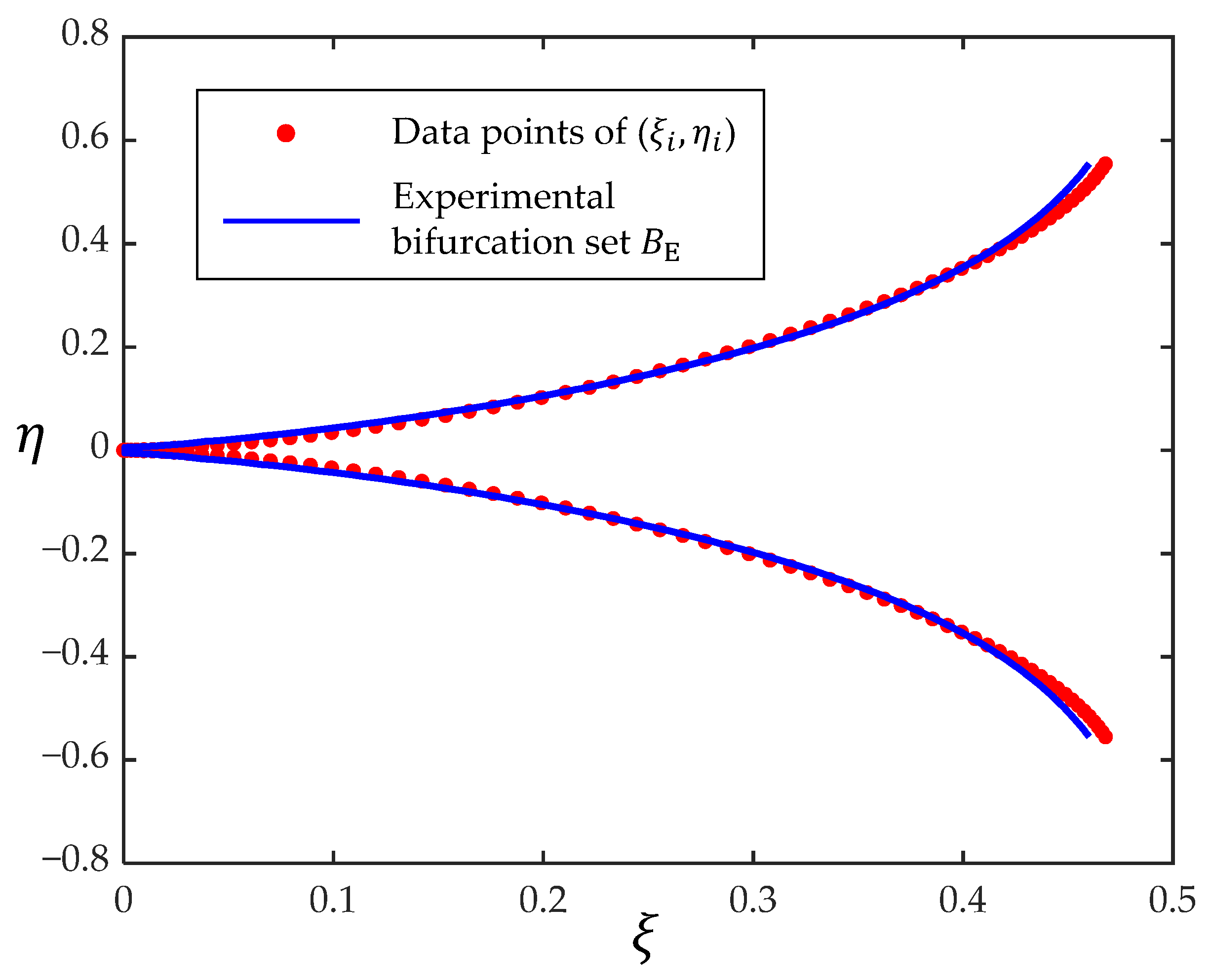
According to the canonical bifurcation set $B_{\mathrm{C}}$, the experimental bifurcation set $B_{\mathrm{E}}$ (Figure 3) is

$$8{(p_{0,0}+p_{1,0}\xi +p_{2,0}{\xi }^2+p_{0,2}{\eta }^2)}^3+27{(q_{0,1}\eta +q_{1,1}\xi \eta )}^2=0$$

(12)

2.5. Establishment of Experimental Manifold $M_E$

The specific process and steps of establishing the experimental manifold $M_{\mathrm{E}}$ of the experimental mathematical model of a cusp-type catastrophe for the ZCM are as follows:

(1)

Calculate the discrete dataset M₂ of the canonical manifold M_C that matches the discrete dataset M₁.

By substituting the actual control parameters ${\xi }_j$ and ${\eta }_j$ into the functions $f_1$ and $f_2$, the corresponding canonical control parameters $u_j$ and $v_j$ are obtained. By substituting $u_j$ and $v_j$ into Equation (5), a cubic equation about $x_j$ is obtained. By solving it, 1~3 real roots are obtained, that is, 1~3 canonical state parameters $x_j$ are obtained. According to the catastrophe theory, if three roots are solved, one of them corresponds to the maximum value of the potential function, which belongs to the unstable equilibrium point, and the corresponding system state cannot be obtained. The other two roots correspond to the two minimum values of the potential function, that is, the two stable equilibrium points of the system, and their symbols are opposite. One of these two roots with the same symbol as ${\theta }_j$ is taken as the canonical state parameter $x_j$ corresponding to ${\theta }_j$.

${\left\{(x_j,u_j,v_j)\right\}}_{j=1}^{2802}$ is the discrete dataset $M_2$ of the canonical manifold $M_{\mathrm{C}}$, as shown in

Table 5. Matching results of manifold.

$\mathit{j}$	${\mathit{\theta }}_{\mathit{j}}$	${\mathit{\xi }}_{\mathit{j}}$	${\mathit{\eta }}_{\mathit{j}}$	${\mathit{x}}_{\mathit{j}}$	${\mathit{u}}_{\mathit{j}}$	${\mathit{v}}_{\mathit{j}}$	${\mathit{w}}_{\mathit{j}}$
1	1.0190	0.0082	1.0000	1.7201	−1.6951	−14.5246	21.8528
2	1.0028	0.0082	0.9592	1.6896	−1.5869	−13.9317	20.5177
3	0.9866	0.0082	0.9184	1.6589	−1.4832	−13.3389	19.2252
4	0.9703	0.0082	0.8776	1.6278	−1.3840	−12.7460	17.9745
5	0.9538	0.0082	0.8367	1.5963	−1.2893	−12.1532	16.7649
$⋮$	$⋮$	$⋮$	$⋮$	$⋮$	$⋮$	$⋮$	$⋮$
$⋮$	$⋮$	$⋮$	$⋮$	$⋮$	$⋮$	$⋮$	$⋮$
$⋮$	$⋮$	$⋮$	$⋮$	$⋮$	$⋮$	$⋮$	$⋮$
2801	1.3661	0.4673	0.5510	1.3685	−2.8362	−2.4890	6.1460
2802	1.3601	0.4673	0.5102	1.3477	−2.7776	−2.3046	5.7866

.

(2)

Determine the diffeomorphism between the actual parameters $(\theta ,\xi ,\eta )$ and the canonical parameters $(x,u,v)$.

As is well known, neural networks can approximate functions of arbitrary complexity with any desired precision [28]. Therefore, in this study, a fully connected neural network is employed to model the diffeomorphic mapping between the actual parameters $(\theta ,\xi ,\eta )$ and the canonical parameters $(x,u,v)$. The mathematical proof demonstrating that a fully connected neural network can realize diffeomorphic transformations is provided in Appendix A.

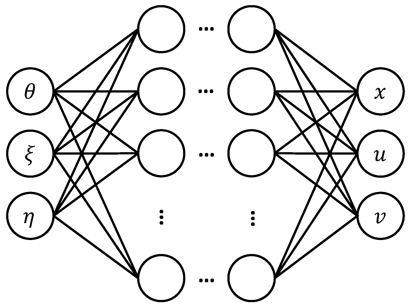
On the MATLAB R2023a platform, a fully connected neural network ${\mathcal{N}}_1$ is constructed to approximate diffeomorphic mapping, with the actual parameters $(\theta ,\xi ,\eta )$ as inputs and the canonical parameters $(x,u,v)$ as outputs, as shown in Figure 4. In a neural network ${\mathcal{N}}_1$, both the hidden layers and the output layer utilize the sigmoid activation function, while the mean squared error (MSE) is adopted as the loss function. The training dataset ${\{\left({\theta }_k,{\xi }_k,{\eta }_k\right),(x_k,u_k,v_k\left)\right\}}_{k=1}^{3163}$ is derived from the computational results in Table 3 and Table 5.

The Bayesian optimization algorithm [29] is employed to optimize the hyperparameters of the neural network model, including the number of hidden layers, the number of neurons per hidden layer, the learning rate, and the early stopping patience [30]. During optimization, the five-fold cross-validation error is used as the objective function for Bayesian optimization to prevent overfitting. The optimization results of the model are presented in

Table 6. Optimized hyperparameters of ${\mathcal{N}}_1$ using Bayesian optimization algorithm.

Hyperparameters	Optimal Value
Number of hidden layers	2
Number of neurons in hidden layers	28, 17
Learning rate	0.0015
Early stopping patience (avoid overfitting)	14

.

By retraining the neural network ${\mathcal{N}}_1$ with the optimized hyperparameters, it is observed that the regression coefficients for the training set, validation set, test set, and overall dataset all exceed 0.9998, indicating an excellent regression performance (Figure 5). The trained neural network is then saved and denoted as $\left[x,u,v\right]=sim(net1,\left[\theta ,\xi ,\eta \right])$.

According to the canonical manifold $M_{\mathrm{C}}$, the experimental manifold $M_{\mathrm{E}}$ is

$$4x^3+2ux+v=0$$

(13)

where $\left[x,u,v\right]=sim(net1,\left[\theta ,\xi ,\eta \right])$.

2.6. Establishment of Experimental Potential Function P_E

The specific process and steps of establishing the experimental potential function $P_{\mathrm{E}}$ of the experimental mathematical model of a cusp-type catastrophe for the ZCM are as follows:

(1)

Calculate the value of the integral constant term of the canonical potential function.

Substitute the discrete dataset $M_1$ and its matching $M_2$ into the theoretical potential function $P_{\mathrm{T}}$ and the canonical potential function $P_{\mathrm{C}}$ with the integral constant term removed, respectively, and calculate the value of the integral constant term $w_j$ corresponding to each discrete point:

$$w_j=P_{\mathrm{T}}\left({\theta }_j,{\xi }_j,{\eta }_j\right)-\left(x_j^4+u_j{x}_j^2+v_j{x}_j\right), j=1,2,\cdots 2802$$

(14)

The calculation results are shown in Table 6.

(2)

Determine the neural network ${\mathcal{N}}_2$ of the integral constant term $w$ of the canonical potential function $P_{\mathrm{C}}$.

On the MATLAB software platform, a neural network ${\mathcal{N}}_2$ with $\left(u,v,C\right)$ as the input and $w$ as the output is built (Figure 6). Here, $C$ is the parameter that distinguishes the phase points $\left(u,v,x\right)$ at the upper and lower leaves of the manifold. When the phase point $\left(u,v,x\right)$ is located on the upper leaf of the manifold, $x\ge \sqrt{-u/6}$, $C=0$; when the phase point $\left(u,v,x\right)$ is located on the lower leaf of the manifold, $x\le -\sqrt{-u/6}$, $C=1$.

In a neural network ${\mathcal{N}}_2$, both the hidden layers and the output layer use the sigmoid activation function, with the mean squared error (MSE) being used as the loss function. The training dataset ${\{\left(u_j,v_j,C_j\right),w_j\}}_{j=1}^{2802}$ is derived from the computational results in Table 5.

The Bayesian optimization algorithm [29] is used to optimize the hyperparameters of the neural network model. During optimization, the five-fold cross-validation error is employed as the objective function for Bayesian optimization. The optimization results of the model are shown in

Table 7. Optimized hyperparameters of ${\mathcal{N}}_2$ using Bayesian optimization algorithm.

Hyperparameters	Optimal Value
Number of hidden layers	2
Number of neurons in hidden layers	36, 21
Learning rate	0.0007
Early stopping patience (avoid overfitting)	5

.

By retraining the neural network ${\mathcal{N}}_2$ with the optimized hyperparameters, it is found that the regression coefficients for the training set, validation set, test set, and overall dataset all exceed 0.9998, demonstrating excellent regression performance (Figure 7). The trained neural network is then saved and denoted as $w=sim(net2,\left[u,v,C\right])$.

According to the canonical potential function $P_{\mathrm{C}}$, the experimental potential function $P_{\mathrm{E}}$ is

$$P_{\mathrm{E}}=x^4+u{x}^2+vx+w$$

(15)

where $\left[x,u,v\right]=sim(net1,\left[\theta ,\xi ,\eta \right])$; $w=sim(net2,\left[u,v,C\right])$.

Equations (12), (13) and (15) are combined to form the precise experimental mathematical model of a cusp-type catastrophe for the ZCM.

3. Prediction Errors of Experimental Mathematical Model of Cusp-Type Catastrophe for ZCM

3.1. Prediction Error of Experimental Potential Function $P_E$

The prediction error of the experimental potential function $P_{\mathrm{E}}$ is defined as the maximum absolute error of $P_{\mathrm{E}}$ relative to the true value (which is calculated by the theoretical potential function $P_{\mathrm{T}}$), namely,

$${∆}_P=\underset{\begin{array}{c}\theta \in \left(-\pi /2,\pi /2\right)\\ \begin{array}{c}\xi \in \left(0,0.5\right)\\ \eta \in \left(-1,1\right)\end{array}\end{array}}{\mathrm{m}\mathrm{a}\mathrm{x}}\left(\left|P_{\mathrm{T}}\left(\theta ,\xi ,\eta \right)-P_{\mathrm{E}}\left(\theta ,\xi ,\eta \right)\right|\right)=\left|P_{\mathrm{T}}\left({\theta }^{*},{\xi }^{*},{\eta }^{*}\right)-P_{\mathrm{E}}\left({\theta }^{*},{\xi }^{*},{\eta }^{*}\right)\right|\approx 0.0004$$

(16)

where $\left({\theta }^{\mathrm{*}},{\xi }^{\mathrm{*}},{\eta }^{\mathrm{*}}\right)=\underset{\begin{array}{c}\theta \in \left(-\pi /2,\pi /2\right)\\ \begin{array}{c}\xi \in \left(0,0.5\right)\\ \eta \in \left(-1,1\right)\end{array}\end{array}}{\mathrm{a}\mathrm{r}\mathrm{g}\mathrm{m}\mathrm{a}\mathrm{x}}\left(\left|P_{\mathrm{T}}\left(\theta ,\xi ,\eta \right)-P_{\mathrm{E}}\left(\theta ,\xi ,\eta \right)\right|\right)$ ≈ (0.4000, 0.6735, 1.3071), and the result of $\underset{\begin{array}{c}\theta \in \left(-\pi /2,\pi /2\right)\\ \begin{array}{c}\xi \in \left(0,0.5\right)\\ \eta \in \left(-1,1\right)\end{array}\end{array}}{\mathrm{a}\mathrm{r}\mathrm{g}\mathrm{m}\mathrm{a}\mathrm{x}}\left(\left|P_{\mathrm{T}}\left(\theta ,\xi ,\eta \right)-P_{\mathrm{E}}\left(\theta ,\xi ,\eta \right)\right|\right)$ is the corresponding variable point $\left({\theta }^{\mathrm{*}},{\xi }^{\mathrm{*}},{\eta }^{\mathrm{*}}\right)$ when $\left(\left|P_{\mathrm{T}}\left(\theta ,\xi ,\eta \right)-P_{\mathrm{E}}\left(\theta ,\xi ,\eta \right)\right|\right)$ reaches the maximum; $P_{\mathrm{T}}\left({\theta }^{\mathrm{*}},{\xi }^{\mathrm{*}},{\eta }^{\mathrm{*}}\right)$ ≈ 0.8787; $P_{\mathrm{E}}\left({\theta }^{\mathrm{*}},{\xi }^{\mathrm{*}},{\eta }^{\mathrm{*}}\right)$ ≈ 0.8783.

The corresponding relative error is

$${\delta }_P=\left|{\displaystyle \frac{{∆}_P}{P_{\mathrm{T}}\left({\theta }^{*},{\xi }^{*},{\eta }^{*}\right)}}\right|\times 100\%=\left|{\displaystyle \frac{P_{\mathrm{T}}\left({\theta }^{*},{\xi }^{*},{\eta }^{*}\right)-P_{\mathrm{E}}\left({\theta }^{*},{\xi }^{*},{\eta }^{*}\right)}{P_{\mathrm{T}}\left({\theta }^{*},{\xi }^{*},{\eta }^{*}\right)}}\right|\times 100\%\approx 0.0455\%$$

(17)

3.2. Prediction Error of Experimental Manifold $M_E$

It is important to note that the experimental manifold established $M_{\mathrm{E}}$ in Section 2.5 incorporates the neural network ${\mathcal{N}}_1$ and is only capable of mapping experimental data points $\left(\theta ,\xi ,\eta \right)$ onto the canonical manifold ${\mathrm{M}}_{\mathrm{C}}$. It cannot be used to directly compute the actual state parameter $\theta$ corresponding to specific control parameters $(\xi ,\eta )$. Therefore, we present a method for computing the actual state parameter $\theta$ based on the experimental manifold $M_{\mathrm{E}}$: (1) Substitute the actual control parameters $(\xi ,\eta )$ into the functions $f_1$ and $f_2$ to obtain the corresponding canonical control parameters $(u,v)$. Then, substitute $(u,v)$ into Equation (13) to derive a cubic equation in $x$. Solving this equation yields one to three real roots, corresponding to one to three canonical state parameters $x$. (2) On the MATLAB platform, a neural network ${\mathcal{N}}_3$ is constructed with $\left(x,u,v\right)$ as inputs and $\theta$ as the output. In ${\mathcal{N}}_3$, both the hidden layers and the output layer use the sigmoid activation function, and the mean squared error (MSE) is employed as the loss function. The training dataset ${\{\left(x_k,u_k,v_k\right),{\theta }_k\}}_{k=1}^{3163}$ is derived from the computational results in Table 3 and Table 5. The Bayesian optimization algorithm [29] is used to optimize the hyperparameters of the neural network model, with the five-fold cross-validation error serving as the objective function to prevent overfitting. The optimization results are presented in

Table 8. Optimized hyperparameters of ${\mathcal{N}}_3$ using Bayesian optimization algorithm.

Hyperparameters	Optimal Value
Number of hidden layers	2
Number of neurons in hidden layers	23, 35
Learning rate	0.0023
Early stopping patience (avoid overfitting)	9

. After retraining with the optimized hyperparameters, it is observed that the regression coefficients for the training set, validation set, test set, and overall dataset all exceed 0.9998, indicating excellent regression performance. The trained neural network is then saved and denoted as $\theta =sim(net3,\left[x,u,v\right])$. (3) By inputting the canonical parameters $\left(x,u,v\right)$ into the trained ${\mathcal{N}}_3$, the actual state parameter $\theta$ corresponding to the given control parameters $(\xi ,\eta )$ can be obtained.

The prediction error of the experimental manifold $M_{\mathrm{E}}$ is defined as the maximum absolute error between the predicted value and the true value of the actual state parameter $\theta$ determined by the actual control point $(\xi ,\eta )$, that is,

$${∆}_M=\underset{\begin{array}{c}\xi \in \left(0,0.5\right)\\ \eta \in \left(-1,1\right)\end{array}}{\mathrm{m}\mathrm{a}\mathrm{x}}\left(\left|\theta \left(\xi ,\eta \right)-{\theta }_1\left(\xi ,\eta \right)\right|\right)=\left|\theta \left({\xi }^{*},{\eta }^{*}\right)-{\theta }_1\left({\xi }^{*},{\eta }^{*}\right)\right|\approx 0.0005$$

(18)

where $\theta \left(\xi ,\eta \right)$ is the true value of $\theta$, which is calculated by the theoretical manifold $M_{\mathrm{T}}$; ${\theta }_1\left(\xi ,\eta \right)$ is the predicted value of $\theta$, which is calculated by the experimental manifold $M_{\mathrm{E}}$; $\left({\xi }^{*},{\eta }^{*}\right)=\underset{\begin{array}{c}\xi \in \left(0,0.5\right)\\ \eta \in \left(-1,1\right)\end{array}}{\mathrm{a}\mathrm{r}\mathrm{g}\mathrm{m}\mathrm{a}\mathrm{x}}\left(\left|\theta \left(\xi ,\eta \right)-{\theta }_1\left(\xi ,\eta \right)\right|\right)$ ≈ (0.1225, 0.8776), the result of $\underset{\begin{array}{c}\xi \in \left(0,0.5\right)\\ \eta \in \left(-1,1\right)\end{array}}{\mathrm{a}\mathrm{r}\mathrm{g}\mathrm{m}\mathrm{a}\mathrm{x}}\left(\left|\theta \left(\xi ,\eta \right)-{\theta }_1\left(\xi ,\eta \right)\right|\right)$, is the corresponding variable point $\left({\xi }^{*},{\eta }^{*}\right)$ when $\left(\left|\theta \left(\xi ,\eta \right)-{\theta }_1\left(\xi ,\eta \right)\right|\right)$ reaches the maximum; $\theta \left({\xi }^{*},{\eta }^{*}\right)$ ≈ 1.0764; ${\theta }_1\left({\xi }^{*},{\eta }^{*}\right)$ ≈ 1.0759.

The corresponding relative error is

$${\delta }_M=\left|{\displaystyle \frac{{∆}_M}{\theta \left({\xi }^{*},{\eta }^{*}\right)}}\right|\times 100\%=\left|{\displaystyle \frac{\theta \left({\xi }^{*},{\eta }^{*}\right)-{\theta }_1\left({\xi }^{*},{\eta }^{*}\right)}{\theta \left({\xi }^{*},{\eta }^{*}\right)}}\right|\times 100\%\approx 0.0465\%$$

(19)

3.3. Prediction Error of Experimental Bifurcation Set $B_E$

The prediction error of the experimental bifurcation set $B_{\mathrm{E}}$ is defined as the maximum absolute error between the predicted value and the true value of the control parameter $\xi$ determined by another control parameter $\eta$, that is,

$${∆}_{B1}=\underset{\eta \in \left(-1,1\right)}{\mathrm{m}\mathrm{a}\mathrm{x}}\left(\left|\xi \left(\eta \right)-{\xi }_1\left(\eta \right)\right|\right)=\left|\xi \left({\eta }^{*}\right)-{\xi }_1\left({\eta }^{*}\right)\right|\approx 0.0097$$

(20)

where $\xi \left(\eta \right)$ is the true value of $\xi$, which is calculated by the theoretical bifurcation set $B_{\mathrm{T}}$; ${\xi }_1\left(\eta \right)$ is the predicted value of $\xi$, which is calculated by the experimental bifurcation set $B_{\mathrm{E}}$; ${\eta }^{*}=\underset{\eta \in \left(-1,1\right)}{\mathrm{a}\mathrm{r}\mathrm{g}\mathrm{m}\mathrm{a}\mathrm{x}}\left(\left|\xi \left(\eta \right)-{\xi }_1\left(\eta \right)\right|\right)\approx -0.0067$, the result of $\underset{\eta \in \left(-1,1\right)}{\mathrm{a}\mathrm{r}\mathrm{g}\mathrm{m}\mathrm{a}\mathrm{x}}\left(\left|\xi \left(\eta \right)-{\xi }_1\left(\eta \right)\right|\right)$, is the corresponding variable point ${\eta }^{*}$ when $\left(\left|\xi \left(\eta \right)-{\xi }_1\left(\eta \right)\right|\right)$ reaches the maximum; $\xi \left({\eta }^{*}\right)\approx 0.0337$; ${\xi }_1\left({\eta }^{*}\right)\approx 0.0240$.

Since the value of $\xi \left({\eta }^{*}\right)$ is close to zero, the corresponding relative error calculated by using it as the denominator cannot reflect the real situation. Therefore, the maximum relative error is calculated by programming in the interval $\eta \in \left(\left.-1,-0.2\right]\right.\cup \left[\left.0.2,1\right)\right.$, that is,

$${∆}_{B2}=\underset{\eta \in \left(\left.-1,-0.2\right]\right.\cup \left[\left.0.2,1\right)\right.}{\mathrm{m}\mathrm{a}\mathrm{x}}\left(\left|\xi \left(\eta \right)-{\xi }_1\left(\eta \right)\right|\right)=\left|\xi \left({\eta }^{**}\right)-{\xi }_1\left({\eta }^{**}\right)\right|\approx 3.7306\times {10}^{-4}$$

(21)

where ${\eta }^{\mathrm{*}\mathrm{*}}=\underset{\eta \in \left(\left.-1,-0.2\right]\right.\cup \left[\left.\mathrm{0.2,1}\right)\right.}{\mathrm{a}\mathrm{r}\mathrm{g}\mathrm{m}\mathrm{a}\mathrm{x}}\left(\left|\xi \left(\eta \right)-{\xi }_1\left(\eta \right)\right|\right)\approx -0.2005$; $\xi \left({\eta }^{\mathrm{*}\mathrm{*}}\right)\approx 0.2929$; ${\xi }_1\left({\eta }^{\mathrm{*}\mathrm{*}}\right)\approx 0.2925$.

The corresponding relative error is

$${\delta }_{B2}=\left|{\displaystyle \frac{{∆}_{B2}}{\xi \left({\eta }^{**}\right)}}\right|\times 100\%=\left|{\displaystyle \frac{\xi \left({\eta }^{**}\right)-{\xi }_1\left({\eta }^{**}\right)}{\xi \left({\eta }^{**}\right)}}\right|\times 100\%\approx 0.1252\%$$

(22)

4. Conclusions

To address the challenge of determining the diffeomorphic mapping between the actual parameters and canonical parameters when applying catastrophe theory for the experimental modeling of specific catastrophe phenomena, we propose a method based on the assumption that the actual potential function is equal to the canonical potential function. This approach establishes a quantitative relationship between the actual catastrophe mathematical model and the canonical catastrophe mathematical model. Consequently, a machine learning-based model is developed to realize an error-free transformation between the two models through diffeomorphic mapping, making the precise experimental modeling of catastrophic phenomena feasible. The proposed method is then applied to the experimental establishment of the precise mathematical model for the cusp-type catastrophe in the ZCM.

(1)

It is proven that a fully connected neural network can achieve diffeomorphic transformations.

(2)

The proposed method solves the problem in which the experimental modeling process cannot be carried out in many cases and the established mathematical model can only be used for qualitative prediction when the catastrophe theory is applied to the modeling of specific catastrophe phenomena.

(3)

The experimental mathematical model of a cusp-type catastrophe for the ZCM is established, and the corresponding prediction errors are calculated. Through programming calculation, it is found that the prediction errors of the potential function, manifold, and bifurcation set of the model are 0.0455%, 0.0465%, and 0.1252%, respectively, and the model has the ability to quantitatively predict the catastrophe phenomenon.