Abstract
This paper offers several new sufficient conditions of the partial moment stability of linear hybrid stochastic systems with delay. Despite its potential applications in economics, biology and physics, this problem seems to have not been addressed before. A number of general theorems on the partial moment stability of stochastic hybrid systems are proven herein by applying a specially designed regularization method, based on the connections between Lyapunov stability and input-to-state stability, which are well known in control theory. Based on the results obtained for stochastic hybrid systems, some new conditions of the partial stability of deterministic hybrid systems are derived as well. All stability conditions are conveniently formulated in terms of the coefficients of the systems. A numerical example illustrates the feasibility of the suggested framework.
MSC:
34K25; 34K34; 34K50; 39A50; 60H99
1. Introduction
The growing role of hybrid systems is widely accepted in many modern applications of mathematical modeling. In robotic systems, where the continuous-time component describes a robot’s movement while the robot’s controller is implemented as a discrete-time component, the usage of hybrid systems provides one of the most general analytic tools. The walking motion of a biped robot is an example of such a dual-phase dynamic [1]. In the models of aircraft collision avoidance, it is crucial to combine continuous-state evolution and discrete mode switching [2]. Interactions within swarm robotic systems, where robots have to perform cooperatively, are controlled by hybrid automata [3]. Hybrid robots are also used to automate agricultural operations [4]. In these models, it is important to take into account properties of uncertain environments with no predefined structure. Such situations can appear in many other applications, which require the analysis of stochastic effects within hybrid dynamics [5].
Modern industrial processes often combine continuous-time (chemical reactions, voltage, temperature) and discrete-time (programmable controllers) components. The review paper [6] lists recent trends within the chemical processing industry related to the handling of large volumes of data. In complex energy systems, it is standard to steer current flows using smart grid controllers sending commands at discrete-time intervals [7]. Hybrid electronics integrate multiple components within a single package [8]. Healthcare, aerospace, consumer electronics and smart packaging are among the straightforward applications of this technology. Next-generation health monitoring requires the integration of hybrid electronics as well. In pacemakers, the continuous-time (heart rate, blood pressure) and discrete-time (monitoring and control) components are needed to maintain desired physiological states [9]. A transition from conventional endoscopic surgery to robotic surgery requires the implementation of new robotic platforms for clinical use [10].
Finally, the application of hybrid models, giving access to two fundamentally different communication modes, considerably speeds up the performance of communication networks [11].
One of the most important structural features of hybrid dynamical systems is their stability. The theoretical foundations of the stability analysis of deterministic hybrid systems are presented in the monograph [12], where the method of multiple Lyapunov functions is developed. A large number of previously published results can be found in the review paper [13], while information about more recent trends, including the theory of almost Lyapunov functions, is contained in [14]. The stability analysis of stochastic hybrid systems, with relevant publications before 2014, can be found in the survey [15]. A further development of this topic in the case of systems with random delays was suggested in the recent paper [16].
The stability and stabilization of stochastic hybrid networks, a particular yet important subclass of stochastic hybrid systems, has been a popular topic over many years. Based on the Itô-like estimates, the authors of the seminal paper [17] showed that in the case of networks perturbed by white noise, only observable variables are necessary to stabilize the whole network. The stability analysis of networks with Lévy noise was continued in the papers [18] (networks can be stabilized under full observation) and [19] (networks can be stabilized under partial observation). In both papers, delay effects were incorporated into the dynamics.
The partial stability of continuous deterministic dynamical systems was introduced and extensively studied in the monograph [20] in connection with its numerous applications in control theory. Applications to models in physics can be found in [21]. Partial stability of continuous stochastic systems with delays was considered in the recent publications [22] (equations with a general decay rate) and [23] (stochastic neutral pantograph equation). In [24], partial stability in the probability of discrete-time systems with delay was considered. For other results, see the references in the last three papers mentioned.
On the other hand, many practical examples indicate that the property of partial stability may be important for systems including both continuous and discrete dynamics. In robotics, the stability of the end-effector position has to be guaranteed, while internal actuator dynamics may oscillate. In power systems, critical voltages must be stable, while non-critical states can fluctuate. In pacemakers, the stability of heart rates is crucial, while other physiological states may vary. In the available mathematical literature, the papers [25] (stochastic case) and [26] (deterministic case, no delays) were, most probably, the only attempts to address the partial stability of hybrid systems.
The main findings of the present article concern the analysis of the partial stability of solutions of hybrid discrete–continuous Itô-type differential systems with aftereffect, the topic motivated by the above examples. To the best of our knowledge, this problem has not been addressed before. Moreover, as no Lyapunov-like analysis is known for this class of dynamical systems, we apply another and a more straightforward approach, which, in the literature, is known as the “the regularization method” or “the method of auxiliary equations”. The method proved to be efficient in the stability analysis of deterministic hereditary equations (see the monograph [27] and the references therein). The validation of this method in the case of stochastic differential equations with aftereffect can be found in the authors’ publications [28] (moment stability of discrete-time stochastic delay equations) and [29] (moment stability of hybrid stochastic delay equations). These papers also contain other references related to the regularization technique in the stability analysis of linear and nonlinear stochastic equations.
The remainder of this paper is organized as follows. The notation used throughout, the formulation of the hybrid system to be studied and the necessary definitions are all presented in Section 2. Section 3 starts with a brief description of the regularization method for a simpler equation and contains Theorems 1 and 2, which give a justification of the method in the case of linear stochastic hybrid systems. The main stability results of the paper are Theorems 3–5 of Section 4, where explicit conditions for partial moment stability and partial exponential stability, respectively, are formulated in terms of the coefficients of the system. These theorems are obtained within the framework of the regularization method described in Section 3. In the proofs, we restricted ourselves to the most technical case, when the number of stable continuous- and discrete-time variables is nonzero and also strictly less than the total number of these variables. Partial Lyapunov stability and partial exponential Lyapunov stability of linear deterministic hybrid systems are studied in Section 5, the central results being Propositions 1–3. These stability conditions are new as well. In Section 6, a numerical example validating some theoretical findings of Section 5 is offered. A discussion, a short summary of the paper and some of our future plans can be found in Section 7. Finally, Appendix A contains several tables explaining the adjustments to be made in Theorems 3–5 if the number of stable continuous- and discrete-time variables is either zero or equal to the total number of these variables.
2. Preliminaries and Formulation of the Problem
Let N be a set of natural numbers and . The following constants remain fixed throughout the paper:
- —
- is the dimension of the phase space of the equation, i.e., the size of the solution vector of the equation;
- —
- ;
- —
- ;
- —
- ;
- —
- i is the index satisfying the conditions ;
- —
- j is the index satisfying the conditions ;
- —
- h is a positive real number;
- —
- , .
We will also use the following notations:
- —
- is a filtered probability space, where is the set of elementary events, is a -algebra of events on , is a right-continuous flow (a filtration) of its -subalgebras on , and P is the complete probability measure on ;
- —
- E is the expectation related to P;
- —
- {} is a set of the mutually independent standard scalar Wiener processes (Brownian motions) on the above filtered probability space;
- —
- is the linear space of n-dimensional -measurable random variables;
- —
- is the linear space of n-dimensional progressively measurable stochastic processes on that have almost surely (a.s.) essentially bounded paths;
- —
- is the linear space of n-dimensional progressively measurable (with respect to the above filtered probability space) stochastic processes on whose paths are a.s. right-continuous and have left limits;
- —
- is the linear space of processes defined on , which are equal to 0 for and the restrictions of which to belong to ;
- —
- is some norm in (which is kept fixed);
- —
- is the norm of -matrices consistent with the norm in ;
- —
- is the identity -matrix;
- —
- I is the identity operator acting in a suitable space of stochastic processes;
- —
- is the norm in some normed space X;
- —
- is the Lebesgue measure on ;
- —
- is the integer part of t;
- —
- is some positive continuous function.
The following normed spaces are frequently used below:
- —
- ;
- —
- ;
- —
- —
- ;
- —
- , .
When describing the solutions of discrete–continuous systems, we will first number the continuous-time components and then the discrete-time components . In the vector notation, this will look as follows:
and
In the paper, we intend to study the partial moment stability of solutions of the following system of linear discrete–continuous Itô equations with aftereffect:
with respect to the initial data , where
Here, the following apply:
- —
- is an unknown n-dimensional stochastic process;
- —
- are -matrices, where the entries of the matrices , are progressively measurable scalar stochastic processes on the interval with a.s. locally integrable paths, and the entries of the matrices , , are progressively measurable scalar stochastic processes on , whose paths are a.s. locally square integrable;
- —
- are Borel measurable functions defined on and such that -almost everywhere;
- —
- are -matrices, whose entries are -measurable scalar random variables for all , ;
- —
- are -measurable n-dimensional stochastic processes with a.s. essentially bounded paths;
- —
- is an -measurable n-dimensional random variable, i.e., .
The equalities (1a), (1b) and (1), (1a), (1b) will be addressed as the initial conditions for (1) and the initial value problem (1), (1a), (1b), respectively.
Remark 1.
In most applications of delay equations, it is assumed that φ in (1a) is continuous. In this case, the initial conditions (1a), (1b) can be merged into a single initial condition (). However, for many delay systems, including stochastic systems or systems with impulses, it is more natural to assume, as we do in this paper, that the paths of the stochastic process φ belong to the space . Then, the paths are only defined up to sets of the zero Lebesgue measure, while their values at individual time-points are undefined. Yet, the value at must be specified in order that System (1) has a unique solution. This is why it is necessary to split the initial condition into two parts, as it is performed in (1a), (1b). Note that the case of a continuous φ is included in our analysis.
The following definition is a standard description of what is meant by a solution of the initial value problem (1), (1a), (1b).
Definition 1.
By the solution of the initial value problem (1), (1a), (1b), we mean a stochastic process
which is progressively measurable for and which satisfies the equalities , , and which a.s. satisfies the system
where the first integral is understood in the Lebesgue sense, while the second intergal is understood in the Itô sense.
Using the standard contraction mapping technique adjusted for the case of stochastic delay equations, one can easily check that under the assumptions made, the initial value problem (1), (1a), (1b) has a unique solution. In particular, this problem only has the zero solution under the zero initial conditions (1a), (1b). Let us denote this solution by . Obviously, . For any
we introduce the notation
and
Remark 2.
It is quite important to remember that this notation, which interprets y as a corresponding stable part of the full solution x in different situations, will be used in the remaining part of the paper without additional comments. It is a rather convenient notational agreement, which helps to unify different kinds of partial stability.
For continuous-time systems, partial stability can always be reduced to stability with respect to some of the solution’s first components. The situation with continuous–discrete systems is more complicated, and even if we use renumbering and assume that , we can still obtain seven different cases as follows:
- —
- Stability with respect to the first continuous-time components and the first discrete-time components, i.e.,
- —
- Stability with respect to the first continuous-time components, i.e.,
- —
- Stability with respect to the first discrete-components, i.e.,
In the main body of this paper, we deal with Case 1. However, all the results in Section 3, Section 4 and Section 5 are valid for other cases as well, provided that the operators in (4) below are defined according to the agreements given in Appendix A.
Remark 2 is used, in particular, in the following definition, which covers all the above types of partial stability of discrete–continuous stochastic systems with aftereffect if one chooses appropriate values of and .
Definition 2.
We call the zero solution of System (1) (and, for simplicity, System (1) itself) the following:
- —
- q-Stable with respect to the first continuous-time components and the first discrete-time components if, for any , there exists such that for any , and , the inequality holds for any ;
- —
- Asymptotically q-stable with respect to the first continuous-time components and the first discrete-time components if it is q-stable with respect to the first continuous-time components and the first discrete-time components, and, in addition, for any , and , one has ;
- —
- Exponentially q-stable with respect to the first continuous-time components and the first discrete-time components if there exist some positive numbers such that for any , , the inequality holds.
Let us stress that if and , then , and Definition 2 converts to a standard definition of global moment stability of the zero solution of a stochastic system (see, e.g., [28,29]). We also remark that the linearity of System (1) implies that the local and global stabilities of the zero solution are equivalent.
The next definition refers to the notion of input-to-state stability, which is well known in control theory (see, e.g., [30]) and which was adapted to the case of stochastic hybrid equations in [29]. This definition makes it possible to put the three kinds of stability from Definition 2 into a common framework (see Remark 3 below), which considerably simplifies the analysis of partial stability.
Definition 3.
We call System (1) -stable if for any , , the solution of the initial value problem (1), (1a), (1b) satisfies and the inequality
for some positive number .
Remark 3.
Definitions 2 and 3 are closely related via the following statements that are proved in [29]:
- —
- -stability of System (1) implies its q-stability with respect to the first continuous-time components and the first discrete-time components;
- —
- If satisfies the conditions and , then -stability of System (1) implies its asymptotic q-stability with respect to the first continuous-time components and the first discrete-time components;
- —
- If , where β is some positive number, then -stability of System (1) implies its exponential q-stability with respect to the first continuous-time components and discrete-time components.
Using these relationships, we can replace partial-moment Lyapunov stability by -stability and choosing different γ, and . Technically, it is much easier to prove the -stability of System (1), where it is sufficient to find out whether the vector which is composed of the first continuous-time components and the first discrete-time components of the solution, belongs to for any , and if inequality (2) is satisfied.
Below, we will formulate all stability results for System (1) in terms of -stability, remembering that they, in fact, give conditions for partial-moment Lyapunov stability of this system via the statements listed in this remark.
As already mentioned, the notion of -stability returns to input-to-state stability in relation to the stochastic partial Lyapunov stability to control theory. Notice that is treated in this case as a part of the right-hand side of System (1) in its representation (3) below, so that the inputs are b and . This is crucial for the regularization method, also known as the method of auxiliary equations, which is outlined in the next section. The method was developed in [27] as an alternative to a Lyapunov-type approach. A stochastic modification of this method was used by the authors in a number of publications (see, e.g., [28,29] and the references therein).
3. The Regularization Method
This method has a long history in the theory of deterministic and stochastic delay differential equations (see, e.g., the monograph [27], the articles [28,29] and the references therein). In a nutshell, Lyapunov stability in this method (e.g., partial moment Lyapunov stabilities from Definition 2) is replaced by a suitable input-to-state stability (e.g., -stability from Definition 3), and then the delay system in question is transformed into an equivalent system with the help of an auxiliary equation, which is simpler and which already has a required stability property. Using this transformation, one can effectively produce coefficient-based conditions of Lyapunov stability applying matrix inequalities or other estimates.
To better explain this method, we consider its particular case of a linear deterministic delay equation coupled with the deterministic initial conditions (1a)–(1b). First of all, we convert the given delay equation into a hereditary differential equation on by putting
and defining and for . By the property of linearity, , which gives the hereditary differential equation on The next step is based on the choice of an auxiliary equation , which is simpler and which has a required stability property (in the analysis below, it will be System (7)). According to the general theory of functional-differential equations [27], we have the solution representation where is the fundamental matrix of the associated homogeneous equation and W is the Cauchy operator, i.e., , where is a solution of the auxiliary equation for any admissible g. A similar formula is true for stochastic hybrid systems; see [29]. This representation is used to regularize the equation in question by rewriting it as or, equivalently, as
By this, we obtain the operator equation , where and . This equation corresponds to System (8) below. Estimating suitable norms, we obtain
and if now , then the equation becomes input-to-state stable, and this result corresponds to Theorem 1 below in the case of partial moment stability. Alternatively, one can use component-wise estimates in the analysis of the operator equation , and this idea is implemented in Theorem 2 below. In either case, the outcome will be Lyapunov stability of the zero solution of the original delay equation in the desired sense. This algorithm is called “the regularization method” or “the method of auxiliary equations” in the literature, while a slightly different form of it is called “the W-method” in the monograph [27]. A systematic validation of this method and its applications to various classes of delay equations as well as its comparison with Lyapunov-like stability analysis can be found in the monograph [27], in the auhtors’ publications [28,29] and in the references therein.
To utilize the regularization method for the case of System (1), we rewrite the initial value problem problem (1), (1a), (1b) in the form of an operator equation by putting , where is an unknown n-dimensional stochastic process on such that for and for , and is a known n-dimensional random process on such that for and for . Then, the initial value problem (1), (1a), (1b) is equivalent (see [27]) to the following problem:
where
The solution of the problem (3a), (3b) will be denoted below by . Obviously, for , we have .
As previously mentioned, we will focus on the case , in this paper, keeping in mind that the remaining cases can be considered similarly, provided that the matrices in Conditions M1–M2 below, which are crucial for constructing the operators in (4), are redefined according to the tables in Appendix A.
Condition M1.
Let M be an matrix and , . Then, the following apply:
- —
- is an -matrix obtained from M by removing the last rows and the last columns;
- —
- is an -matrix obtained from M by removing the last rows, as well as the first and the last columns;
- —
- is an -matrix obtained from M by removing the last rows, as well as the first l and last columns;
- —
- is an -matrix obtained from M by removing the first rows and the first columns;
- —
- is an -matrix obtained from M by removing the first rows and the last columns;
- —
- is an -matrix obtained from M by removing the first rows, as well as the first and last columns;
- —
- is an -matrix obtained M by removing the first rows, as well as the first l and last columns;
- —
- is an -matrix obtained from M by removing the first rows and the first columns;
- —
- is an -matrix obtained from M by removing the last rows;
- —
- is an -matrix obtained from M by removing the first rows.
Condition M1 is primarily used for matrices depending on t, e.g., in this section and in Section 5.
Condition M2.
Let M be an matrix and , . Then, the following apply:
- —
- is an -matrix obtained from M by removing the last rows and the last columns;
- —
- is an -matrix obtained from M by removing the last rows, as well as the first and the last columns;
- —
- is an -matrix obtained from M by removing the last rows, as well as the first l and last columns;
- —
- is an -matrix obtained from M by removing the last rows and the first columns;
- —
- is an -matrix obtained from M by removing the first rows and the last columns;
- —
- is an -matrix obtained from M by removing the first rows, as well as the first and last columns;
- —
- is an -matrix obtained M by removing the first rows, as well as the first l and last columns;
- —
- is an -matrix obtained from M by removing the first rows and the first columns;
- —
- is an -matrix obtained from M by removing the last rows;
- —
- is an -matrix obtained from M by removing the first rows.
Condition M2 is used for matrices depending on s, e.g., in this section and in Section 5.
In order to perform stability analysis, we separate the variables that should be stable from the variables that may be unstable. These variables will be denoted by the letters y and h, respectively. Recall that it is the first continuous-time variables and the first discrete-time variables ( and ) that should be stable. With these agreements, we put
With this agreement, we have , , . System (3) splits, then, into the following form if we use the notation from Conditions M1–M2, applied to the matrices and , respectively:
where , and
and, finally,
Let us stress that the state space of Systems (3) and (4) is the same, but in the latter case, it is represented as a direct product of the state spaces for the stable and unstable variables, respectively.
Since any gives rise to a unique solution of System (3), each of the equations of System (4) will have a unique solution for any fixed vector values , , , , respectively. Evidently, the second and fourth equations of System (4) are, respectively, equivalent to the equations
where is the fundamental matrix, and is the Cauchy operator for the second equation of System (4); is an -matrix whose columns are solutions of the system , where is the identity matrix of dimension . Therefore, from the first and third equations of System (4), we obtain
where
;
The state space of System (5), unlike those of Systems (3) and (4), only contains stable variables, whereas the equations for the unstable variables in Equation (4) are resolved and their solutions are inserted in the right-hand sides of Equation (5).
Hence, System (1) is -stable if and only if the solution
of System (5) satisfies and
for any , and some positive number .
To verify these conditions, we apply the regularization method, which starts with a choice of an auxiliary system whose asymptotic properties are known. Let this system be of the form
where , — is a matrix, whose entries are progressively measurable stochastic processes on the interval with a.s. locally integrable paths; is the column vector of dimension with the zero entries (their number is ); , is an -dimensional progressively measurable stochastic process on with a.s. locally integrable paths; – -dimensional progressively measurable stochastic processes on with a.s. locally square integrable paths; is , which is a matrix whose entries are -measurable scalar random variables (); are -dimensional -measurable random variables (); and is a constant from System (1).
Applying the standard representation of solutions of linear ordinary inhomogeneous differential and difference equations, we obtain the following formulas for the solution of System (7), satisfying :
where — is a matrix whose columns are solutions of the system for a fixed . Here, is the identity matrix of dimension , , and — is a matrix, whose columns are solutions of the system for a fixed . Here, is the identity matrix of dimension .
By virtue of the auxiliary system (7), System (5) can be rewritten in the following equivalent form:
where is a block-diagonal matrix, with the matrices and on the main diagonal and with the zero matrices and of dimensions and , respectively, outside the main diagonal:
Theorem 1.
Let for any , and for some positive number , and let the operator Θ act in the space . Then, if the operator is continuously invertible, then System (1) is -stable.
Proof.
Due to the continuous invertibility of the operator , the equation , where has a unique solution from , i.e., and . From here and from the conditions of the theorem, we obtain that for any , and the inequality holds for some positive number . But on the other hand, . Consequently, for any , and inequality (6) holds for it, and this means that System (1) is -stable. □
Theorem 1 can be used to obtain sufficient conditions for partial stability of System (1) in terms of the parameters of this system, as is performed in the classical version of the regularization method [27] based on the invertibility of certain linear operators. On the other hand, the authors’ recent papers [28,29] demonstrate that the stability conditions are more accurate if component-wise estimates of the solutions are used. Below, we refine the latter approach to study the partial stability of System (1).
For a stochastic process , we introduce the notation , where for
, and for .
Assume that for some and a positive continuous function , we have managed to obtain a matrix inequality of the following form using component-wise estimates of the solution of System (8):
where C is some non-negative matrix of dimension , and are some -dimensional column vectors, whose entries are non-negative numbers. Then, the following result holds true:
Theorem 2.
Assume that there exists an auxiliary system (8) such that the matrix in inequality (9) has a non-negative inverse (i.e., all entries of the inverse matrix are non-negative numbers). Then, System (1) is -stable.
Proof.
Using the above property of the matrix , we rewrite inequality (9) as follows:
so that
where . Since for and , it follows from inequality (10) that for any , , the solutions of problem (3a), (3b) satisfy the relation and the inequality
where c is some positive number. Therefore, System (1) is -stable. □
Based on Theorem 2, verifiable conditions for partial moment stability of System (1) can be obtained in a rather efficient way. This is carried out in the next sections.
4. Sufficient Conditions for Partial Stability in the Stochastic Case
In this section, we study -stability of System (1), i.e., stability in the sense of Definition 3. Recall that this definition includes all kinds of partial stability listed in Definition 2 if one considers the spaces with a special weight or without any weight ().
The three inequalities below are crucial for what follows.
where is a scalar progressively measurable stochastic process, integrable with respect to the Wiener process on the interval and is some number, which only depends on p. This result can, e.g., be found in the monograph [31] (p. 65), where specific estimates for are also given. Note that
Two other inequalities are proven in [28]. It is assumed that is a scalar and locally square integrable function on and is a scalar stochastic process such that :
In the sequel, the notations and assumptions introduced in the previous sections are used. In addition, we have the following notational agreements: the entries of the matrix from System (1) are denoted by , and the entries of the matrix from this system are denoted by ; the -dimensional vector and the -dimensional vector are combined as .
- Assumption set 1:
- —
- forand there exist integrable functions , and square integrable functions , such that -almost everywhere for ;
- —
- Non-negative numbers such that P-almost everywhere for ;
- —
- Non-negative numbers such thatfor ,for ;
- —
- Non-negative numbers such thatfor ,for ;
- —
- Non-negative numbers such thatfor ,for
Let us define the entries of the matrix C as follows:
Then, we have
Theorem 3.
If, under Assumption set 1, the matrix has a non-negative inverse, then System (1) is -stable.
Proof.
We apply Theorem 2 for and . As an auxiliary system (7), we take a system in which the entries of the matrices , are identically equal to zero. In this case, the matrices , are the identity matrices of dimension and , respectively. We rewrite representation (8) as
From this representation, the conditions of the theorem and inequalities (11)–(13), and also taking into account the estimates , we obtain
We rewrite the last system of inequalities in the matrix form
where , is an -dimensional column vector. Since the matrix has a non-negative inverse, System (1) is -stable by virtue of Theorem 2. □
To be able to formulate the next theorem, we need the following.
- Assumption set 2:
- —
- ;
- —
- The diagonal entries of the matrices , ( are of the form and , respectively, where are some positive numbers, and .
- In addition, there exist the following:
- —
- Non-negative numbers such that -almost everywhere for ;
- —
- Non-negative numbers such that P-almost everywhere for , and for ;
- —
- Non-negative numbers such thatfor ,for ;
- —
- Non-negative numbers such thatfor ,for ;
- —
- Non-negative numbers such thatfor ,for
Defining the entries of the -matrix C as
we obtain
Theorem 4.
If, under Assumption set 2, the matrix has a non-negative inverse, then System (1) is -stable.
Proof.
Let us again use Theorem 2 for and . As an auxiliary system (7), we take a system in which , are constant diagonal matrices with the diagonal entries and , respectively. In this case, , are also diagonal matrices with the diagonal entries and , respectively. Then, System (8) can be written in the following form:
From this system, taking into account the conditions of the theorem, inequalities (11)–(13), the estimate and the equalities
we deduce
Let us rewrite the last system of inequalities in the matrix form
where , are an -dimensional column vector. As the matrix has a non-negative inverse, System (1) is -stable by virtue of Theorem 2. □
In the remaining part of the section, we study the exponential partial stability of System (1). To this end, we put , where is a positive number, is a Borel measurable function defined on and such that for and for , while are some subsets of the set , i.e., for .
The next theorem reviews the -stability of System (1) with an exponential weight . This theorem is a source of more specific results on partial exponential -stability of System (1) with respect to initial data. Note that numerous examples show (see, e.g., [27]) that the exponential stability of deterministic delay differential equations is, as a rule, observed only in the case of bounded delays. This explains, in particular, the first of the conditions imposed on System (1) in Theorem 5 below.
- Assumption set 3:
- Suppose there exist the following:
- —
- Non-negative numbers such that -almost everywhere;
- —
- Non-negative numbers such that -almost everywhere for ;
- —
- Positive numbers , for which -almost everywhere for , and diagonal entries of the matrix have the form and for ;
- —
- , , for which the entries of the matrices are equal to zero P-almost everywhere for , ;
- —
- Non-negative numbers such that P-almost everywhere for , and for allwhere at and at ;
- —
- Continuous on some interval () functionssuch thatfor , ,for ,for ;
- —
- Functions , continuous on the interval and such thatfor , ,for ,for ;
- —
- Functions , continuous on and such thatfor , ,for ,for
The entries of the -matrix C are defined as
Theorem 5.
If, under Assumption set 3, the matrix is positive invertible (i.e., all entries of the inverse matrix are positive), then System (1) is -stable with the exponential weight , where
Proof.
Setting , we use the scheme of the proof of the two previous theorems. In the auxiliary system (7), we define , to be the diagonal matrices with the diagonal entries , and , respectively. In this case, , are also diagonal matrices with diagonal entries and , respectively. Then, System (8) can be rewritten in the following form:
From the previous system, the conditions of the theorem and inequalities (11)–(13), and also taking into account that
where and finally,
where , , we obtain
In the matrix form, the last system of inequalities becomes
where – – is a matrix whose entries are defined as follows:
and the -dimensional column vectors , , depending on the parameter , are given as follows:
By virtue of the conditions of the theorem, the matrix is positive invertible, and . Consequently, for sufficiently small, positive , the matrix will also be positive invertible, and therefore, by virtue of Theorem 2, System (1) will be -stable with the coefficient satisfying the estimate . □
5. Partial Stability of Deterministic Discrete–Continuous Systems
To the best of our knowledge, partial Lyapunov stability for hybrid discrete–continuous systems has not been studied before, not only in the stochastic, but even in the deterministic non-delay case. Note that the previously cited paper [26] deals with finite-time stability. In this section, we concentrate, therefore, on the deterministic systems and show that the general stochastic results from the previous section give new stability conditions for such systems as well. The definition of partial Lyapunov stability can be found in [20]. Alternatively, one can naturally adjust Definition 2 to the deterministic case.
As before, we restrict ourselves to stability with respect to the first continuous-time components and the first discrete-time components, where , .
Consider
where are -matrices with locally integrable entries ; () are -matrices, whose entries are arbitrary real numbers ; and h is a sufficiently small positive real number. Below we also use the notational agreements listed in Conditions M1–M2 from Section 3, applied to the matrices and , respectively.
Using the representation , System (15) can be rewritten in the following form, where and :
Therefore,
where
is an -matrix, the columns of which are solutions of the system , where is the identity matrix of dimension .
- Assumption set 4:
- Suppose that the following conditions are met for System (17):
- —
- The entries of the matrix are integrable;
- —
- The entries of the matrix satisfy the inequalities that are valid for ;
- —
- There exist non-negative numbers such thatfor ,for ;
- —
- There exist non-negative numbers such thatfor ,for .
Let us define the entries of the matrix C as follows:
Under these assumptions, the following result follows directly from Theorem 3:
Proposition 1.
If, under Assumption set 4, the matrix has a non-negative inverse, then System (15) is partially Lyapunov stable with respect to the first continuous-time variable and the first discrete-time variable.
To be able to formulate the next result, we need the following assumptions for System (15):
- Assumption set 5:
- —
- The diagonal entries of the matrices (, are of the form and , respectively, where are some positive numbers, and ;
- —
- There exist non-negative numbers such that -almost everywhere for ;
- —
- when ;
- —
- There exist non-negative numbers such thatfor ,for ;
- —
- There exist non-negative numbers such thatfor ,for .
Let us define the entries of the matrix C as follows:
Then, Theorem 4 implies the following.
Proposition 2.
If, under Assumption set 5, the matrix has a non-negative inverse, then System (15) is partially Lyapunov stable with respect to the first continuous-time variable and the first discrete-time variable.
To study partial exponential stability, we put , where is some positive number.
- Assumption set 6:
- Let there exist the following:
- —
- Non-negative numbers such that -almost everywhere for ;
- —
- Positive numbers , for which -almost everywhere for , the diagonal entries of the matrix have the form and for ;
- —
- for ;
- —
- Continuous functions on some interval (), such thatfor ,for ;
- —
- Continuous functions on the interval such thatfor ,for .
Let us define the entries of the -matrix C as follows:
Then, Theorem 5 yields the following.
Proposition 3.
If, under Assumption set 6, the matrix is positive invertible, then System (15) is partially exponentially stable in the Lyapunov sense with respect to the first continuous-time variable and the first discrete-time variable.
6. A Numerical Example
Consider System (15) with , -almost everywhere, .
Suppose that there exist positive numbers and numbers , such that the following apply:
- —
- ; ;
- —
- -almost everywhere;
- —
- , ;
- —
- , ;
- —
- and ;
- —
- The entries of the -matrix C are given as ; ; , .
Then, it is easy to verify that the assumptions of Proposition 3 are satisfied. Consequently, if the matrix is positive invertible, then system (15) is exponentially stable in the Lyapunov sense with respect to the first continuous-time variable and the first discrete-time variable.
Positive invertibility of the matrix will be ensured by the inequality
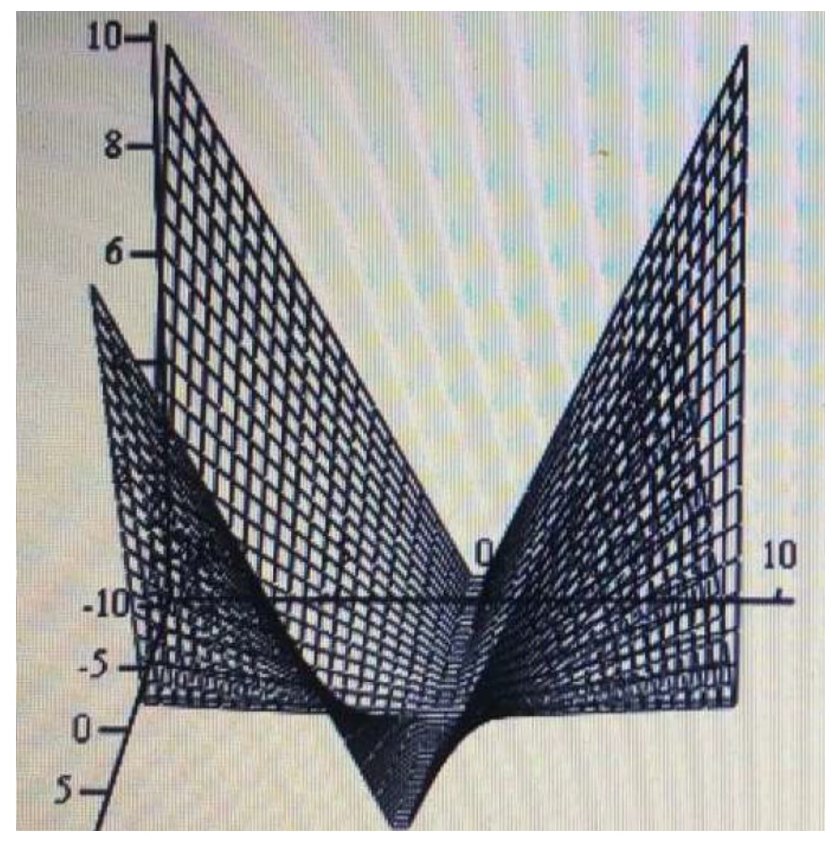
The Lyapunov stability region is depicted in Figure 1, Figure 2 and Figure 3.
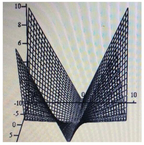
Figure 1.
The region of partial stability for System (15), expressed in the variables , consists of the points above the depicted surface.
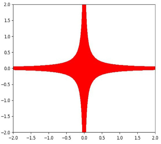
Figure 2.
The region of partial stability for System (15), expressed in the variables with ; as z increases, this region expands.
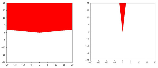
Figure 3.
The region of partial stability for System (15), expressed in the variables , with and , respectively. If , then this region becomes a ray perpendicular to the x-axis; if , then this region will cover the upper semiplane of the -plane. Due to symmetry, the same kind of regions will be in the variables for different y.
This numerical example clearly shows how Lyapunov stability regions, which are obtained using our version of the regularization method, usually look like if several of the system’s parameters are fixed. In particular, these regions are open subsets of the respective partial phase spaces, which means that the property of Lyapunov stability is preserved under small perturbations of the varying parameters. Note that changing the set of varying parameters yields stability regions with similar geometric properties.
The example indicates as well how such an analysis can be performed in other cases considered in the article, including stochastic ones. Indeed, the stability conditions, obtained by the regularization method, are expressed in terms of the system’s parameters. Keeping fixed some of the parameters and aggregating the others into more convenient ones (as we had performed by introducing the variable in the example) would produce inequalities defining stability regions in the corresponding partial phase spaces. We do not include more numerical examples in this article, as this would considerably increase its size.
7. Discussion
This article deals with partial moment stability of hybrid discrete–continuous systems of linear stochastic equations, a complicated problem that apparently has not been studied before. To tackle its theoretical and technical challenges, a modified version of the classical regularization method, based on the choice of an auxiliary equation and the theory of non-negative and positive invertible matrices, has been suggested and justified.
To be able to apply the regularization techniques, we have offered an alternative description of stochastic partial stability in terms of input-to-state stability, known in control theory, in such a way that different spaces of stochastic processes correspond to different kinds of partial stability.
We have also proposed a formalized algorithm as to how a regularization of a given hybrid system can be performed in practice and how this leads to verifiable, coefficient-based stability conditions. We have concentrated on the case of stability with respect to proper subsets of both continuous-time and discrete-time components, while also outlining a method of analysis for the other cases as well.
We have also demonstrated that our algorithm, being primarily designed for the stochastic case, provides new conditions for the partial stability of linear deterministic hybrid systems.
In the future, we plan to study other classes of hybrid stochastic systems—first of all, nonlinear ones, as our previous publications show that the regularization method has such a potential. In addition, we want to extend our analysis to hybrid equations with unbounded delays, where exponential stability should be replaced by more general kinds of asymptotic stability, as more involved auxiliary systems may be necessary to exploit.
Author Contributions
Conceptualization, R.I.K.; methodology, R.I.K. and A.P.; formal analysis, R.I.K.; investigation, R.I.K. and A.P.; writing—original draft preparation, R.I.K.; writing—review and editing, A.P. All authors have read and agreed to the published version of the manuscript.
Funding
This research received no external funding.
Data Availability Statement
The original contributions presented in the study are included in the article, further inquiries can be directed to the corresponding author.
Acknowledgments
The authors would like to express their appreciation for the anonymous reviewers’ in-depth comments, suggestions and corrections, which have greatly improved the presentation of the results.
Conflicts of Interest
The authors declare no conflicts of interest.
Abbreviations
The following abbreviations are used in this manuscript:
| a.s. | almost surely |
| e. g. | exempli gratia (for example) |
| i. e. | id est (that is) |
Appendix A. Conditions for Other Cases of Partial Stability
Conditions M1–M2 and the definition of System (4) are presented in Section 3 for Case 1 (, ). Cases 2–7 require some adjustments, which directly influence the vector solutions , , and in System (4) and the matrices and (), determining the operators in (4), as well as the matrices , in Propositions 1–3. In Appendix A, we formulate these adjustments explicitly, including Case 1 for the sake of completeness. We found it convenient to summarize Conditions M1–M2 in a tabular form. Note that Table A1 and Table A8 describe Conditions M1–M2, respectively, for Case 1 , , which was analyzed in Section 3, Section 4 and Section 5 in detail.
It is important to remark that all results presented in Section 3, Section 4 and Section 5 remain true, and with the same formulations, for any of the seven cases of partial stability, provided that the following adjustments are made:
If a matrix is not defined in a table, then the corresponding matrices , and the matrices , should be removed from System (4) and Propositions 1–3, respectively. The same rule applies to the vector solutions , , and in System (4).
As before, we consider below partial stability with respect to the first continuous-time variables and the first discrete-time variables , so that , and .

Table A1.
Case 1: , .
Table A1.
Case 1: , .
| Size of | Removed Rows | Removed Columns | |
|---|---|---|---|
| Last | Last | ||
| Last | First and last | ||
| Last | First l and last | ||
| First | First | ||
| First | Last | ||
| First | First and last | ||
| Last | First l and last | ||
| First | First | ||
| Last | — | ||
| First | — |
Table A2.
Case 2: , .
Table A2.
Case 2: , .
| Size of | Removed Rows | Removed Columns | |
|---|---|---|---|
| — | Last | ||
| First l | Last | ||
| — | First l | ||
| — | — |
Table A3.
Case 3: , .
Table A3.
Case 3: , .
| Size of | Removed Rows | Removed Columns | |
|---|---|---|---|
| Last | Last | ||
| Last | First and last | ||
| Last | First l | ||
| First | Last | ||
| First | First and last | ||
| Last | — | ||
| First | — |
Table A4.
Case 4: , .
Table A4.
Case 4: , .
| Size of | Removed Rows | Removed Columns | |
|---|---|---|---|
| — | Last | ||
| — | First l | ||
| — | — |
Table A5.
Case 5: , .
Table A5.
Case 5: , .
| Size of | Removed Rows | Removed Columns | |
|---|---|---|---|
| Last | Last | ||
| Last | First and last | ||
| First | First l | ||
| Last | — | ||
| First | — |
Table A6.
Case 6: , .
Table A6.
Case 6: , .
| Size of | Removed Rows | Removed Columns | |
|---|---|---|---|
| First | — | ||
| First l | Last | ||
| — | First | ||
| — | — |
Table A7.
Case 7: , .
Table A7.
Case 7: , .
| Size of | Removed Rows | Removed Columns | |
|---|---|---|---|
| — | First l | ||
| — | — |
Condition M2. In Table A8, Table A9, Table A10, Table A11, Table A12, Table A13 and Table A14, M is an arbitrary matrix.
Table A8.
Case 1: , .
Table A8.
Case 1: , .
| Size of | Removed Rows | Removed Columns | |
|---|---|---|---|
| Last | Last | ||
| Last | First and last | ||
| Last | First l and last | ||
| Last | First | ||
| First | Last | ||
| First | First and last | ||
| First | First l and last | ||
| First | First | ||
| Last | — | ||
| First | — |
Table A9.
Case 2: , .
Table A9.
Case 2: , .
| Size of | Removed Rows | Removed Columns | |
|---|---|---|---|
| Last | Last | ||
| Last | First l and last | ||
| Last | First | ||
| First | Last | ||
| First | First l and last | ||
| First | First | ||
| Last | — | ||
| First | — |
Table A10.
Case 3: , .
Table A10.
Case 3: , .
| Size of | Removed Rows | Removed Columns | |
|---|---|---|---|
| — | Last | ||
| — | First and last | ||
| — | First l | ||
| — | — |
Table A11.
Case 4: , .
Table A11.
Case 4: , .
| Size of | Removed Rows | Removed Columns | |
|---|---|---|---|
| — | Last | ||
| — | First l | ||
| — | — |
Table A12.
Case 5: , .
Table A12.
Case 5: , .
| Size of | Removed Rows | Removed Columns | |
|---|---|---|---|
| — | Last | ||
| — | First and last | ||
| — | First l | ||
| — | — |
Table A13.
Case 6: , .
Table A13.
Case 6: , .
| Size of | Removed Rows | Removed Columns | |
|---|---|---|---|
| Last | Last | ||
| Last | First l and last | ||
| Last | First | ||
| First | Last | ||
| First | First l and last | ||
| First | First | ||
| Last | — | ||
| First | — |
Table A14.
Case 7: , .
Table A14.
Case 7: , .
| Size of | Removed Rows | Removed Columns | |
|---|---|---|---|
| — | Last | ||
| — | First l | ||
| — | — |
The vector solutions , , and included in System (4) and defined in Section 3 for Case 1 (, ) as
should be adjusted to the other cases as follows:
- Case 2: , .
- Case 3: , .
- Case 4: , .
- Case 5: , .
- Case 6: , .
- Case 7: , .
References
- Fazel, R.; Shafei, A.M.; Nekoo, S.R. A new method for finding the proper initial conditions in passive locomotion of bipedal robotic systems. Comm. Nonlin. Sci. Num. Sim. 2024, 130, 107693. [Google Scholar] [CrossRef]
- Borquez, J.; Peng, S.; Chen, Y.; Nguyen, Q.; Bansal, S. Hamilton-Jacobi reachability analysis for hybrid systems with controlled and forced transitions. Robotics 1923, 19, 13. [Google Scholar]
- Schupp, S.; Leofante, F.; Behr, L.; Ábrahám, E.; Taccella, A. Robot swarms as hybrid systems: Modelling and verification. In Symbolic-Numeric Methods for Reasoning About CPS and IoT; Remke, A., Tran, D.H., Eds.; EPTCS 361: Munich, Germany, 2022; pp. 61–77. [Google Scholar]
- Zahedi, A.; Shafei, A.M.; Shamsi, M. Application of hybrid robotic systems in crop harvesting: Kinematic and dynamic analysis. Comp. Electr. Agric. 2023, 209, 107724. [Google Scholar] [CrossRef]
- Kong, N.J.; Payne, J.; Council, G.; Johnson, A.M. The salted kalman filter: Kalman filtering on hybrid dynamical systems. Automatica 2021, 131, 109752. [Google Scholar] [CrossRef]
- Sansana, J.; Joswiak, M.N.; Castillo, I.; Wang, Z.; Rendall, R.; Chiang, L.H.; Reis, M.S. Recent trends on hybrid modeling for Industry 4.0. Comp. Chem. Engin. 2021, 151, 107365. [Google Scholar] [CrossRef]
- Hybrid Energy System Models; Berrada, A., El Mrabet, R., Eds.; Elsevier Academic Press: London, UK, 2021; 371p. [Google Scholar]
- Wu, H.; Huang, Y.; Yin, Z.P. Flexible hybrid electronics: Enabling integration techniques and applications. Sci. China Techn. Sci. 2022, 65, 1–12. [Google Scholar] [CrossRef]
- Heuer, J.; Krenz-Baath, R.; Obermaisser, R. Human-heart-model for hardware-in-the-loop testing of pacemakers. Comp. Biol. Med. 2024, 180, 108966. [Google Scholar] [CrossRef]
- Baldari, L.; Boni, L.; Cassinotti, E. Hybrid robotic systems. Surgery 2024, 176, 1538–1541. [Google Scholar] [CrossRef]
- Coy, S.; Czumaj, A.; Scheideler, C.; Schneider, P.; Werthmann, J. Routing schemes for hybrid communication networks. Theor. Comp. Sci. 2024, 985, 114352. [Google Scholar] [CrossRef]
- Liberzon, D. Switching in Systems and Control; Springer Science & Business Media: Berlin, Germany, 2003; 233p. [Google Scholar]
- Lin, H.; Antsaklis, P.J. Stability and stabilizability of switched linear systems: A survey of recent results. IEEE Trans. Automat. Contr. 2009, 54, 308–322. [Google Scholar] [CrossRef]
- Liberzon, D.; Zharnitsky, V. Almost Lyapunov functions for nonlinear systems. Automatica 2020, 113, 108758. [Google Scholar]
- Teel, A.R.; Subbaramana, A.; Sferlazza, A. Stability analysis for stochastic hybrid systems: A survey. Automatica 2014, 50, 2435–2456. [Google Scholar] [CrossRef]
- Schlotterbeck, C.; Gallegos, J.A.; Teel, A.R.; Núñez, F. Stability guarantees for a class of networked control systems subject to stochastic delays. IEEE Transact. Autom. Contr. 2024, 69, 8884–8891. [Google Scholar] [CrossRef]
- Mao, X.; Yin, G.G.; Yuan, C. Stabilization and destabilization of hybrid systems of stochastic differential equations. Automatica 2007, 43, 264–273. [Google Scholar] [CrossRef]
- Imzegouan, C. Stability for Markovian switching stochastic neural networks with infinite delay driven by Lévy noise. Int. J. Dyn. Contr. 2019, 7, 547–556. [Google Scholar] [CrossRef]
- Liu, D.; Wang, Z.; Zhang, Z.; Liu, J. Partial stabilization of stochastic hybrid neural networks driven by Lévy noise. Sys. Sc. Contr. Eng. 2020, 8, 413–421. [Google Scholar] [CrossRef]
- Vorotnikov, V.I. Partial Stability and Control; Birkhäuser: Basel, Switzerland, 1998; 433p. [Google Scholar]
- Amorim, P.; Casteras, J.-B.; Dias, J.P. On the existence and partial stability of standing waves for a nematic liquid crystal director field equation. arXiv 2023, arXiv:2312.09035v1. [Google Scholar] [CrossRef]
- Caraballo, T.; Ezzine, V.; Hammami, M.A. Partial stability analysis of stochastic differential equations with a general decay rate. J. Engr. Math. 2021, 130, 17. [Google Scholar] [CrossRef]
- Mchiri, L.; Caraballo, T.; Rhaima, M. Partial asymptotic stability of neutral pantograph stochastic differential equations with Markovian switching. Adv. Cont. Discr. Mod. 2022, 18, 15. [Google Scholar] [CrossRef]
- Vorotnikov, V.I.; Martyshenko, Y.G. Partial stability in probability of nonlinear stochastic discrete-time systems with delay. Autom. Remote Contr. 2024, 8, 20–35. [Google Scholar]
- Kadiev, R.I. Sufficient conditions of partial stability of linear stochastic equations with aftereffect. Russ. Math. J. Izv. Vuz. 2000, 6, 75–90. [Google Scholar]
- Garg, K.; Panagou, D. Finite-time stability of hybrid systems with unstable modes. Front. Control Eng. Sec. Nonlin. Control. 2021, 2, 707729. [Google Scholar] [CrossRef]
- Azvelev, N.V.; Simonov, P.M. Stability of Differential Equations with Aftereffect; Taylor and Francis: London, UK, 2002. [Google Scholar]
- Ponosov, A.; Kadiev, R.I. Inverse-positive matrices and stability properties of linear stochastic difference equations with aftereffect. Mathematics 2024, 12, 2710. [Google Scholar] [CrossRef]
- Kadiev, R.I.; Ponosov, A. Stability analysis of solutions of continuous–discrete stochastic systems with aftereffect by a regularization method. Diff. Eqs. 2022, 58, 433–454. [Google Scholar] [CrossRef]
- Sontag, E.D. Input-to-State Stability. In Encyclopedia of Systems and Control; Baillieul, J., Samad, T., Eds.; Springer: Cham, Switzerland, 2001; 9p. [Google Scholar]
- Liptser, R.S.; Shirjaev, A.N. Theory of Martingales; Kluwer: Dordrecht, The Netherlands, 1989. [Google Scholar]


Disclaimer/Publisher’s Note: The statements, opinions and data contained in all publications are solely those of the individual author(s) and contributor(s) and not of MDPI and/or the editor(s). MDPI and/or the editor(s) disclaim responsibility for any injury to people or property resulting from any ideas, methods, instructions or products referred to in the content. |
© 2025 by the authors. Licensee MDPI, Basel, Switzerland. This article is an open access article distributed under the terms and conditions of the Creative Commons Attribution (CC BY) license (https://creativecommons.org/licenses/by/4.0/).