Safe Path Planning Method Based on Collision Prediction for Robotic Roadheader in Narrow Tunnels

Abstract

Safe path planning is essential for the autonomous operation of robotic roadheader in narrow underground tunnels, where limited perception and the robot’s geometric constraints present significant challenges. Traditional path planning methods often fail to address these issues. This paper proposes a collision prediction-integrated path planning method tailored for robotic roadheader in confined environments. The method comprises two components: collision prediction and path planning. A collision prediction model based on artificial potential fields is developed, considering the non-convex shape of the roadheader and enhancing scalability. By utilizing tunnel design information, a composite potential field model is created for both obstacles and the roadheader, enabling real-time collision forecasting. The A* algorithm is modified to incorporate the robot’s motion constraints, using a segmented weighted heuristic function based on collision predictions. Path smoothness is achieved through Bézier curve smoothing. Experimental results in both obstacle-free and obstacle-laden scenarios show that the proposed method outperforms traditional approaches in terms of computational efficiency, path length, and smoothness, ensuring safe, efficient navigation in narrow tunnels.

1. Introduction

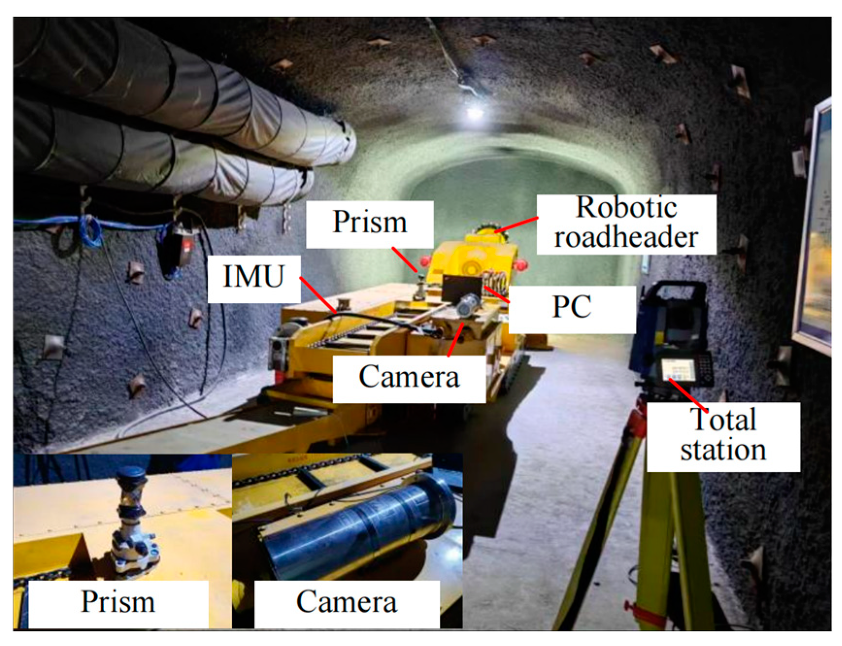
Safe path planning is essential for enabling autonomous navigation of robotic roadheader, playing a critical role in enhancing automation and operational efficiency in coal mining [1]. Robotic roadheaders are commonly used in tunneling operations in complex conditions, as shown in Figure 1. These machines consist of a mobile tracked chassis and a cutting arm, with position control managed by the chassis and cutting performed by the swinging arm. During operation, they face challenging environments with low lighting and high dust, which hinder real-time perception. The narrow tunnel spaces further limit automation and intelligence development. Consequently, path planning in such confined areas with limited perception is particularly difficult [2]. Ensuring safe path planning in narrow tunnels is a critical challenge in current robotic roadheader autonomous control research.

Current research on path planning and control for robotic roadheader mainly focuses on pose adjustment and deviation correction, with an emphasis on localized motion control. Fang et al. developed a dynamic attitude compensation method for real-time control [3], which offers effective adjustment but may be limited by its focus on localized motion neglecting global path planning challenges. Li et al. proposed a fuzzy neural network PID control method for attitude adjustment to address trajectory deviations [4], offering adaptability but potentially suffering from high computational cost and the need for extensive parameter tuning. Ji et al. proposed a path rectification and tracking algorithm using particle swarm optimization, considering road conditions and roadheader performance [5]. While it efficiently explores search spaces, it may struggle with convergence in dynamic environments. Zhang et al. designed a reduced-order active disturbance rejection controller to compensate for pose deviations [6], which rejects disturbances but might struggle with complex multi-objective tasks in constrained tunnel environments. Despite these advances, most robotic roadheader rely on localized motion control, which is inadequate for autonomous operation, especially in narrow tunnel environments. Our team explored relocation path planning for robotic roadheader using reinforcement learning, demonstrating effectiveness in confined environments [7]. However, this method requires a pre-established environment model for training and entails high computational complexity [8]. In coal mining, research on autonomous control of robotic roadheader has mainly focused on cross-sectional cutting, with less emphasis on body motion control. Effective motion planning must consider the robot’s dimensions, tunnel environment, and motion constraints.

Recent studies have combined path planning algorithms with environmental perception to develop local dynamic path planning methods [9,10]. Chou et al. employed intelligent perception technologies to update optimal paths [11], providing a promising approach for path adaptation, though potentially limited by perception system reliability in challenging environments. Li et al. [12] formulated path planning as an optimal control problem solved using adaptive dynamic programming and artificial potential fields, which provides a robust theoretical framework, though its computational complexity may limit real-time application. While these methods perform well in indoor environments, they face robustness challenges in low-light, harsh mining conditions, where vision-based and Lidar-based perception systems often struggle [13], revealing a significant limitation in practical mining applications. Cui et al. [14] presents a multi-sensor fusion positioning system using EKF and UKF to accurate positioning in GPS-denied underground coal mines, though its robustness may be affected by varying conditions and vibrations. Ren et al. [15] proposed a graph SLAM optimization method using GICP 3D point cloud registration with roadway constraints to enhance localization in underground mining environments, though its effectiveness may be hindered by noise and occlusion in dynamic conditions. Thus, path planning for robotic roadheader in limited-perception environments can be defined as global path planning with spatial constraints in narrow tunnels. Traditional methods often rely on idealized models, such as grid maps or feature maps, often neglecting the robot’s geometric and environmental constraints [16,17], leading to suboptimal paths that require real-time adjustments or collision detection, increasing system complexity. Narrow tunnels present unique challenges due to the non-convex geometry and complex motion constraints, making traditional methods inadequate.

In this context, collision prediction becomes critical for ensuring safe robotic operation. By tracking the position of robots and obstacles in real time, collision prediction enables dynamic path adjustments to avoid collisions. Herrmann et al. introduced deep collision probability fields for autonomous driving, laying the foundation for path planning [18], though its applicability in mining environments with irregular and constrained spaces, may require further adaptation. Ji et al. proposed a virtual danger potential field for collision-free path planning [19], offering an innovative solution but may be computationally expensive and less effective in dynamic environments. Wang et al. [20] designed a motion planning method to mitigate collisions in emergencies, which is effective in critical situations but may lack a proactive, continuous solution for path planning. Chen et al. developed a path tracking and stability control strategy for extreme driving conditions [21], providing robust performance in difficult conditions, though its reliance on specific driving scenarios might limit its broader applicability. Path smoothness is another crucial aspect, particularly in narrow tunnels where smooth paths directly influence motion efficiency and stability. Techniques such as Bézier curves have been widely applied for path smoothing [22,23], offering a useful method for generating smooth trajectories but often requiring additional computational resources in real-time applications. Bi et al. [24] proposed a dual-Bézier transition method for simultaneously smoothing translational and rotational tool paths, improving robot stability, which provides an effective solution but may be complex to implement in systems with strict real-time performance requirements.

In summary, while existing research has made progress in path planning, collision prediction, and path smoothing, significant gaps remain. Most methods focus on local dynamic path planning, neglecting the safety of global static planning, especially under complex environmental constraints and with consideration of robot geometry. This study addresses these challenges by proposing a collision prediction-integrated path planning method for robotic roadheader. The method establishes a collision prediction model using artificial potential fields and calculates collision probabilities based on robot pose. It improves the A* algorithm to generate safe paths and offers a new perspective for solving path planning problems in narrow tunnels. The main contributions of this study are as follows:

(1)

A collision prediction-integrated path planning method is proposed to address the safety challenges of robotic roadheader in narrow coal mine tunnels, providing a foundation for achieving autonomous control.

(2)

A collision prediction model based on artificial potential fields is developed. Using prior tunnel design information, the model constructs a mathematical tunnel representation and composite potential fields for tunnels, obstacles, and the robot, enabling real-time collision prediction.

(3)

An improved A* method for robotic roadheader is presented. By incorporating collision prediction factors, designing a segmented weighted heuristic function, optimizing search neighborhoods, and applying Bézier curve smoothing, the method enhances path planning efficiency, safety, and smoothness.

The rest of this paper is organized as follows. Section 2 describes safe path planning problem for robotic roadheader in narrow tunnels. Section 3 depicts the method of safe path planning based on collision prediction. Section 4 presents the experimental verification and analysis of related methods. Section 5 provides the discussion of the results. Finally, the conclusion and future work are presented in Section 6.

2. Problem Statement

The robotic roadheader consists of two subsystems: the mobile chassis and the cutting arm. Its operation involves two main tasks: moving and cutting. The mobile chassis moves the robot to the target position, while the cutting arm handles sectional cutting. This study focuses on the safe path planning of the mobile chassis, excluding the cutting task during movement. The starting point $D_1$ is typically positioned on one side of the roadway to allow space for transportation and row formation. Left and right cutting positions are designed, multiple cuts may be required when the cutting space is smaller than the target. as multiple cuts may be required when the cutting space is smaller than the target. After the cut is complete, it is necessary to stop at $D_2$, which advances a target section depth relative to $D_1$. As illustrated in Figure 2, the robotic roadheader operates within a confined tunnel, requiring several movements to complete the cutting plan.

Specifically, the motion of robotic roadheader follows a cyclic cutting process, as each cut is time-consuming and requires safety support. In each cycle, the robot starts from the initial position $D_1$, moves to the first cutting point $O_1$, waits for the cut to finish, moves to $O_2$, and then cuts the remaining target area. Afterward, it returns to the stopping point $D_2$, and the next cycle begins from there. The autonomous operation of the robotic roadheader in narrow tunnels presents two main challenges for safe path planning:

(1)

Limited Environmental Perception: The harsh conditions of coal mines, including low lighting and high dust levels, pose significant challenges for environmental perception systems, limiting awareness of the surroundings.

(2)

Constrained Operational Space: In narrow tunnels, spatial limitations restrict the movement and maneuverability of robotic roadheader, unlike in open environments.

In this context, safe path planning for the robotic roadheader can be framed as a local path planning problem, considering the robot’s geometric constraints without real-time environmental perception. The robot’s dimensions, including the operational mechanism size, directly affect the feasibility and safety of the planned path.

The goal of path planning for the robotic roadheader is to find the shortest collision-free path on a known map from a starting point $S$ to a target point $G$. In general, obstacles may exist between $S$ and $G$, but in the narrow tunneling space discussed in this paper, there are no obstacles. The space is semi-enclosed with defined boundaries, so a collision-free path ensures the roadheader avoids collisions with the tunnel boundaries. Given the low likelihood of obstacles, they are considered static in this scenario.

$$P=\left(p_i,{\theta }_i\right)=\left\{(S,0),(p_1,{\theta }_1),\cdots ,(G,0)\right\}$$

(1)

When the robot is at position $p_i$ with a heading angle of ${\theta }_i$, it must avoid colliding with the boundaries and the line connecting to the adjacent position. The first step is to consider the robot’s size, heading, and tunnel constraints in developing a suitable path search method. Collision detection should also be performed during the search to ensure the path remains safe and collision-free.

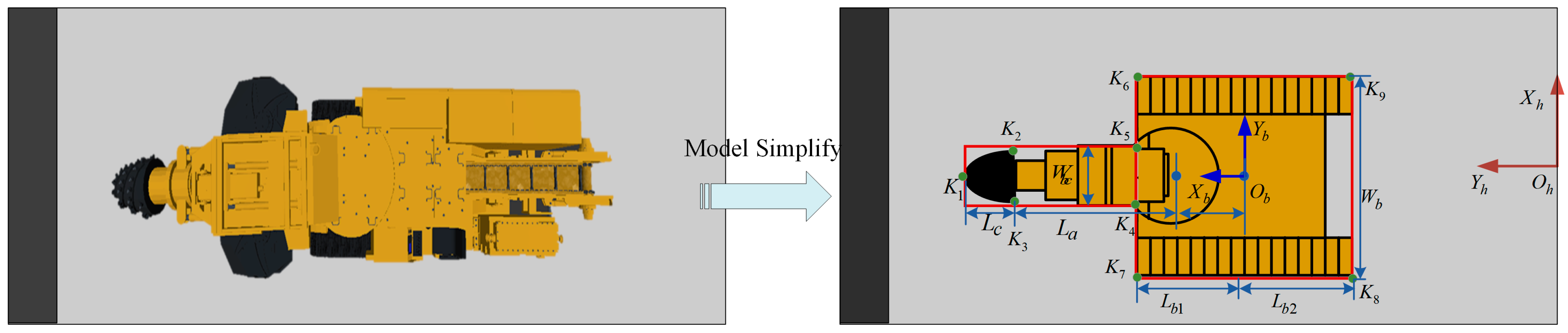
Geometric Constraints. Based on the position and orientation information of the robotic roadheader, combined with its shape and size parameters, the coordinates of key points on the boundary contour of the tunnel boring machine are calculated in real time to form the size constraints of the robot. Figure 3 presents a simplified model of the robotic roadheader.

Each protruding point is identified as a key point $K_i(i=1,2,\dots ,9)$, which will be used for collision calculations during the planning process. Figure 3 also includes the roadway $O_h-X_h{Y}_h$ and body coordinates $O_b-X_b{Y}_b$, along with key dimensional parameters of the robotic roadheader, for use in subsequent simulations and calculations.

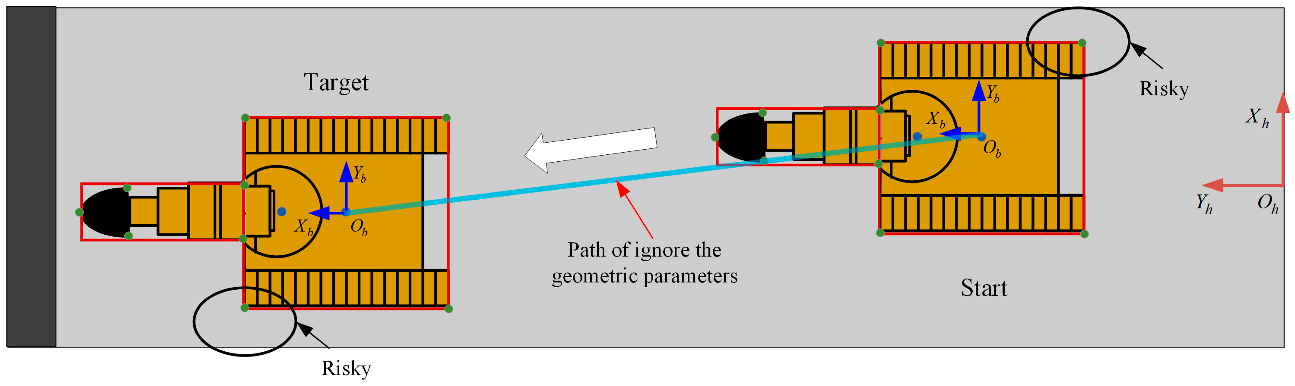
When the robot moves in a narrow tunnel, treating it as a point mass results in a path that is a straight line between the start and target, as shown by the blue segment in Figure 4. Using this as a reference path for control would cause a collision, as illustrated in the figure. Therefore, considering the robot’s geometric parameters is essential in narrow tunnels.

Heading Constraints. The robotic roadheader is a tracked robot. In general, tracked robots can rotate in place and move forward in any direction. However, in this confined scenario, due to the limited space and the coordination with equipment such as the transport plane, the robot’s rotation angle is restricted to a certain limit to avoid danger. That is, $\theta \le {\theta }_{\max }$.

Tunneling Scenario Constraints. The tunnel space is narrow and pre-designed. While minor construction deviations may occur, strict standards ensure these errors remain within a controllable range, allowing accurate modeling of the tunnel boundaries and centerline. The model focuses on the left and right boundaries, as they directly affect the machine’s lateral motion. The vertical direction, with sufficient clearance, is stable and negligible for planning. Thus, the digital model of the tunnel boundaries and centerline is as follows:

$$\left\{\begin{array}{ll}{x}_l=-0.5W_h,\hfill & y_l\in \left[0,L_h\right]\hfill \\ x_r=0.5W_h,\hfill & y_r\in \left[0,L_h\right]\hfill \\ x_{mid}=0,\hfill & y_{mid}\in \left[0,L_h\right]\hfill \end{array}\right.$$

(2)

where $(x_l,y_l)$ and $(x_r,y_r)$ represent the coordinates of the left and right tunnel boundaries, respectively, and $(x_{mid},y_{mid})$ represents the coordinates of the tunnel centerline.

3. Materials and Methods

3.1. Overall Framework

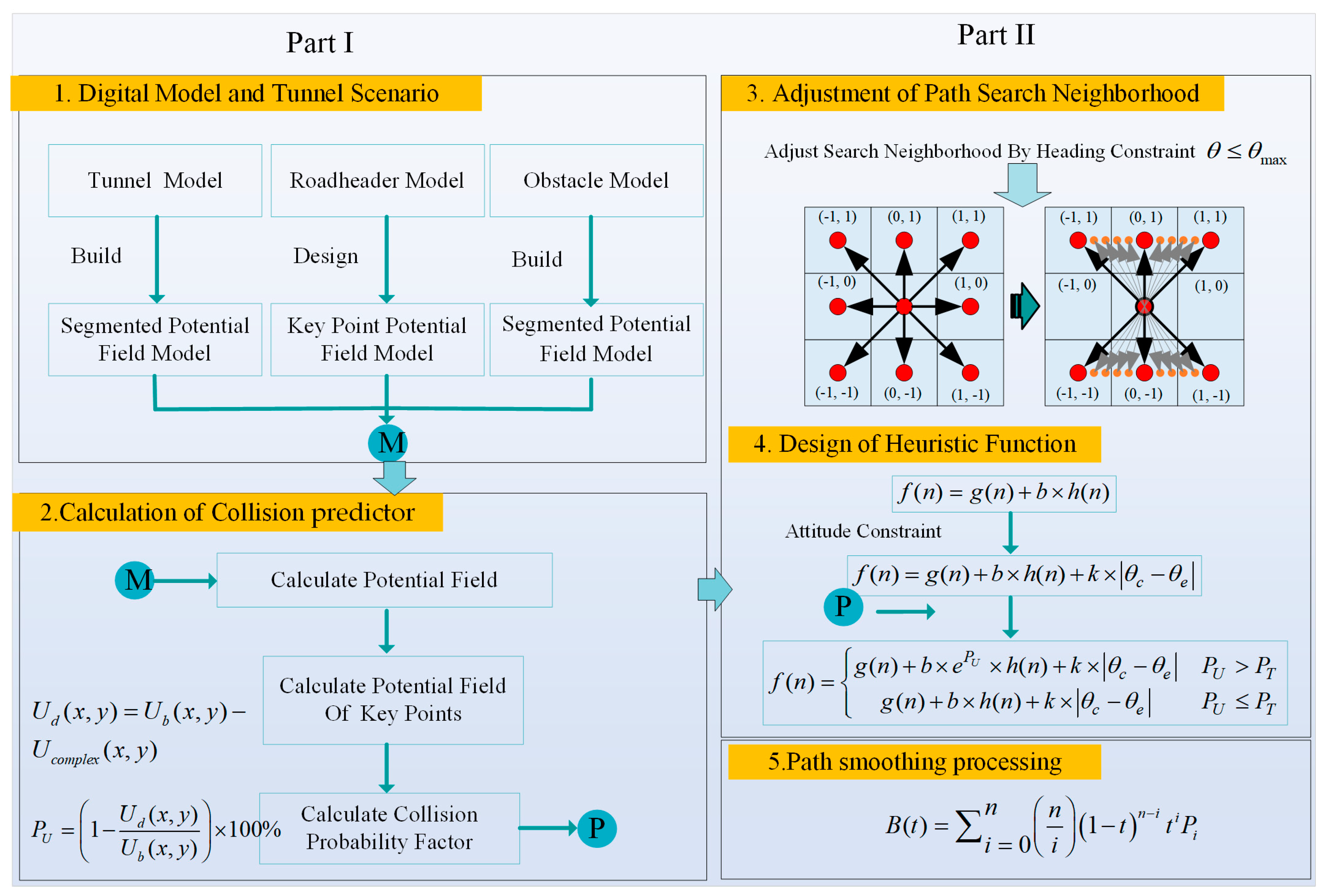
This paper aims to develop a safe path planning method for robotic roadheader in narrow tunnels, enabling autonomous and efficient navigation in challenging underground environments. The approach includes two components: collision prediction and path planning. The overall framework is shown in Figure 5.

Part I of this study uses digital models of the tunnel, roadheader, and obstacles to create a composite artificial potetial field for collision prediction. The roadheader calculates potential differences at key points along its boundary in real time to predict collisions. Given the limited environmental perception in coal mine tunnels, this real-time prediction is essential. We propose a model based on artificial potential fields to handle the roadheader’s non-convex shape and the complex tunnel environment. Using prior tunnel design data, the model constructs a mathematical representation of the tunnel and integrates the potential fields for the robot, obstacles, and tunnel. By tracking the robot’s pose, the model dynamically predicts potential collisions, allowing for timely path adjustments.

In Part II, we adjust the A* heuristic search based on the roadheader’s heading constraints in narrow tunnels for a more accurate trajectory. We then integrate the collision prediction results from Part I into a safety-aware heuristic. To improve efficiency, a distance threshold and a segmented heuristic function are introduced to reduce computational load while maintaining safety. Bézier curve smoothing is applied to the turning points of the path, eliminating sharp corners and enhancing stability.

By combining collision prediction with optimized path planning, this method ensures the roadheader can navigate narrow tunnels safely and efficiently, even in environments with limited perception and static obstacles. The method provides a comprehensive solution for autonomous navigation in complex underground spaces, laying the foundation for future advancements in robotic mining operations.

3.2. Collision Prediction Model Using Artificial Potential Field

We designed artificial potential fields for narrow tunnels, obstacles, and the boundaries of the robot, among others. By integrating these potential fields, a composite potential field is constructed to calculate the real-time variation of the robot boundary potential field. By integrating these potential fields, a composite potential field is constructed to calculate the real-time variation of the robot boundary potential field. Based on these changes, we can evaluate the likelihood of a collision.

3.2.1. Design of Tunnel Potential Field

According to different risk levels, a piecewise function is established to represent the tunnel space constraint potential field [25]. It is assumed that the high-risk area is within $t$ m from the side wall of the tunnel, and the other locations are low risk areas. A rapidly changing exponential function is used to establish the spatial constraint potential field of the tunnel in the high-risk area. In the low-risk area, trigonometric functions are used to establish the spatial constraint potential field of the tunnel.

$$U_{road}=\left\{\begin{array}{ll}{\eta }_{road1}[e^{\left|2(x-t)\right|}+\psi ]\hfill & ,0\le x\le t\hfill \\ {\eta }_{road2}\left[\sin ({\psi }_{1}x+{\psi }_2)\pi +1\right]\hfill & ,t\le x\le W_h-t\hfill \\ {\eta }_{road1}[e^{\left|2(x-(W_h-t))\right|}+\psi ]\hfill & ,W_h-t\le x\le W\hfill \end{array}\right.$$

(3)

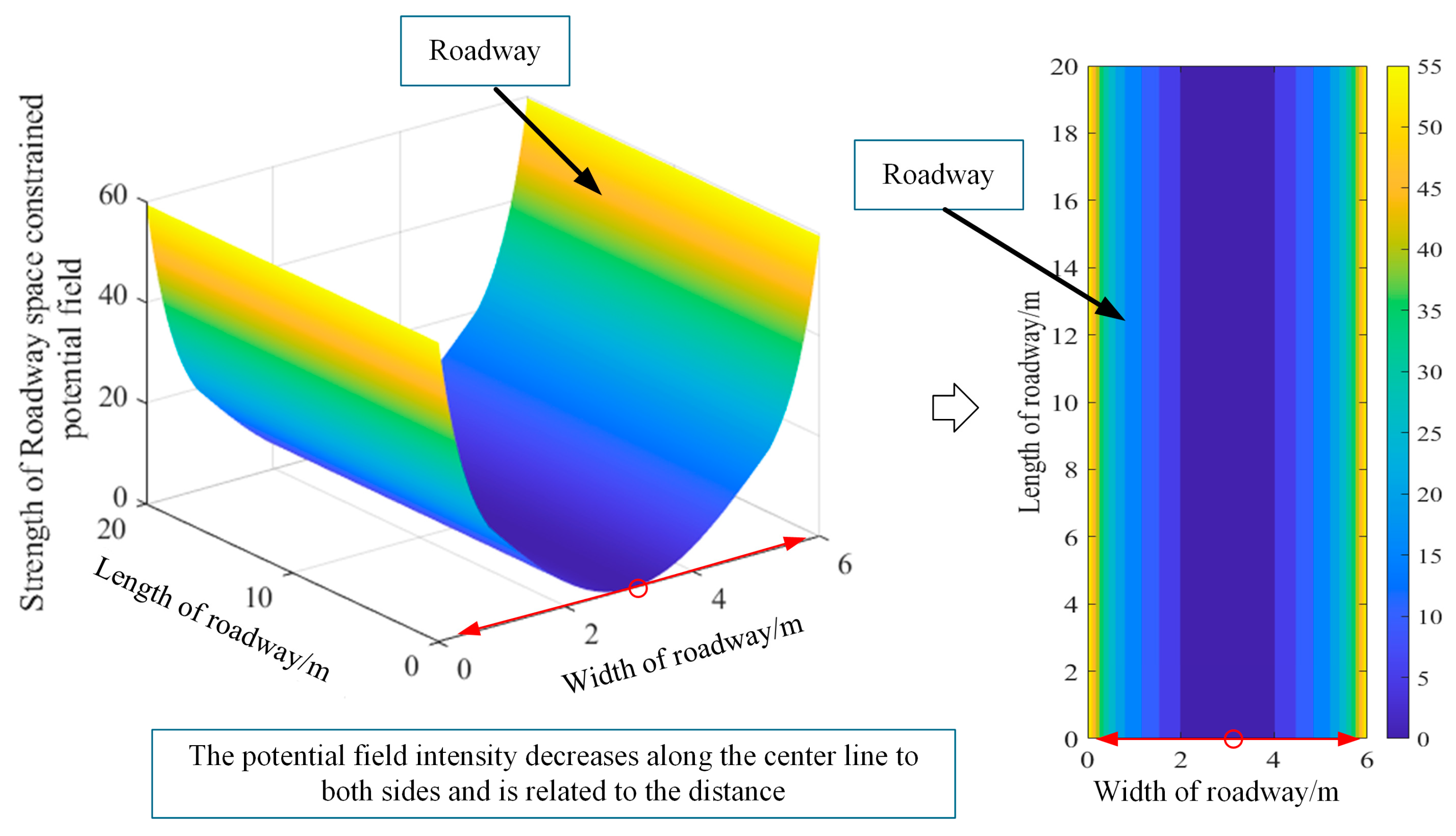
where ${\eta }_{road1}$ is the repulsive potential field coefficient of the high-risk region; ${\eta }_{road2}$ is the repulsive potential field strength coefficient in the low-risk region. Define ${\eta }_{road1}=10$, ${\eta }_{road2}=20$, $W_h=6$, $\psi =1$, ${\psi }_1=5/22$ and ${\psi }_2=9/11$, and establish the spatial constraint potential field diagram of the tunnel according to Equation (3), as shown in Figure 6.

According to Equation (3) and Figure 6, the potential field intensity is large and changes rapidly on both sides of the approaching tunnel. The potential field intensity in the area near the middle of the tunnel is small, and the change trend is relatively slow. The intensity of the potential field at the center line of the tunnel is 0.

3.2.2. Design of Obstacle Potential Field

Obstacles in narrow underground environments are often irregular in shape. For simplicity, this paper models them as circular protrusions, though the approach can be extended to other shapes. Inside the obstacle, a uniform potential field $U_{in}$ is assigned a constant value. Beyond the obstacle’s maximum effective range, the potential field rapidly diminishes to zero. Between the boundary and the maximum range, the potential field value increases as the distance decreases, which is modeled using an exponential function to ensure that the field strength grows closer to the obstacle and decays with distance.

Furthermore, a smoothing factor, denoted as $s$, is introduced to ensure a smoother transition in the potential field. The piecewise potential field distribution function for obstacles can be expressed as:

$$U_r=\left\{\begin{array}{ll}{U}_{in},\hfill & r\le R\hfill \\ U_{in}\cdot \exp \left(-s\cdot {(\frac{r-R}{R_{de}})}^2\right),\hfill & R<r\le R+R_{de}\hfill \\ 0,\hfill & r>R+R_{de}\hfill \end{array}\right.$$

(4)

In the equation, $r$ represents the distance from the current point to the center of the obstacle, $s$ denotes the smoothing factor, $R$ signifies the radius of the obstacle, and $R+R_{de}$ indicates the maximum effective range of the potential field of obstacles.

The design follows the principle that the potential field strength increases as the distance to the obstacle decreases. While the model uses circular approximations for simplicity, the approach can be adapted to irregularly shaped obstacles by adjusting the potential field function to reflect the impact of distance, maintaining similar exponential behavior. Figure 7 shows the artificial potential field distribution of obstacles. The potential is at a maximum inside the obstacle and decreases with distance from its boundary. Once the distance exceeds a certain threshold, the potential becomes zero.

3.2.3. Design of Potential Field for Robotic Roadheader

The coordinate origin is established at the center of the robotic roadheader, with the x-axis pointing forward and the y-axis pointing laterally. The coordinates of key points $K_1~K_9$ are illustrated in Figure 3. By calculating the coordinates $P_k$ of these key points in the current position, the center coordinates ${\left[\begin{array}{cc}{x}_0& y_0\end{array}\right]}^T$ and heading angle $\theta$ of the robotic roadheader can be obtained.

$$P_k=\left[\begin{array}{l}{x}_i\\ y_i\end{array}\right]=\left[\begin{array}{cc}\cos \theta & \sin \theta \\ -\sin \theta & \cos \theta \end{array}\right]\left[\begin{array}{l}{x}_{b_i}\\ y_{b_i}\end{array}\right]+\left[\begin{array}{l}{x}_0\\ y_0\end{array}\right],i=1,2\dots 9.$$

(5)

where $\left[\begin{array}{cc}{x}_{b_i}& y_{b_i}\end{array}\right]$ represents the coordinates of the key points of the roadheader boundary in the body coordinate system, which can be calculated by the fuselage size. Utilizing the aforementioned methodology, the coordinates of the boundary points of the robotic roadheader can be computed in real time based on its current pose and position. By acquiring the potential difference at these points, one can ascertain whether a collision will occur at the current path point, thereby enabling early assessment of the path. Between the key points defining the external contour, a linear interpolation approach is employed to derive the precise coordinates of the entire boundary contour. To guarantee a thorough evaluation of the robotic collision potential energy, a fixed potential field value $U_f$ is assigned to each coordinate on the outer contour, and $U_f=55$.

$$U_b(x_i,y_i)=U_f,i=1,2\dots 9.$$

(6)

3.2.4. Collision Predictor

The composite potential field distribution of obstacles in a narrow tunnel can be represented as a combination of two potential fields. Assuming there is a point $(x,y)$ within the passage, the original potential field value at this point is denoted as $U_{road}$, and the potential field value of the obstacle is denoted as $U_r$. The superposition method can be expressed as:

$$U_{complex}(x,y)=\max (U_{road}(x,y),U_r(x,y))$$

(7)

Therefore, based on the composite artificial potential field described in the previous section, the potential difference at any point within the boundary of the robotic roadheader in the composite artificial potential field is designed as follows:

$$U_d(x,y)=U_b(x,y)-U_{complex}(x,y)$$

(8)

Based on the known composite potential field distribution of tunnel and obstacles, the potential field difference $U_d$ at the boundary of the lane where the robot is located can be accurately and rapidly calculated. Definition of the collision predictor $P_U$:

$$P_U=\left(1-{\displaystyle \frac{U_d(x,y)}{U_b(x,y)}}\right)\times 100\%$$

(9)

Based on practical considerations, we set a threshold parameter $T$ for collision warning. When the collision predictor $P_U>T$, it indicates that the robot is about to collide with other objects and requires timely adjustments.

To assess the collision probability for the entire outer contour of the robot, we select the maximum value $\max (P_U)$ as the criterion for determining whether a collision will occur. In this process, the composite potential field distribution of the narrow tunnel and obstacles is crucial prior data.

To better illustrate the processing steps of the proposed method, we provide pseudocode for calculating the collision prediction factors (see Algorithm 1).

Algorithm 1: Calculate collision predictor

1: function CollisionPrediction(X_lane, Y_lane, U_lane, digital_bmt) 2: input: X_lane, Y_lane, U_lane: Grid coordinates and lane potential field; digital_bmt: Robot’s coordinates 3: output: Pu_max: Maximum collision potential; point_oc: Corresponding point where the maximum collision po tential occurs. 4:  // Initialize robot’s coordinates 5:  bx, by = digital_bmt(1, :), digital_bmt(2, :) 6:  // Get interpolated points and robot’s bottom trajectory 7:  [interp_points, interpolated_Z_all] = Robot_btm(bx, by)//Interpolate the robot boundary key points 8:  nearest_indices = zeros(size(interp_points, 1), 2) 9:  U_lane_with_obstacle = U_lane 10:   PU = [] 11:   //For each interpolated point 12:   for each i in 1 to size(interp_points, 1) 13:    distances_squared = (X_lane(:) − interp_points(i, 1))2 + (Y_lane(:) − interp_points(i, 2))2 14:    min_index = min(distances_squared) 15:    [row_idx, col_idx] = ind2sub(size(X_lane), min_index) 16:    nearest_indices(i, :) = [row_idx, col_idx] 17:    U_lane_with_obstacle(row_idx, col_idx) = interpolated_Z_all(i) − U_lane(row_idx, col_idx) 18:   end for 19:   //Calculate collision potential for each nearest point 20:   for each j in 1 to size(nearest_indices, 1) 21:    U_lane_with_obstacle2 = U_lane(nearest_indices(j, 1), nearest_indices(j, 2)) 22:    PUt = (interpolated_Z_all(j) − U_lane_with_obstacle2)/interpolated_Z_all(j) 23:    PU(j) = 1 − PUt 24:   end for 25:   // Find the maximum collision potential and the corresponding point 26:   Pu_max, max_index = max(PU) 27:   point_oc = nearest_indices(max_index) 28:   return Pu_max, point_oc 29: end function

3.3. Improved A* Path Planning Method Integrating Collision Prediction

3.3.1. Adjusting the Search Neighborhood

Considering the scenario where robots may navigate in narrow tunnels while transporting additional support equipment, the presence of maximum steering constraints poses challenges to the direct application of the A* search method. Therefore, an improved search methodology is necessary to balance computational efficiency and operational feasibility. In practice, the robotic roadheader moves at a very slow speed within a confined working space, typically covering distances of around 10 m. Additionally, coal mine tunnel construction typically requires boundary errors to be controlled within 10 cm, making precise body control crucial for accurate excavation.

In the left subplot of Figure 8, the search grid has a resolution of 1 m × 1 m, which is appropriate for typical tunnel widths of approximately 5 m. Directly applying higher path precision could jeopardize safety and computational feasibility. Using a lower-resolution search grid would significantly increase computation time, thus reducing operational efficiency. Therefore, we further subdivided the 1 m × 1 m search grid to improve path planning accuracy while managing computation time, as demonstrated in the right subplot of Figure 8.

Assuming that the maximum swing angle of the robotic roadheader is $\theta$, and as the robot advances one unit distance along the y-axis, the maximum penetration distance in the x-axis is denoted as 1. By discretizing the x-axis, a new search neighborhood L can be obtained. Simultaneously, by connecting the discrete candidate path points with the base point, a new path is formed. At the juncture, the path is oriented. Assuming the coordinates of the discrete path point at this location are $(x_i,y_i)$ and the base point coordinates are $(0,0)$, the travel direction can be calculated as ${\theta }_i={\tan }^{-1}(x_i,y_i)(i=1,2,\dots )$. Note that this direction has a sign, as illustrated in Figure 8.

The A* search neighborhood is depicted in the left-hand side of Figure 6, with search steps of 1 in both the x-axis and y-axis. The original neighborhood points in the x-axis are evenly divided into five equal segments, as shown in the right-hand side of Figure 6.

3.3.2. Design of the Heuristic Function

The A* search algorithm is a widely used pathfinding and graph traversal algorithm known for its efficiency and accuracy. It combines the strengths of Dijkstra’s algorithm and Greedy Best-First Search by using a cost function:

$$f(n)=g(n)+h(n)$$

(10)

where $g(n)$ represents the cost to reach the current node $n$ from the start node, and $h(n)$ is a heuristic estimate of the cost from $n$ to the goal. The algorithm prioritizes nodes with the lowest $f(n)$, ensuring that it explores the most promising paths first. A* guarantees the shortest path if the heuristic $h(n)$ is admissible and consistent. It is commonly applied in robotics, video games, and navigation systems.

Despite its advantages, the traditional A* algorithm has limitations when applied to narrow underground environments, particularly for robotic roadheader. The method does not account for the posture or orientation of the robot, which can significantly affect the feasibility and safety of the planned path in constrained spaces. To address these limitations, we propose an enhanced weighted A* algorithm that incorporates roadheader posture and collision prediction into the heuristic function.

To enhance search efficiency, a weighted A* algorithm modifies the heuristic function by introducing a weight $b$, which adjusts the influence of the heuristic estimate on the search process. The heuristic function for the weighted A* algorithm is defined as:

$$f(n)=g(n)+b\times h(n)$$

(11)

Here, $b$ is a weight factor that balances exploration and exploitation. A higher $b$ value prioritizes heuristic estimates, potentially increasing search speed but at the cost of accuracy. During the search process of the A* algorithm, the node with the smallest $f(n)$ value is selected from the priority queue as the next node to be traversed. However, this process does not consider the posture of the roadheader. To address this limitation, the posture is incorporated into the heuristic function and simultaneously subjected to weighting.

$$f(n)=g(n)+b\times h(n)+k\times \left|{\theta }_c-{\theta }_e\right|$$

(12)

Specifically, the parameter k serves as a weighting coefficient that determines the impact of posture on the heuristic. To further improve safety, we introduce a collision predictor $P_U$ into the heuristic function. Additionally, to enhance responsiveness and improve performance in narrow tunnel environments, an exponential function $e^{P_U}$ is adopted to further ensure safety. The predictor assesses the proximity of the roadheader to obstacles and dynamically adjusts the heuristic value to prioritize safer paths. The enhanced heuristic function is defined as:

$$f(n)=\left\{\begin{array}{cc}g(n)+b\times e^{P_U}\times h(n)+k\times \left|{\theta }_c-{\theta }_e\right|& P_U>P_T\\ g(n)+b\times h(n)+k\times \left|{\theta }_c-{\theta }_e\right|& P_U\le P_T\end{array}\right.$$

(13)

Given a segmented threshold $P_T$, the heuristic function incorporating the collision factor is utilized to dynamically adjust the heuristic process. To ensure flexibility, we introduce a segmented threshold $P_T$ for the collision predictor. When the distance to an obstacle falls below $P_T$, the collision factor is activated, dynamically adjusting the heuristic to emphasize obstacle avoidance. The segmentation allows the algorithm to balance efficiency and safety across different regions of the environment.

To better explain the proposed the proposed improved A* path planning method integrating collision prediction, we provide the pseudocode for its implementation (see Algorithm 2).

Algorithm 2: Improved A* method based on collision-prediction

1: function Evaluation(n) 2: if Pu > $P_T$ Then 3:   f(n) = g(n) + b ×$e^{P_U}$ × h(n) + k × $\left|{\theta }_c-{\theta }_e\right|$ 4: else 5:   f(n) =g(n) + b × h(n) + k × $\left|{\theta }_c-{\theta }_e\right|$ 6: end if 7: return f(n) 8: end function 9: function updateState (n, n’) 10: c(n, n’) = abs(n. x − n’. y) + abs(n. y − n’. y) //Calculate the cost of going from n to n’ 11: collision_risk = CollisionPrediction() //Perform collision prediction for n and n’ 12: if n’ is an obstacle OR n’ $\in$ CLOSED OR collision_risk > threshold then 13:    ignore this n’  //Ignore nodes with high collision risk 14: else 15:    if n’ $\in$ OPEN then 16:    // Already in the open list, check if there is a better path 17:     if g(n’) > g(n) + c(n, n’) then 18:       parent(n’) = n 19:       g(n’) = g(n) + c(n, n’)  //The cost of updating n’ 20:       Evaluation(n’)  / Reevaluate node n’ 21:     else 22:       ignore this n’ 23:     end if 24:    else 25:      // Insert node n’ into the open list 26:      OPEN. Insert(n’, Evaluation(n’)) 27:      parent(n’) = n 28:      g(n’) = g(n) + c(n, n’) 29:    end if 30: end if 31: end function 32: function Main() 33: g(nstart) = 0 34: OPEN = $\varphi$ 35: CLOSED = $\varphi$ 36: OPEN.Insert(nstart, Evaluation(nstart)) //Insert start node with its evaluation 37: while OPEN ≠ $\varphi$ do 38:  n = OPEN.minEvaluation(n) //Extract node with minimum evaluation (f(n)) 39:  CLOSED = CLOSED ∪ n //Move node from OPEN to CLOSED 40:  if n = ngoal then 41:    return “Path found” 42:  else 43:    n’ are neighbors of n //Get neighbors of current node n 44:    for all n’ do 45:      updateState(n, n’) //Update the state and evaluate each neighbor 46:    end for 47:  end if 48: end while 49: return “Path planning failed” //No path found 50: end function

3.4. Smoothing Process

The proposed path planning method exhibits obvious inflection points when avoiding obstacles, which adversely affects the movement of the robot. Bezier curves achieve smooth processing of polylines through a set of control points, making the path more feasible. Therefore, this paper adopts Bezier curves to smooth the line segments. The general formula for Bezier curves is as follows:

$$B(t)={\displaystyle \sum \begin{array}{l}n\\ i=0\end{array}}\left(n/t\right){\left(1-t\right)}^{n-i}{t}^i{P}_i$$

(14)

where $i$ is the parameter, with a value range between [0, 1]. The notation $n/t$ represents the binomial coefficient, which is the number of ways to choose $i$ elements from n elements. This formula implies that the point $B(t)$ on the curve is a weighted combination of the control points $P_0,P_1,P_2,\dots ,P_i$. The weights are controlled by ${\left(1-t\right)}^{n-i}$ according to the binomial coefficients.

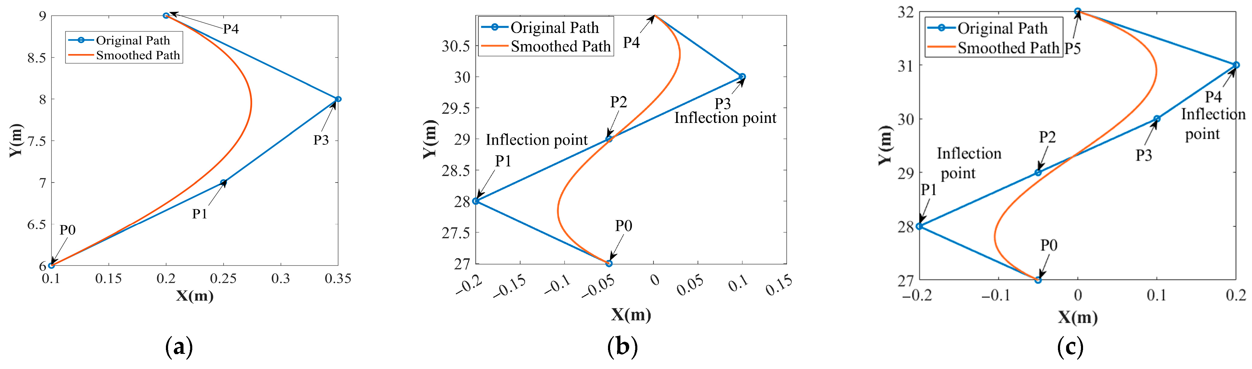
While cubic Bezier curves are generally preferred due to their simplicity and stability, higher-order Bezier curves may be necessary to handle paths with closely spaced inflection points. Specifically, we adopt a combination of third-order Bezier curves, fourth-order Bezier curves, and fifth-order Bezier curves, selecting the appropriate order based on the spacing between inflection points to ensure smoothness and avoid path overlap. The cubic Bezier curves are primarily used for most segments of the path because they offer a balance between stability and flexibility, as shown in Figure 9a. However, when the interval between two inflection points is one path point, a fourth-order Bezier curve is applied to provide additional control, ensuring a smoother transition and eliminating overlaps, as shown in Figure 9b. Similarly, when the interval between inflection points is two path points, a fifth-order Bezier curve is used for smoothing, offering even finer adjustment, as illustrated in Figure 9c.

The path optimization process begins by analyzing the change in heading angle between adjacent nodes, which helps identify significant polylines. For these nodes, additional control points are selected near them, and the appropriate Bezier curve is applied based on the interval between inflection points. Finally, the smoothed road segments are combined with the original path to form an optimized, continuous path. This method ensures a balance between smoothness, obstacle avoidance, and stability while achieving an efficient and safe path in complex environments.

4. Experimental Validation

To validate the effectiveness of the path planning method integrating collision prediction, we designed two experimental platforms: one for path planning in an obstacle-free environment and another for path planning in an environment with obstacles. These platforms were used to experimentally verify the path planning performance and the actual operational results based on the planned paths. To better compare and demonstrate the algorithm’s effectiveness and scalability, we modified the collision detection process of the original A algorithm. Specifically, the collision detection was changed from the original grid occupancy-based method to the collision prediction approach used in this study. This modified process was applied in both operating scenarios. The performance of the proposed path planning method integrating collision prediction was evaluated by comparing metrics such as execution time, path length, and maximum turning angle. Additionally, the safety of the operational process was assessed and analyzed.

4.1. Path Planning Validation in Obstacle-Free Tunnels

4.1.1. Experimental Setup in Obstacle-Free Tunnels

The experiment was conducted to validate the path planning in the coal mine excavation face environment. The environment is obstacle-free scenario. Due to the large size of the excavation machine, it occupies a significant portion of the tunnel space, further restricting the already narrow tunnel, which presents challenges for motion control and potential safety risks. Based on the parameters of the robotic roadheader and tunnel, the motion path planning for robotic roadheader is carried out using the proposed improved A* path planning method integrated with collision prediction. In this process, the performance of path planning is validated by simulating the robot’s actual motion. Both the proposed method and the improved original A* method is used for path planning, with performance analyzed in terms of planning time, path length, maximum turning angle, and safety assessment. Finally, the planning results are applied to the actual tracking control, and the validity of the path planning is verified by monitoring the robot’s actual motion process.

4.1.2. Experimental Scene and Metrics in Obstacle-Free Tunnels

To further validate the practical application of the planned path, we designed a path tracking experiment, as shown in Figure 10. This platform consists of a robotic roadheader, a visual-inertial navigation system [26], and a total station tracking system (IX1000, Beijing Ance Keyi Photoelectric Technology Research Institute, Beijing, China) and PC (i5-8250U, MX150, 8G, Lenovo, Beijing, China). The visual-inertial navigation system, consisting of a visual positioning system and an IMU, is used to monitor the real-time pose of the excavation machine. The total station tracking system is employed to track the real-time position of the excavation machine.

The tunnel parameters used in the experiment are shown in

Table 1. Parameters of tunnel.

Para.	${\mathit{W}}_{\mathit{h}}$/m	${\mathit{H}}_{\mathit{h}}$/m	${\mathit{L}}_{\mathit{h}}$/m	Start Point/m	End Point/m	Depth/m	Section Num
Tunnel	6	3	3000	(0, 0)	(0, 3000)	1.0	20

.

The parameters of the robotic roadheader used in the experiment are shown in

Table 2. Parameters of robotic roadheader.

Para.	${\mathit{W}}_{\mathit{b}}$/m	${\mathit{L}}_{\mathit{c}}$/m	${\mathit{L}}_{\mathit{a}}$/m	${\mathit{L}}_{\mathit{b}1}$/m	${\mathit{L}}_{\mathit{b}2}$/m	${\mathit{W}}_{\mathit{b}\mathit{c}}$/m	${\mathit{\theta }}_{\mathbf{max}}$/°
roadheader	3.5	0.8	4.0	3.25	1.325	1.0	20

.

Based on the pose planning results, the robotic roadheader is controlled to move along the planned path. During the movement, the total station tracking system records the real-time position of the excavation machine, and these position data are compared with the planned path to analyze the practical application of the planned route. The table below lists the equipment and parameters used in the path tracking experiment.

It should be noted that, since the robotic roadheader is unable to complete the cutting in a single pass, we have designed a machine relocation path for the current tunnel. Based on the path point coordinates obtained in the previous sections, six segments of the relocation path were generated: Segment 1: $D_1\left(-0.5 \mathrm{m},5 \mathrm{m}\right)\mapsto O_1\left(-0.67 \mathrm{m},11.2 \mathrm{m}\right)$; Segment 2: $O_1\left(-0.67 \mathrm{m},11.2 \mathrm{m}\right)\mapsto M\left(0 \mathrm{m},6 \mathrm{m}\right)$; Segment 3: $M\left(0 \mathrm{m},6 \mathrm{m}\right)\mapsto O_2\left(0.67 \mathrm{m},11.2 \mathrm{m}\right)$; Segment 4: $O_2\left(0.67 \mathrm{m},11.2 \mathrm{m}\right)\mapsto M\left(0 \mathrm{m},6 \mathrm{m}\right)$; Segment 5: $M\left(0 \mathrm{m},6 \mathrm{m}\right)\mapsto O_1\left(-0.67 \mathrm{m},11.2 \mathrm{m}\right)$; Segment 6: $O_1\left(-0.67 \mathrm{m},11.2 \mathrm{m}\right)\mapsto D_2\left(-0.5 \mathrm{m},6 \mathrm{m}\right)$. The movement along these six segments is shown in Figure 11.

Here, $D_1$ represents the trajectory point before the start of each cutting pass, and $D_2$ is the stop point after completing the current tunnel section cutting, which also serves as the next trajectory point. Typically, the distance between $D_1$ and $D_2$ corresponds to the depth of one tunnel section. The cutting process is performed sequentially, forming a set of trajectory points for tunnel excavation. Precise control of this trajectory ensures the accuracy of the tunnel alignment. In the figure, $O_1$ and $O_2$ are the stopping points after two cutting passes. However, due to the dynamic characteristics of the excavation machine, it is not possible to directly translate from $O_1$ to $O_2$, and thus, an intermediate transfer point is needed. The point M in Figure 11 represents this transfer path point, acting as a bridge between $O_1$ and $O_2$. For ease of control, the excavation machine is assumed to have a heading angle of 0° at these trajectory points, aligning with the designed tunnel direction. This allows for the creation of a complete relocation path, from the initial cutting start point to the cutting completion point, as shown in the figure. The full relocation path of the roadheader can be divided into two parts: $D_1$–$O_1$–M–$O_2$ and $O_2$–M–$O_1$–$D_2$. Although the target points for machine relocation are defined, their exact positions remain uncertain. The determination of cutting location points $O_1$, $O_2$, and the transfer path point M is crucial and forms the basis for planning the relocation path.

4.1.3. Performance of Path Planning in Obstacle-Free Tunnels

Using the previously mentioned tunnel and robotic roadheader parameters, along with the six-segment path of the roadheader, we applied the proposed safety path planning method with collision prediction. The resulting path, compared to the previous method, is shown in Figure 12. The background color bar in the figure represents the artificial potential field values of the environment. The robot’s path is shown with a red line, with solid lines marking the start and end points, and dashed lines illustrating the motion path. Key points on the robot’s outline are also highlighted.

As shown in Figure 12a, both the original and improved path planning methods ensure the safe movement of the robotic roadheader from the starting point. That can be observed from the zoomed-in regions of the left and right images. The key difference is that the boundary points on the left side of the robot in the improved method are further from the tunnel boundary, marked by black circles, indicating a safer path. The improved path also shows smoother motion. In Figure 12b, both methods ensure safe movement, but in the improved method, the left boundary points are farther from the tunnel boundary, suggesting a safer path. Figure 12c shows that, while both methods allow safe movement, the right boundary points of the improved path are farther from the tunnel boundary, indicating a safer path. In Figure 12d, both methods ensure safe movement, but the boundary points on the right side of the robot in the improved path are farther from the tunnel boundary, suggesting greater safety. Figure 12e shows that both methods safely guide the robot, but the boundary points on the left side in the improved method are farther from the tunnel boundary, demonstrating a safer path. Finally, Figure 12f shows that both methods ensure safe movement, but in the improved path, the boundary points on the left are further from the tunnel boundary, again illustrating a safer path.

Furthermore, a performance comparison of the method proposed in this study was conducted, considering factors such as computation time, path length, and maximum turning angle. The results are presented in

Table 3. Performance comparison of the proposed path planning method in obstacle-free tunnels.

Path	Method	Time (s)	ΔT	Length (m)	ΔL	Max Turning Angle (rad)	ΔAngle
$D_1\mapsto O_1$	Before Improved	0.94591	0.8014	6.2122	0.0051	0.1489	0.0857
	After Improved	0.14178		6.2071		0.0632
$O_1\mapsto M$	Before Improved	0.84571	0.7256	5.0812	0.0054	0.1618	0.1044
	After Improved	0.12015		5.0758		0.0574
$M\mapsto O_2$	Before Improved	0.84141	0.7293	5.2627	0.0067	0.1685	0.1110
	After Improved	0.11212		5.2560		0.0575
$O_2\mapsto M$	Before Improved	0.86984	0.7088	5.2622	0.0263	0.1803	0.1191
	After Improved	0.16102		5.2359		0.0612
$M\mapsto O_1$	Before Improved	0.83585	0.7037	5.2607	0.0094	0.1573	0.1122
	After Improved	0.13211		5.2513		0.0451
$O_1\mapsto D_2$	Before Improved	0.75853	0.6429	5.2122	0.0045	0.1489	0.1031
	After Improved	0.11567		5.2077		0.0458

.

As shown in Table 3, compared to the previous path planning algorithm, the improved method reduces the average runtime by 0.7186 s, the average path length by 0.00957 m, and the average maximum turning angle by 0.1059 rad. Therefore, the improved method not only results in a shorter path and reduced computation time but also significantly enhances path smoothness, providing a solid foundation for further autonomous control of the robotic roadheader.

4.1.4. Application of Path Tracker Control of Robotic Roadheader

To better demonstrate the effectiveness of the proposed path planning method in the unobstructed robotic roadheader working scenario, the planned path was applied to the autonomous control of the robotic roadheader. The position and orientation data of the robotic roadheader during its movement were collected using a total station. A comparison between the actual movement and the planned path is shown in Figure 13.

It can be observed that the actual motion paths of the robotic roadheader are generally consistent with the planned path trends, albeit with some deviations. However, these deviations essentially demonstrate the effectiveness of the path planning method. Furthermore, the robot safely reached the designated positions, laying the foundation for carrying out other tasks.

4.2. Path Planning Validation in Obstacle-Filled Tunnels

4.2.1. Experimental Setup in Obstacle-Filled Tunnels

In the underground tunnel environment of coal mines, obstacles often exist that affect the normal passage of robotic systems. Therefore, to ensure safety, obstacle avoidance must be integrated into the robot’s movement to allow safe navigation. Unlike excavation robots, these robots are smaller in size, enabling them to maneuver more freely within the tunnel. Applying the proposed collision-prediction-based path planning method to such scenarios effectively generates safe paths. In the process of simulating the tunnel, the tunnel coordinate system is set up, and the VICON tracking system makes the coordinate system coincide through the initial calibration. Robot motion tracking is achieved by placing marker balls on the robot to create rigid body information. Before the experiment, we set up a narrow and long passage of 0.6 m× 2.5 m, five obstacles at fixed positions, and other information. We then provided different starting points, endpoints, and other controls for the robot to complete path planning and move to the target position. The obstacle coordinates are A (−0.15 m, 0.3 m), B (0.2 m,0.6 m), C (−0.15 m, 1 m), D (0.18 m, 1.5 m), and E (−0.15 m, 2 m).

4.2.2. Experimental Scene and Metrics in Obstacle-Filled Tunnels

To evaluate the obstacle avoidance performance of the path planning method proposed in this study, we designed the experimental validation scenario shown in Figure 14.

In the obstacle-filled experiment, a tunnel with parameters shown in

Table 4. Parameters of tunnels.

Para.	${\mathit{W}}_{\mathit{h}}$/m	${\mathit{H}}_{\mathit{h}}$/m	${\mathit{L}}_{\mathit{h}}$/m	Start Point/m	End Point/m	Depth/m	Section Num
Tunnel	0.6	0.3	3000	(0, 0)	(0, 3000)	1.0	20

was set up, and the robot parameters used in the experiment are provided in

Table 5. Parameters of robot.

Para.	${\mathit{W}}_{\mathit{b}}$/m	${\mathit{L}}_{\mathit{c}}$/m	${\mathit{L}}_{\mathit{a}}$/m	${\mathit{L}}_{\mathit{b}1}$/m	${\mathit{L}}_{\mathit{b}2}$/m	${\mathit{W}}_{\mathit{b}\mathit{c}}$/m	${\mathit{\theta }}_{\mathbf{max}}$/°
roadheader	0.2	0.05	0.05	0.1325	0.1325	0.1	20.0

. Additionally, the equipment used in the experiment includes a mobile robot and a VICON motion capture system. The VICON motion capture system collects the position of the robot’s rigid body, constructed with Induction balls, in the same scene using six industrial cameras. The mobile robot is equipped with an encoder and an STM32f103C8T6 processor (STMicroelectronics NV, Geneva, Switzerland), which transmits the planned results to the robot for tracking control. The validity of the path is verified by comparing the path planning results with the actual tracking results.

4.2.3. Performance Testing

Figure 15a,b show the following: the left images depict the paths generated by the proposed method without optimization, the middle images show the paths with smoothing applied, and the right images present the paths using the weighted A* method. As seen in the figures, applying multiple Bezier curves for path smoothing effectively avoids over-smoothing. The inclusion of obstacle avoidance in the proposed method makes the paths safer near obstacles compared to the improved A* method. To further evaluate the proposed approach, we compared the methods based on running time, path length, average curvature, and maximum turning angle.

Figure 15a shows that both the improved and original path planning methods allow the robot to move from the starting point without collisions. The robot avoids obstacles A, C, and E, and no collisions occur near obstacles B and D, as shown in the zoomed-in view. The main difference is that the path in the right image is smoother.

In Figure 15b, the starting point is closer to obstacle A, but both methods avoid collisions with obstacles A, C, and E. The robot gets close to obstacles B and D, but no collisions occur, as seen in the zoomed view. This highlights the effectiveness of the path planning method, which accounts for the robot’s size constraints.

To further assess the performance of the proposed method, we compared it with the original algorithm based on runtime, path length, and maximum turning angle, as shown in

Table 6. Performance comparison of the proposed path planning method in obstacle-filled tunnels.

Path	Method	Time (s)	ΔT (s)	Length (m)	ΔL (m)	Max Turning Angle (rad)	ΔAngle (rad)
(0.07, 0.15) to (1, 2.1)	Before Improved	3.751	3.483	1.9722	0.0039	0.2971	0.2657
	After Improved	0.268		1.9683		0.0314
(0.02, 0.15) to (1, 2.1)	Before Improved	3.889	3.606	1.9736	0.0052	0.2948	0.2590
	After Improved	0.283		1.9684		0.0358

.

Table 6 shows that the improved method reduces the average runtime by 3.5445 s, the path length by 0.0485 m, and the maximum turning angle by 0.26235 rad, compared to the original algorithm. This results in a shorter path, reduced computation time, and smoother movement. The collision-prediction-based path planning method also provides excellent obstacle avoidance.

4.2.4. Application

The obstacle avoidance path generated by the planning algorithm was applied to the automatic control of a tracked robot in a simulated narrow tunnel, as shown in Figure 16. During the autonomous operation of the robot based on the planned trajectory, the VICON system was used to track the robot’s motion. The resulting trajectory comparison is shown in Figure 16. The parameters of the obstacles, robot, and other settings in the figure are consistent with those in Section 4.2.2.

To validate the planned path, we reduced the robot’s speed to minimize the control system’s impact. As shown in Figure 16a,b, the robot safely reached the target and followed the planned path closely. A comparison of the tracked and planned trajectories revealed a path tracking error, as shown in Figure 16c,d. The maximum errors were 0.0045 m along the x-axis and 0.003 m along the y-axis.

5. Discussion

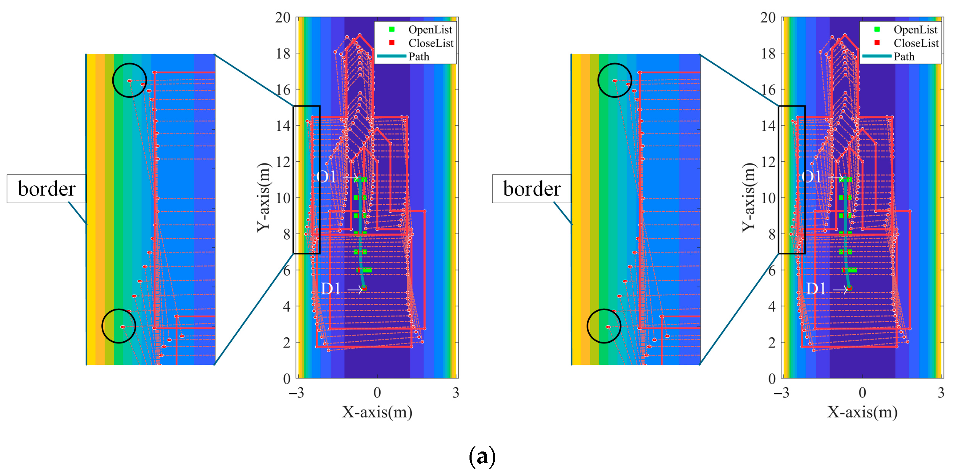
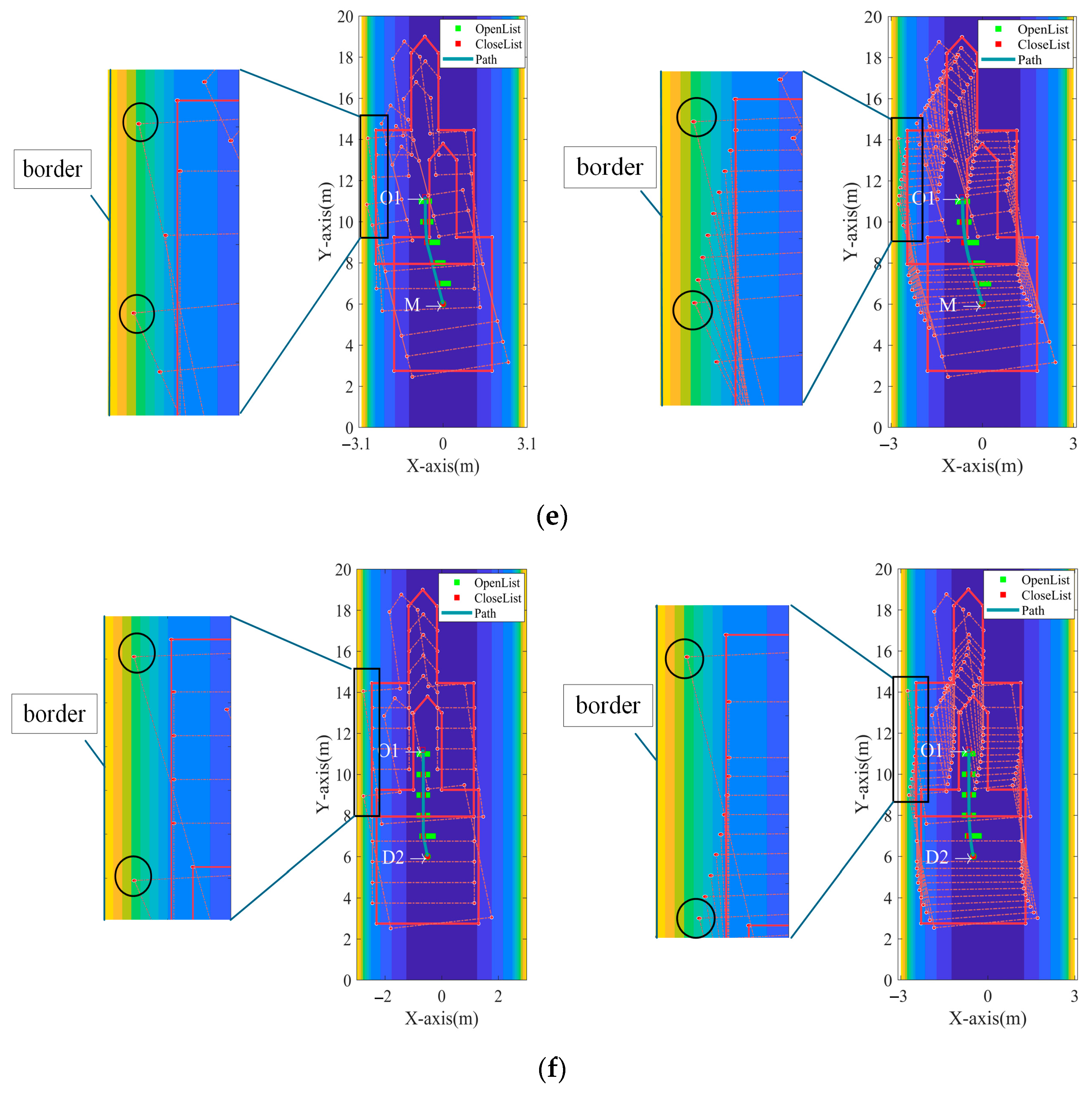
This study presents an optimized path planning algorithm for robotic roadheaders, improving path accuracy in narrow tunnels. Traditional methods often overlook the robot’s dimensions, requiring sensitive perception systems in confined environments. However, the low illumination and high dust levels in coal mine excavation sites make environmental sensing difficult. To address this, we propose an enhanced A* algorithm that incorporates collision prediction, accounting for the robot’s size and other parameters under limited perception. We validated the method in both unobstructed and obstructed scenarios, comparing performance based on computation time, path length, and maximum turning angle. The results show significant improvements over previous methods.

Despite these successes, real-world deployment in tunnels still faces challenges, such as sensor noise, variable tunnel conditions, and the need for real-time adaptation to dynamic environments.

6. Conclusions

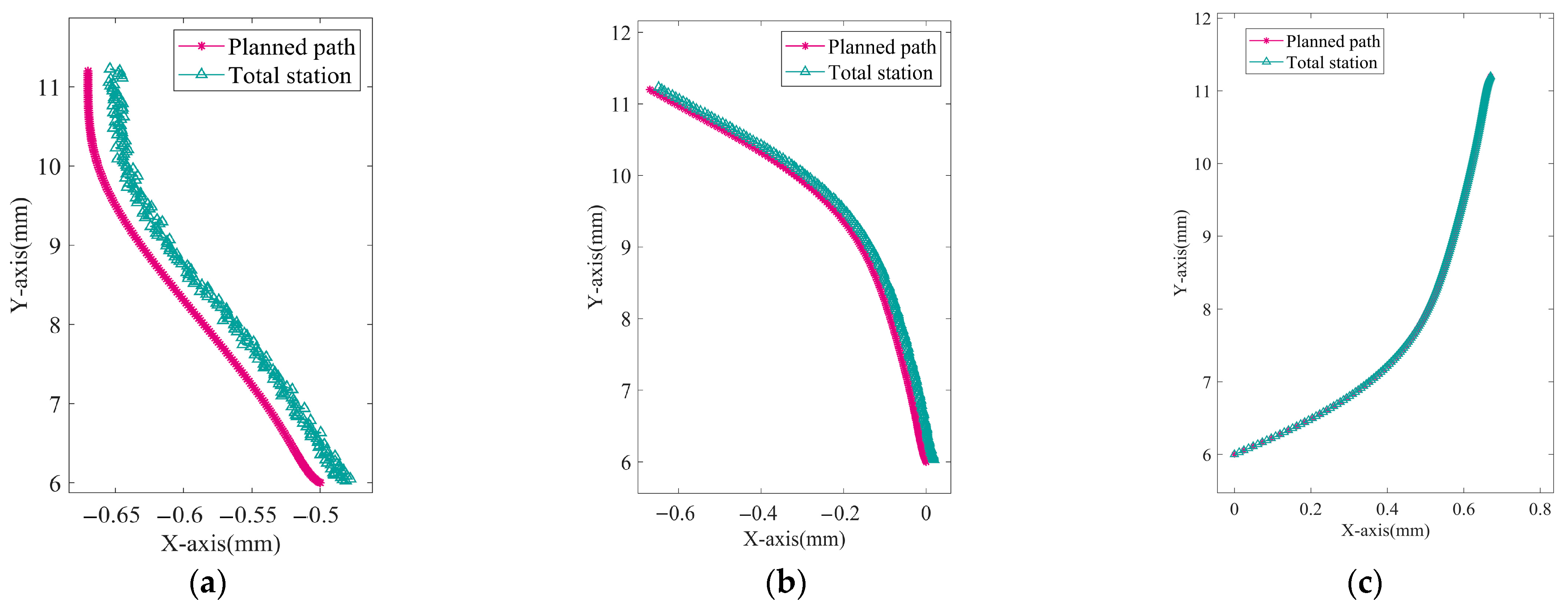
This paper addresses safety and adaptability in path planning for a robotic roadheader in a narrow tunnel. We propose a method that integrates collision prediction with an artificial potential field model, enabling real-time collision detection. The classical A* algorithm is enhanced by a segmented weighted heuristic function and Bezier curve smoothing for safer and smoother paths. We evaluated the method through tests in both obstacle-free and obstacle-filled scenarios with different robot sizes. In the obstacle-free scenario, the method reduced average runtime by 0.7186 s, path length by 0.00957 m, and maximum turning angle by 0.1059 rad. In the obstacle-filled scenario, improvements were more significant, with reductions of 3.5445 s in runtime, 0.0485 m in path length, and 0.26235 rad in turning angle, along with better obstacle avoidance. The planned path also showed a 0.0045 m deviation in tracking control. This method is effective for robotic roadheaders in narrow tunnels and can be extended to other applications, laying a strong foundation for autonomous cutting systems in constrained tunnel spaces.

Future work can extend to more complex tunnel geometries, such as branching structures and steep inclines, to improve the generality of the method. Additionally, the approach can be integrated with the cross-section shaping cutting process to enable a fully autonomous cutting operation, enhancing the overall autonomy and efficiency of robotic roadheaders in mining environments.