An Improved Marriage in Honey-Bee Optimization Algorithm for Minimizing Earliness/Tardiness Penalties in Single-Machine Scheduling with a Restrictive Common Due Date

Abstract

This study evaluates the efficiency of a swarm intelligence algorithm called marriage in honey-bee optimization (MBO) in solving the single-machine weighted earliness/tardiness problem, a type of NP-hard combinatorial optimization problem. The goal is to find the optimal sequence for completing a set of tasks on a single machine, minimizing the total penalty incurred for tasks being completed too early or too late compared to their deadlines. To achieve this goal, the study adapts the MBO metaheuristic by introducing modifications to optimize the objective function and produce high-quality solutions within reasonable execution times. The novelty of this work lies in the application of MBO to the single-machine weighted earliness/tardiness problem, an approach previously unexplored in this context. MBO was evaluated using the test problem set from Biskup and Feldmann. It achieved an average improvement of 1.03% across 280 problems, surpassing upper bounds in 141 cases (50.35%) and matching or exceeding them in 193 cases (68.93%). In the most constrained problems (h = 0.2 and h = 0.4), the method achieved an average improvement of 3.77%, while for h = 0.6 and h = 0.8, the average error was 1.72%. Compared to other metaheuristics, MBO demonstrated competitiveness, with a maximum error of 1.12%. Overall, MBO exhibited strong competitiveness, delivering significant improvements and high efficiency in the problems studied.

1. Introduction

In today’s dynamic global marketplace, optimizing production, administrative, and logistics processes has become essential for organizations seeking not only survival but also growth and prosperity. Competitiveness is continually intensifying, becoming a crucial factor in the viability of any company [1]. In the realm of production and operations management, effectively scheduling tasks on machines is a critical challenge that directly impacts organizational productivity and competitiveness. A particularly complex issue within this domain is single-machine scheduling with a common due date, where both early and late completions incur significant penalties [2]. This challenge is known as the single-machine weighted earliness/tardiness (SMWET) problem. It is a fundamental area of study in production scheduling, which provides a framework for optimizing job sequencing, seeking a balance between delivery times and associated costs. Its relevance extends across various industries (manufacturing, logistics, and services), and advancements in optimization algorithms and techniques continue to expand its applications and utility. As modern production environments become increasingly complex, research in this field remains crucial for enhancing efficiency and competitiveness. The use of SMWET to optimize job sequencing on a production line offers several advantages and disadvantages, which depend on the specific characteristics of the environment and the desired objectives.

The main advantages include the following:

• Simplicity: Scheduling on a single machine is simpler to model and solve compared to multi-machine environments, making implementation and analysis easier. The model incorporates job durations, enabling more accurate planning.
• Flexibility: It allows for the adjustment of penalty weights to prioritize certain tasks, adapting to the specific needs of production or service.
• Resource optimization: Proper scheduling can maximize machine capacity usage, minimizing idle time and improving operational efficiency.
• Improved customer satisfaction: By minimizing penalties for tardiness and earliness, customer relationships can be enhanced by better meeting delivery deadlines.
• Suitable for a critical machine: Optimizes the work sequence in environments where a machine is a key resource.
• The main disadvantages include the following:
• Computational complexity: It is NP-hard, making it difficult to find optimal solutions for large job sets.
• Does not consider multiple machines: It is limited to a single-machine environment, unsuitable for systems with multiple stations.
• Effect of penalties: Penalties for early/late completions must be well-defined for the model to function correctly.
• Complexity in implementation: Although the problem is conceptually simple, implementing a system that considers all constraints and optimizes performance can be complicated.
• Limitation in flexibility: It may not adapt well to dynamic production environments or those with frequent changes.

Scheduling problems are classic discrete combinatorial optimization problems. Most of these belong to the well-known class of just-in-time scheduling, which aims to optimize the supply chain by delivering materials and components precisely when required, minimizing inventory and maximizing operational efficiency [3]. Common due date assignment and just-in-time scheduling have been extensively researched in recent years [4,5].

Due dates are key parameters in scheduling problems. When all jobs share a single due date, it is referred to as a common due date scheduling problem. These dates are determined within the context of the business relationship, considering both client objectives and company goals to ensure customer satisfaction, while minimizing production costs [6]. In a common due date scheduling problem, some jobs may be completed ahead of schedule, while others may be delayed. Early job completion necessitates storage, incurring additional expenses. Late job delivery results in contractual penalties, profit loss, and damage to the manufacturer’s reputation. Both scenarios are unfavorable due to their associated costs and negative impact on the company [7].

Generally, problems involving common due dates can be categorized into two types: restrictive and non-restrictive. Specifically, if the optimal common due date is either a decision variable or does not impact the optimal task sequence, the problem is classified as non-restrictive. Conversely, if the common due date is given and can influence the optimal task sequence, the problem is considered restrictive. In this case, the search for an optimal task schedule must be conducted with respect to the due date [8].

The approaches used in this area are generally categorized into mathematical methods and metaheuristic algorithms [9]. While mathematical methods are effective in situations where gradients can be calculated, they often encounter significant challenges when solving global optimization problems [10]. This limitation has motivated the development of nature-inspired algorithms [11], which have demonstrated remarkable success in addressing optimization complexities on benchmark datasets, such as those published at the IEEE congress on evolutionary computation (CEC).

Widely used across various domains, metaheuristic algorithms have been studied for several decades. These optimization techniques employ nature-inspired simulations and provide high-quality approximate solutions to complex problems that are difficult to solve [12]. To address scheduling problems, there are primarily two types of methods: exact algorithms and approximate algorithms. Exact algorithms mainly encompass mathematical programming, dynamic programming, and branch-and-bound methods. Approximate algorithms primarily include heuristic and intelligent algorithms [13]. Specifically, this study proposes the use of the MBO algorithm, categorized as an approximate metaheuristic algorithm. MBO has emerged as a promising approach for tackling complex problems. Its effectiveness lies in its ability to discover optimal solutions by drawing inspiration from the natural mating process of queen honey bees and drones [14]. There are several algorithms derived from MBO, such as fast marriage in honey-bee optimization (FMHBO), honey-bee mating optimization (HBMO), honey-bee optimization (HBO) and next-generation hybrid algorithms such as hybrid honey-bee simulated annealing (HBSA) [15], the honey-bee mating-based firefly algorithm (HBMFA) [16], and others focused on nectar collection, such as the hierarchical learning-based artificial bee colony (HLABC) [17], the artificial bee colony + particle swarm optimization (ABCPSO) [18], the one-dimensional binary artificial bee colony (oBABC) [19], and the artificial bee colony based on a two-dimensional queue structure (KLABC) [20], among others.

MBO simulates the mating process of honey bees, where queen bees select the most suitable drones to ensure offspring quality. It employs selection and adaptation principles that can be highly effective in optimizing task scheduling [21]. Benatchba et al. [22] propose the use of an artificial bee colony-inspired optimization algorithm to tackle a complex data mining problem framed as a Max-SAT problem. The algorithm proved effective in generating high-quality solutions within reasonable computational limits, outperforming several conventional optimization techniques. Palominos et al. [23] propose an algorithm inspired by honey bee behavior, which incorporates chaotic elements to enhance solution exploration. Empirical results validate the algorithm’s superiority, yielding higher-quality and more efficient solutions than conventional approaches across multiple traveling salesman problem instances. Alotaibi [24] proposes a hybrid algorithm that combines the behavior of artificial bee colonies with that of spiders to optimize resource allocation in the cloud. This problem has grown increasingly complex due to the escalating demands of cloud services. The findings reveal that, in terms of cost, the proposed method outperforms various bio-inspired optimization algorithms.

Recently, Yogeshwar and Kamalakkannan [25] proposed a hybrid MBO-rock hyraxes swarm optimization algorithm for efficient key generation in data sanitization and restoration. This approach significantly improved privacy and security in IoT-based systems by effectively concealing sensitive data during transmission. The model achieved 97% effectiveness on the analyzed dataset, outperforming other compared methods. Xiao et al. [26] introduced an MBO approach for efficient area coverage using swarms of robots, especially in challenging environments. Inspired by bee and ant colonies, the methodology incorporates specific behavioral models for each robot type. The algorithm demonstrated adaptability to dynamic conditions, including unexpected threats, across various experimental scenarios.

The scheduling problem to be solved involves sequencing tasks on a machine to minimize the total penalties associated with early and late deliveries relative to a deadline. The purpose of this study is to develop a schedule that minimizes the objective function value, which represents the cost associated with these penalties. This study adopts the methodology of Abbass [27,28,29], adapted for discrete problems, introducing a novel use of the MBO algorithm that has not been previously explored in this context. The main objective is to evaluate the efficiency of this metaheuristic method in solving NP-hard combinatorial optimization problems, specifically in scheduling.

Related Literature

The general problem of minimizing total penalties for early and late tasks with a common due date has been investigated by different researchers, including Lv et al. [30], who studied a single-machine scheduling problem with proportional job deterioration, focusing on minimizing the total weighted completion time while considering job release times. Their key contributions include identifying dominance properties and deriving both upper and lower bounds for the problem. Furthermore, they propose a branch-and-bound algorithm and several metaheuristic algorithms, such as tabu search, simulated annealing, and the NEH heuristic. Experimental results show that the branch-and-bound algorithm can solve instances with up to 40 jobs within reasonable timeframes. Additionally, the NEH and simulated annealing algorithms were found to be more accurate than tabu search, providing a comparative analysis of the efficiency and accuracy of the different proposed methods. In addition, Shabtay et al. [6] investigated the single-machine scheduling problem with assignable due dates or windows. Their findings suggest that if the due window’s location is unrestricted, the problem can be solved efficiently. Moreover, when the due window’s length is unlimited, the computational time is reduced further. Nevertheless, imposing bounds on either parameter dramatically increases problem complexity, necessitating a pseudopolynomial-time algorithm to address this NP-hard challenge.

Zhang and Tang [31] propose a method for solving the single-machine scheduling problem with flexible delivery dates. They introduced a dynamic scheduling algorithm to address two specific problems. The objective is to minimize a function that considers early work, late work, and flexible delivery dates. For the first issue, they determine the range of delivery dates based on cost coefficients and develop an algorithm that guarantees an optimal solution. For the second issue, they address the allocation of time windows and propose another algorithm that defines the range of delivery dates. Finally, they provide a numerical example to illustrate the feasibility of their proposed algorithms. Li and Chen [32] investigate the optimization of assigning a common due date to multiple tasks. Their primary contribution lies in formulating and solving a scheduling problem that minimizes penalties for weighted early and late completions. The findings suggest that, under specific conditions, this problem can be resolved using a polynomial-time algorithm.

Atsmony and Mosheiov [33] propose a pseudo-polynomial dynamic programming algorithm to address the NP-hard problem of common deadline assignment on a machine. The goal is to minimize the maximum lead/lag costs while maintaining a specified bound on the total job rejection cost. The results demonstrate an efficient implementation that reduces computational effort, allowing problems with up to 200 jobs to be solved in reasonable times. Additionally, they introduce an intuitive heuristic that, after numerical testing, shows small error margins compared to the optimal solution. Qian et al. [34] developed a single-machine scheduling model incorporating important factors like the learning effect, the lead time, and convex resource allocation. Their findings reveal that three distinct objective functions can be formulated and solved, each targeting the minimization of different scheduling costs, including the lead time, delays, and resource expenses. Furthermore, they demonstrate that all the relevant problems can be solved in polynomial time, indicating that efficient algorithms have been developed to address them.

Arik [2] developed a polynomial-time algorithm to address single-machine scheduling with distinct weights for job preemption and tardiness. The objective is to minimize the total cost resulting from the sum of the weighted anticipation and tardiness, along with the assigned common due date. Leveraging the V-shaped property and machine start time, the proposed heuristic consistently delivers superior solutions within reasonable computational bounds, even as problem complexity increases. Tan and Fu [3] address a single-machine scheduling problem aiming to minimize the total costs incurred by job preemption, tardiness, and idle time. They propose a hybrid approach that integrates a custom dynamic programming algorithm, designed to handle the nonconvex idle cost function, with a genetic algorithm (GA) enhanced by restarts and early discarding for sequencing. The results underscore the method’s superior performance and adaptability compared to existing solutions.

Furthermore, Lee and Kim [35] tackled the single-machine SMWET problem using a parallel GA, followed by James [36], who employed a tabu search (TS) algorithm. Notably, neither study incorporated the third property identified by Biskup and Feldmann [37], which states that an optimal sequence of tasks does not necessarily start at time zero. Biskup and Feldmann generated a test problem set for the SMWET problem, solving them with two specific heuristics while considering the three properties outlined in Section 2. The resulting solution values were established as upper bounds for the problem set, providing a benchmark for subsequent research.

Later, Feldmann and Biskup [8] revisited the SMWET problem, employing five distinct metaheuristic approaches: (i) the evolutionary strategy, (ii) simulated annealing, (iii) threshold-accepting algorithms, (iv) the evolutionary strategy with a destabilizing phase, and (v) threshold-accepting algorithms with stabilized search. They benchmarked these metaheuristics against a subset of test problems from their prior work [37]. Subsequently, [38,39,40,41,42,43] also explored the SMWET problem, utilizing the Biskup and Feldmann [37] test suite for a performance comparison.

A literature review reveals a growing diversity of scheduling approaches for single machines, leading to substantial advancements in efficiency optimization and cost reduction. These advancements primarily focus on the lead time (earliness/tardiness) and the assignment of common delivery dates. The reviewed studies address complex problems such as minimizing weighted completion times, assigning flexible delivery windows, and considering factors like task deterioration and learning.

Notable methodological contributions include branch-and-bound algorithms, pseudo-polynomial dynamic programming, and metaheuristics, which have enabled more efficient solutions to NP-hard problems. However, each approach has its limitations and challenges. While some algorithms achieve optimal solutions in reasonable times for small instances, complexity increases significantly with additional constraints or a larger number of tasks, posing an ongoing challenge.

Moreover, despite significant theoretical progress, scalability and the impact of external factors remain areas requiring further attention. The practical application of these methods in real industrial settings has not yet been fully explored. While valuable contributions have been made, it is crucial to focus on testing these methods in more dynamic and complex environments and to explore hybrid approaches that can address some of the current limitations.

The remainder of this document is organized as follows. Section 2 defines the SMWET problem. Section 3 details the MBO metaheuristics. Section 4 outlines the adaptation of the MBO approach to solve the restrictive SMWET problem. Section 5 presents the computational experiments and discusses the obtained results, evaluating the MBO metaheuristic’s performance on the studied problem set. Finally, Section 6 provides conclusions of the study and suggests some future work.

2. Problem Formulation

Punctuality is a fundamental requirement for successful just-in-time implementation. By scheduling tasks with minimal tolerance and defining strict time windows, deviations from the production plan are minimized. This strategy helps reduce in-process inventory, cycle times, and material management costs. In this context, the objective is to find an optimal sequence of tasks, σ, that minimizes the weighted sum of lead and lag times for all tasks. In the problem formulation, a set of tasks j = {1,2,…, n} is given, available to be processed at time zero. Each task j has a processing time $p_j$ and a common due date d that applies to the entire set of tasks. Suspending tasks is not allowed. A task is considered early if its completion time $C_j$ is less than the common due date and tardy if its processing finishes after the due date. Therefore, if the completion time of task j deviates from the due date, either earlier or later, a penalty will be incurred. The rest of the nomenclature is defined as follows: ${\mathrm{\alpha }}_j,$ a penalty for the early completion of job j per unit of time; ${\beta }_j,$ a penalty for the tardiness of job j per unit of time; $E_j,$ the early completion of job j; and $T_j,$ the tardiness of job j.

Earliness and tardiness are calculated as $E_j$ = max{0; −$L_j$} = max{0; d − $C_j$} and $T_j$ = max{0; $L_j$} = max{0; $C_j$ − d}, respectively, for each job j, j = {1,2,…, n}. The unit penalties per unit time of job j for being early or tardy are ${\mathrm{\alpha }}_j$ and ${\beta }_j$, respectively.

The objective is to identify a feasible schedule, S, that minimizes the aggregate earliness and tardiness penalties given a common due date, d.

$$f\left(S\right)=\sum _{j=1}^n{\alpha }_j\left(d-C_j\right)+\sum _{j=1}^n{\beta }_j\left(C_j-d\right)=\sum _{j=1}^n\left({\alpha }_j{E}_j+{\beta }_j{T}_j\right)$$

(1)

The objective function (Equation (1)) refers to the restrictive case, where the common due date is not a decision variable but is given and can influence optimum task scheduling. It is subject to the following conditions:

$T_j$$\ge S_j+P_j$ − d, j = 1,2,…n

$E_j$$\ge d-S_j$$-P_j$, j = 1,2,…n

$S_j+P_j$$\le S_k+$R$(1-x_{jk}$), j = 1,2,…n − 1; k = j + 1,…n

$S_k+P_k$$\le S_j+$R·$x_{jk}$, j = 1,2,…n − 1; k = j + 1,…n

$T_j$$, E_j$$, S_j$ ≥ 0, j = 1,2,…n

$x_{jk}\in$ {0, 1}, j = 1,2,…n − 1; k = j + 1,…n

In the field of operations research and task scheduling theory, it is essential to identify and apply properties that facilitate the optimization of schedules for various types of problems. This study describes key properties of the SMWET problem, which enable the construction of optimal solutions by organizing sequences of tasks under specific conditions and efficiency criteria. Several authors have examined three properties of the non-restrictive version of the SMWET problem [44,45,46,47,48,49,50]. On the other hand, for the problem with a restrictive due date, properties are identified by the methods proposed in [48,50,51], and they can be formulated in a similar way as that proposed by the authors of [8].

• Property 1: In an optimal schedule, there is no idle time between the processing of two consecutive tasks [50].
• Property 2: An optimal schedule exhibits a V-shaped property in the sense that, within the schedule, the advanced tasks are ordered in decreasing order according to the $p_j/{\mathrm{\alpha }}_j$ ratio, and the tardy tasks are sequenced in the increasing order of the $p_j/{\beta }_j$ ratio. The possibility of a straddling job existing in the set of tasks, i.e., a job whose processing starts early and ends tardily, remains open [37].
• Property 3: There exists an optimal schedule in which the following holds true: (i) the first job in the set starts processing at time zero or (ii) a job is completed exactly on its due date [37].

This research addresses the SMWET problem in its restricted form, considering properties 1 and 3 through the application of the MBO metaheuristic using the Abbass procedure [27,28,29]. The objective is to evaluate the effectiveness of this approach for solving NP-hard combinatorial optimization problems. Specifically, the main contribution of this work is the adaptation of the MBO metaheuristic to address the restrictive SMWET problem, demonstrating its suitability for task scheduling. According to the literature review, and as far as we know, there are no existing studies that apply the MBO algorithm to this area.

To evaluate the performance of the proposed MBO metaheuristic approach for the SMWET problem, a set of standard test problems from the literature, as proposed by Biskup and Feldmann [37] and accessible through the OR-Library [52], was solved. In this context, new upper bounds were established for a significant portion of the test instances. Specifically, the adapted MBO algorithm achieved solutions that were at least as good as, or better than, those of the test problem set in 67.14% of cases.

3. MBO Metaheuristics

The MBO metaheuristic was introduced by Abbass in his 2001 paper [27]. Later, the authors of [28,29,53,54] presented modifications and improvements to the initially proposed algorithm.

The MBO metaheuristic is inspired by the social behavior of mating in bee colonies. It is an evolutionary algorithm designed to solve complex combinatorial problems. MBO employs strategies based on searching for neighboring solutions, placing it in the same category as GAs and ant colony optimization.

Abbass [27,28,29] pioneered the modeling of bee mating for optimization problem-solving. Bee colonies consist of queens, drones, workers, and offspring. The process begins with the queen’s nuptial flight, where she mates with multiple drones. The queen stores the drones’ genetic material in her spermatheca. Each egg is fertilized with a random combination from this stored material, creating the colony’s offspring. Workers tend to the young.

The MBO metaheuristic simulates the mating process of bees as a series of state transitions. Initially, a queen bee’s genotype is randomly generated. Worker bees, acting as local search heuristics, improve this initial solution. Subsequently, the queen embarks on multiple mating flights. Each flight involves the random initialization of the queen’s energy and speed. As she transitions through different states (potential solutions), she has opportunities to mate with randomly generated drones. Successful matings, determined by factors like the queen’s energy and the drone’s fitness, result in the drone’s genetic material being stored in the queen’s spermatheca. After each flight, the queen generates new offspring by combining her genetic material with randomly selected material from the spermatheca. These offspring are refined by worker bees. The fittest offspring replaces the queen, and the process iterates.

The MBO algorithm comprises three core processes: (i) the queen’s mating flight for parent selection, (ii) the creation of offspring through genetic recombination, and (iii) the refinement of offspring by worker bees using local search heuristics [53]. Each process is crucial for the algorithm’s performance in finding optimal solutions.

The MBO algorithm in [27] employs a pure exploration strategy, accepting as many queen paths as possible. Each queen is initially assigned random energy $E_0$ and speed $S_0$ values between 0.5 and 1.0 to facilitate an average of 7–17 matings per flight [27,28,29]. During the flight, the queen’s energy and speed diminish according to Equations (2) and (3).

$$E\left(t+1\right)=E\left(t\right)-g$$

(2)

$$S\left(t+1\right)=\alpha \cdot S\left(t\right)$$

(3)

where parameters $g$ and α correspond to the reduction factors of the queen’s energy and speed at instant t, respectively.

The queen’s energy and speed parameters mimic natural bee behavior. Energy correlates with flight duration, limiting the queen’s search for drones in the solution space. Speed influences mating success, with higher speeds increasing the likelihood of successful mating, especially at the flight’s onset [27,28,29].

The success of a queen’s mating flight depends on the proximity of drones. Drones closer to the queen have a higher mating probability, as defined by Equation (4). These drones are preferentially selected for genetic recombination.

$$p\left(q,d\right)=mín\left\{1,e^{-{\displaystyle \frac{l(q,d)}{s\left(t\right)}}}\right\}$$

(4)

where l(q,d) = dist(f(q), f(d)) is the distance between the evaluations of the fitness functions of the queen and of the drone, and s(t) is the queen’s speed at instant t.

In Abbass’s MBO algorithm [27], queen bees randomly select drones for mating. A drone is accepted as a parent if its mating probability exceeds a random value between 0 and 1. Half of the drone’s genetic material is then incorporated into the queen’s spermatheca, signifying a successful mating.

A mating flight concludes when the queen’s energy depletes, i.e., E(t) = 0, or the spermatheca is full. Upon returning to the hive, the queen initiates reproduction by randomly selecting a drone’s genetic material from her spermatheca for crossover. The resulting offspring undergo mutation by worker bees, finalizing the brood-raising process.

The fittest brood replaces the weakest queen. The remaining broods are discarded. The process iterates until the termination criteria are met.

4. MBO Algorithm for Solving the SMWET Problem

There are two commonly used methods to represent solutions to the SMWET problem [43]. One approach utilizes permutation chains to depict the physical task sequences. Consequently, an SMWET problem with n tasks yields a solution space comprising n permutations. Alternatively, solutions can be sought within a smaller solution space exclusively containing those that inherently satisfy property 2 (the V-shaped property).

This work employs permutation chains for solution representation due to their adaptability and guaranteed feasibility. Accordingly, each genotype (queen, drone, and brood) is characterized by a permutation sequence of equal length (n) representing the task order. Furthermore, a starting time is assigned to each genotype’s initial task, addressing property 3 of the SMWET problem, which stipulates that the first processed task may not necessarily commence at time zero.

4.1. Parameters Used for the MBO Algorithm

In the proposed MBO algorithm, the use of fixed parameters was considered for solving all the instances contained in the set of test problems proposed by the authors of [37], with the purpose of evaluating the effectiveness of the algorithm in the search for good solutions of the problem, and to validate a general solving algorithm in which it would not be necessary to adjust the parameters to solve a particular problem.

The general parameters employed in the proposed algorithm are as follows: (i) The number of queen bees (Q)—this parameter represents the number of queen bees initiating mating flights. The algorithm utilized four queens, each proposing a distinct solution at every iteration. (ii) The number of drones (D)—indicating the maximum number of drones a queen can mate with per flight, D was experimentally fixed at 10. (iii) The spermatheca capacity (M)—this parameter defines the queen’s genetic material storage capacity post-flight. Based on Abbass’s recommendations [27,28,29] suggesting a range of 7 to 17, M was set to 10.

Table 1. Parameters of MBO algorithm.

	Parameter	Source	Value
1	Number of queen bees	Experimental	4
2	Number of drones	Experimental	10
3	Initial speed of the queen bees	[27,28,29,53,54]	0.9
4	Initial energy of the queen bees		0.9
5	Energy reduction factor of the queen bees	[53]	$g$
6	Speed reduction factor of the queen bees	Experimental	0.98
7	Spermatheca capacity	[27,28,29]	10
8	Number of flights	Experimental	20

shows the values of the specific parameters used in the MBO algorithm proposed in this study.

Equation (5) was used to determine the value of parameter 5.

$$g={\displaystyle \frac{0.5\cdot e_0}{M}}$$

(5)

where $e_0$ = E(t = 0) is the initial energy of the queen bee, and M is the size of the spermatheca. The specification of parameter 5 ensures that each queen mates with the amount of drone-derived material stored in her spermatheca.

The values $s_0$ = 0.9 and $e_0$ = 0.9 were chosen for the initial velocity and the queen bee’s energy, respectively, in accordance with the studies [27,28,29,53,54].

4.1.1. Obtaining an Initial Population

This paper examines four queen bees, two initialized with random solutions and two derived from the LPT and SPT scheduling rules. Randomizing half the queen bees fosters greater solution diversity, following the guidelines of [27,28,29,53,54,55]. Each generated queen bee is assigned initial energy and speed parameters. To ensure quality solutions, the initial queen bees are refined using worker bees, which are local search algorithms or simple heuristics.

The initial drone population is also generated randomly, adhering to the original MBO algorithm framework by the authors of [27,28,29].

4.1.2. Mutation of Drones

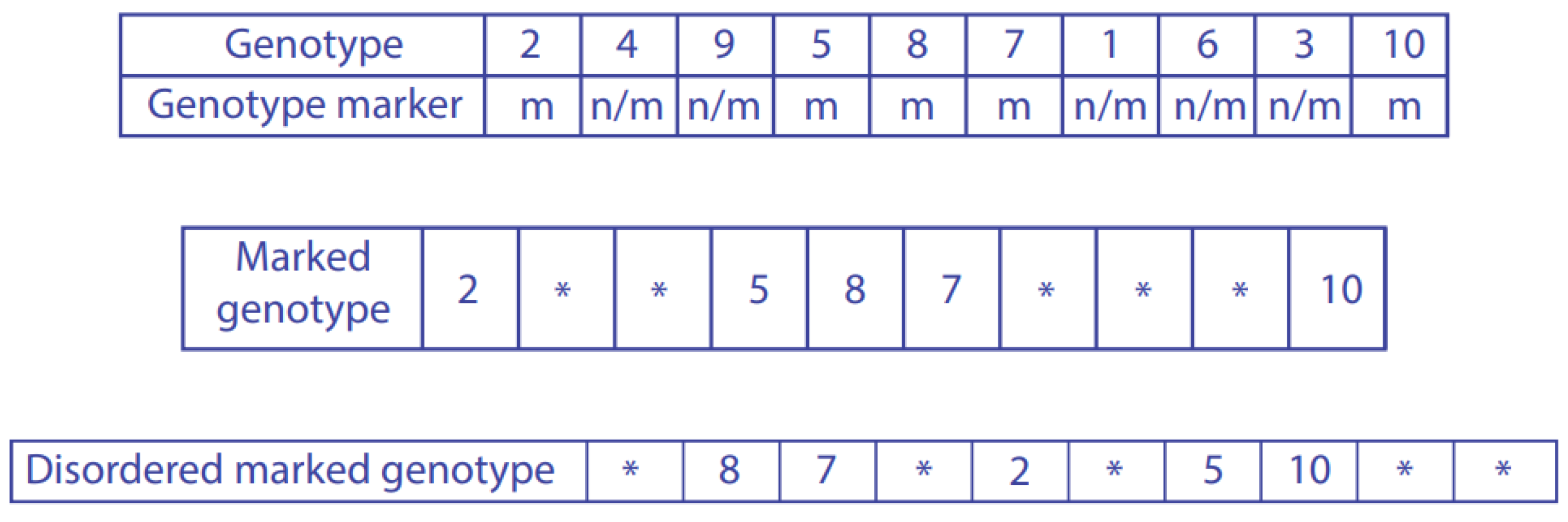
As in [53], each drone should mutate at the time of coupling with the queen. In the mutation process, each drone possesses a genotype, and an operation called a genotype marker (GM). This marker randomly selects half of the drone’s genes for mutation, ensuring that only these genes participate in the creation of brood due to the haploid nature of drones [27,28,29,53,54]. The mutation process involves applying the GM to the drone genotype and then randomly rearranging the marked genes, which will contribute to the offspring.

Figure 1 visually depicts the drone genotype, the GM operator, and the mutation process. The symbol m indicates a marked gene, n/m an unmarked gene, and an asterisk * a non-existent gene.

In this way, at each transition, starting with the original drone genotype denoted by $S_D$, a mutated genotype $S_D^{\mathrm{\prime }}$ is obtained. If the fitness of the mutated drone is higher than that of the original drone (i.e., f($S_D^{\mathrm{\prime }}$) < f($S_D$)), then the mutated drone replaces the original one $S_D$ = $S_D^{\mathrm{\prime }}$.

4.1.3. Selection of the Drone’s Genetic Material

In the implementation of the MBO algorithm for the SMWET problem, it was defined, following [27,28,29,53,54], that the queen probabilistically adds drone material to her spermatheca according to the annealing function presented in Equation (4). A random number between 0 and 1 is generated for each queen and then compared to the highest mating probability of any drone with respect to that queen. If the mating probability is greater than the generated number, the queen bee accepts the drone as a parent, meaning that half of the drone’s genetic material (given its haploid donor status) is added to the queen’s spermatheca, resulting in a successful mating.

Furthermore, in this work, the substitution of a queen by a drone was considered if the fitness of any drone was superior to that of a queen.

4.1.4. Crossing of Genetic Material and Offspring Production

During the mating process, the queen bee stores the genetic material of a drone in her spermatheca. This genetic material is then randomly selected to fertilize eggs, resulting in the creation of broods.

A genetic crossover operator is employed to facilitate the exchange of genetic material between the queen and the drone. This operator selects two individuals, referred to as Parent 1 and Parent 2, and performs a genetic crossover between their genotypes.

The crossover process involves combining the genetic information from both parents to generate a new offspring. The head of the offspring’s genotype sequence is inherited from Parent 2, while the tail is inherited from Parent 1.

The genetic crossover operator can be formally defined by the following three steps: (i) a segment of the cord, which carries the genotype of Parent 1, is randomly selected. This segment is defined by its starting position, i, and ending position, j, where 1 < i < j < n. The genes within this segment (i.e., i, j) are stored as a list. (ii) Genes from Parent 2 are selected, ensuring they are not present in the previously chosen segment of Parent 1. These selected genes are stored in a list of length less than n, where n is the total number of tasks. (iii) The genes from Parent 2 stored in the previously generated list, up to position i (the starting point of the Parent 1 segment), are combined with the Parent 1 segment and the remaining genes from Parent 2, thus creating a new offspring.

The queen’s and drone’s genotypes served as Parent 1 and Parent 2. The crossover operator was applied to create broods with (i) queen-dominant genotypes—the majority of genetic material at the beginning of the sequence was from the queen (with the drone’s genotype as Parent 1 and the queen’s as Parent 2)—and (ii) drone-dominant genotypes—the majority of genetic material at the beginning of the sequence was from the drone (with the queen’s genotype as Parent 1 and the drone’s as Parent 2).

Experiments were conducted using the crossover operator with the drone as Parent 1 in 70% of cases and the queen as Parent 1 in 30%. This approach was based on the general superiority of the queen’s genotype (due to prior optimization) and its potential alignment with the solution structure.

4.2. Improvement of Offspring Using Workers

To address the SMWET scheduling problem, the MBO algorithm was used, employing three heuristics as workers. These heuristics were used to enhance the initial queen bee population and the offspring generated through the genetic recombination of the drone and queen. The specific heuristics utilized were hill climbing, simulated annealing, and a local search operator.

4.2.1. Hill-Climbing Heuristic

Beginning with an initial state or solution, a local search algorithm explores the search space by moving to neighboring states, which enhances the value of a specified objective function [56]. At each iteration, the algorithm modifies one or more elements of the current solution, represented by a vector x, which can contain continuous and/or discrete data. It then assesses how these changes impact the value of the objective function f(x) [57]. This optimization process continues until no neighboring states yield a better solution, leading to a local maximum or minimum, or until a predetermined termination criterion is fulfilled. Algorithm 1 shows the pseudo-code of the hill-climbing heuristic [58].

Algorithm 1. Pseudo code for hill-climbing algorithm
i = initial solution
While f(s) ≤ f(i) for all s $\in$ Neighbors (i) do
	Generates an s $\in$Neighbors (i);
	If fitness (s) > fitness (i) then
		Replace s with the i;
	End If
End While

This search process was selected as a worker based on the suggestion in [27,28,29] to use local search algorithms as workers. The choice of this heuristic and its representation was influenced by the study of M’Hallah [59]. This technique, along with simulated annealing, was chosen due to its ease of application to various combinatorial optimization problems. Despite the risk of converging to local optima, it can provide strong initial solutions.

The hill-climbing heuristic consists of the following three steps: (i) Selecting a starting point or current state $S_i$, which corresponds to the current solution. (ii) Perturbing the current solution ($S_i$→$S_i^{\mathrm{’}}$) and accepting any transition that improves the solution (either upward or downward, depending on the problem’s objective). (iii) Choosing the best successor $S_j$ in the neighborhood of $S_i$, where $S_j$ = best {$S_i^{\mathrm{’}}$}; if there are multiple equally good successors, one is chosen at random.

Transitions are generated by creating neighboring solutions using a task-swapping operator. This operator randomly exchanges tasks within the solution delivered by the brood. If the resulting solution is better than the current one, it is accepted.

4.2.2. Simulated Annealing Heuristic

Stochastic search method inspired by the annealing process in metallurgy, suggested by the authors of [60], and proposed by the authors of [61]. While simulated annealing does not guarantee finding an optimal solution, it can effectively escape local minima by exploring the search space through random movements, particularly in complex environments [62]. This enables suboptimal solutions to improve by employing a decreasing parameter known as “temperature” [63]. Furthermore, simulated annealing is simple to implement and requires minimal parameter tuning, making it well-suited for a wide range of optimization problems, both combinatorial and continuous ones.

This method was chosen as the second worker heuristic due to its versatility and applicability to combinatorial optimization problems. Its probabilistic acceptance of solutions, even if they are not always superior, allows for the exploration of the solution space and avoids the local optima trap, a significant disadvantage of hill climbing. To adapt simulated annealing to our problem, we followed a similar approach as described in [8]. The simulated annealing metaheuristic used in this study, both to refine brood solutions and improve initial queens, is outlined below.

Starting from an arbitrary solution (initial) $S_i$, a solution $S_j$ is chosen randomly in the neighborhood of $S_i$,. Let ${\Delta }_{ij}$ = f($S_j$) − f($S_i$) be the difference between the values of the objective function of $S_j$ and $S_i$. If the value of the objective function of the new solution $S_j$ is less than or equal to the previous ${\Delta }_{ij}$ ≤ 0, then the new solution, $S_j$, becomes the present one and the search process continues from $S_j$. On the other hand, if the objective value of the neighboring solution $S_j$ is greater than the objective value of the previous ${\Delta }_{ij}$ > 0 solution, then $S_j$ is accepted as the present solution with probability $e^{-{\Delta }_{ij}/C_k}$, where $C_k$ represents the present value of the control parameter of the simulated annealing algorithm, which is the temperature. The algorithm begins with a relatively high temperature value, so at the beginning, most of the lower neighboring solutions are accepted. During the execution of the simulated annealing algorithm, $C_k$ remains constant over several iterations and then drops, so the probability of accepting neighboring solutions is less in the terminal stage of the search process. The present work considered an initial temperature $C_{k=0}$ = 0.9, which remains constant over several iterations equal to $L_k$ = 8. A linear type of temperature reduction function and a temperature reduction factor (or cooling factor) c = 0.8 were also used, so that the temperature after each transition decreased according to the rule $C_k$ = c $C_{k-1}$. The simulated annealing algorithm (Algorithm 2) can be outlined as follows.

Algorithm 2. Pseudo-code for simulated annealing algorithm
Step 0: k: = 1, $S_i$: = $S_{star}$, $S_i$: = $S_{best}$, $c_1$: = $c_{star}$
Step 1: Select at random $S_j$$\in$N ($S_i$)
	If ${\Delta }_{ij}$≤ 0 then: $S_i$: = $S_j$ and if f($S_i$) < f($S_{best}$) then $S_{best}$: = $S_i$
		else: If exp(−${\Delta }_{ij}$/$c_k$) > random [0, 1) then $S_i$: = $S_j$
Step 2: After $L_k$ repetitions of Step 1: $c_{k+1}$: = $g$($c_k$) and k: = k + 1
Step 3: If stop criterion is not true go to Step 1

Like hill climbing, transitions are generated by creating neighboring solutions using a swap operator. This operator randomly exchanges tasks within the solution provided by the brood. Solutions are accepted if they improve the current solution or meet the simulated annealing acceptance criteria, based on a predetermined number of iterations. The best solution found throughout the process is retained and presented as the final output.

4.2.3. Local Search Operator

In addition to the two heuristic workers, it was decided to use a swap operator that works in parallel to these workers. A local search operator makes minimal changes to the current solution with the goal of improving its quality [64]. This operator is based on the findings of Pan et al. [39], who also investigated the SMWET problem. To further enhance solution quality, these authors applied an iterative local search to the global best solution $G^t$. This search utilizes a simple binary exchange neighborhood. The local search procedure involves swapping two randomly selected tasks, subject to the condition that the first of these tasks is early with respect to the due date and the second is tardy with respect to the due date. This task-swapping operator was also introduced by the authors of [8]. The iterative local search in Algorithm 3 was based on the simple binary swap neighborhood.

Algorithm 3. Pseudo-code for Iterated local search algorithm
s0 = Gt$s_0$= $G^t$
s = Local Search ($s_0$)
Do{
	$s_1$= Perturbation (s)
	$s_2$= LocalSearch ($s_1$)
	s = AcceptanceCriterion (s, s2)
}While (Not Termination)
If f(s) < f($G^t$) then $G^t$= s

In this work, both the heuristic and task-swapping operators are initially used to refine the initial queens and later used to enhance the offspring produced through the genetic recombination of the queen and drone. The selection of the candidate heuristic is performed probabilistically in three steps: (i) Each heuristic candidate is assigned a selection probability. The heuristic with the highest probability after each iteration is chosen as the worker. Initially, all heuristics have a probability of 1/w, where w the total number of workers. (ii) The average improvement $\left({\overline{imp}}_h\right)$ achieved by each heuristic h is calculated and stored. This represents the average improvement of the brood solution. (iii) The selection probability is then updated to reflect the impact of the most effective heuristic. The new probability, $p^{\mathrm{\prime }}$, is calculated as the previous probability p plus the ratio of the average improvement contributed by heuristic h to the sum of all average improvements and the total number of workers w. This calculation ensures that the new probability remains between 0 and 1. Formally, the new choice probability is given by Equation (6).

$$p^{\mathrm{\prime }}=p+{imp}_h/\left(\sum \overline{imp·w}\right)$$

(6)

The choice rule defined in Equation (6) is applied after each iteration of the heuristics, selecting the one with the highest choice probability. Once selected, each solution improvement method is executed a specific number of times: 200 iterations for simulated annealing, 50 iterations for hill climbing, and 40 iterations for local search. These iteration values were determined experimentally.

4.3. Population Updating

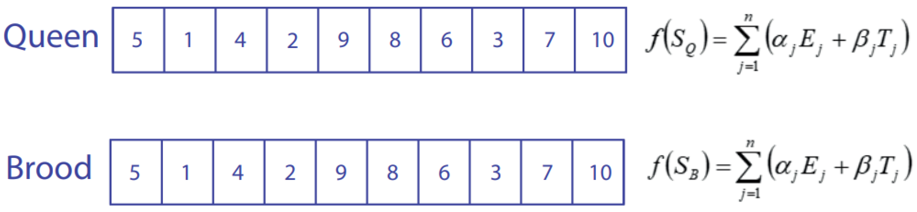
In each flight, after the broods obtained from crossing operations have been improved through the application of worker heuristics, the fitness of the newly improved broods is evaluated. If the fitness function of an improved brood is better than the fitness function of some queen, f($S_B^{\mathrm{’}}$) < f($S_Q$), then the queen population is updated by removing the least fit queen and replacing her with the brood that has the best fitness, $S_Q$ = $S_B$.

The evaluation function determines whether the newly generated individual (the improved brood) is suitable to be considered a new solution-generating individual (queen bee).

Therefore, the proposed MBO algorithm evaluates both queens and broods using Equation (1), applied to the partial solutions of each: f($S_Q$) for queens and f($S_B$) for broods. Figure 2 provides a schematic representation of the fitness evaluation process.

At the end of each flight, the queen population is updated by replacing the queens with the worst fitness with broods that have the best fitness, if any exist. The lists of generated broods and drones are then deleted. A new population of drones is generated for the subsequent flight, resulting in new broods from crossing the genotypes of the queens and the new drones.

This process is repeated until the algorithm’s stopping condition is met. Since queens are updated after each flight, the algorithm iterates through all the previously mentioned stages until the stopping criterion is fulfilled.

4.4. Parameter Updating

During each mating flight, a queen bee experiences a loss of energy, a decrease in flight speed, and a reduction in available space in her spermatheca. To accurately simulate these changes, parameters related to the queen’s energy, speed, and spermatheca capacity must be updated after each flight. The updating procedure follows the methods outlined by the authors of [27,28,29,53,54]. In this way, the relevant parameters updated during each flight are as follows.

• Updating the queen’s energy: This is completed using Equation (2): E(t + 1) = E(t) − $g$. At each transition t, the energy is reduced by $g$ units, where $g$ corresponds to the energy reduction factor of the bees, as previously described in Equation (5).
• Updating the queen’s speed: This is completed using Equation (3): S(t + 1) = α∙S(t). At each transition t, the speed is progressively reduced by a factor α of the previous speed.
• Updating the spermatheca’s capacity: The capacity of the spermatheca is updated based on the number of drones with which the queen mates during each flight. This depends on the acceptance or rejection of the mating event between the queen and the drone, which is represented by the annealing probability described in Equation (4).

4.5. Stopping Conditions

In the implementation of the MBO algorithm, a stopping criterion was established based on reaching a predetermined number of iterations, equivalent to the number of flights. For the scheduling problem examined, it was determined that 20 flights within the MBO algorithm yielded satisfactory solutions for a substantial portion of the 280 problems investigated. Consequently, this number of flights was considered suitable for addressing the SMWET problem. The MBO metaheuristic proposed for the SMWET problem is described in Algorithm 4.

Algorithm 4. Queen–brood fitness evaluation

Define

M, (to be spermatheca size); Q = 4, (queen quantity); α = 0.98, (queen velocity’s reduction step)

Define

E(t) and S(t) to be the queen’s energy and speed at time t, respectively

Define

maxiter_hc, maxiter_sa, maxiter_ls to be the maximum number of iterations for workers

Initialize

workers to be simulated annealing, hill climbing and local search.

Initialize

queen genotypes, according to SPT and LPT scheduling rules for the first two queens and randomly

generate the genotypes for the remaining two queens.

Randomly use workers to improve initial queen’s genotype

while

Flight quantity < 20:

t = 0

Initialize

$e_0=0.9$$; s_0$$=0.9 \mathrm{and} g$ = [0.5 E(t)/M]

Generate D = 10 drones at random

while

E(t) > 0 and M < 10: (queen still have energy to flight and spermatheca is not full)

Mutate drones genotype $S_D$→$S_D^{\mathrm{\prime }}$

if, f$(S_D^{\mathrm{\prime }}$$) < f(S_D$)

(if mutated drone fitness is better than the original drone fitness, then accept mutated drone genotype as potential drone)

$\to S_D$$=S_D^{\mathrm{\prime }}$

else if, f$(S_D^{\mathrm{\prime }}$$) < f(S_Q$)

(if mutated drone fitness is better than queen fitness, replace queen genotype by mutated drone genotype)

$\to S_Q$$=S_Q^{\mathrm{\prime }}$

end if

end elseif

Select the candidate drone’s genotype to cross it with the queen’s genotype according with annealing probability, (Equation (4))

if, rand$\left(0.1\right) < p\left(qd\right)\to M \mathrm{\prime }$ $=\{S_D$$, S_D^{\mathrm{\prime }}$} for D = {1, 2,…, 10}

(add drone’s genotype to spermatheca)

t = t + 1; E(t + 1)=E(t) − $g$; S(t + 1) = αS(t)

end while

for brood

=1 to total number of broods

select drone material from queen spermatheca at random

if rand(0.1) ≤ 0.3 apply “drone-queen” crossover operator and generate a brood

else, apply “queen drone” crossover operator and generate a brood

endif

use workers to improve brood’s genotype according to the probabilistic rule (Equation (6))

for workers [hill climbing, simulated annealing and local search]

$\mathrm{determine} p_{best}$, the best election probability associated with a worker

select worker

apply worker to all broods to obtain mutated broods

$S_B$$\to S_B^{\mathrm{\prime }}$

$\mathrm{Actualize} p_{best}$

end for

if f$(S_{B }$$) > f(S_B^{\mathrm{\prime }}$)

(if mutated brood fitness is better than the original brood fitness, then keep mutated brood as partial solution)

$\to S_B$$=S_B^{\mathrm{\prime }}$

end for

if f$(S_{Q }$$) > f(S_B$)

(if there are broods with better fitness than any queen, replace the queen by broods)

$\to S_Q$$=S_B$

end if

kill all broods

end while

The flowchart of the MBO algorithm, adapted for this study, is provided in Figure 3.

5. Computational Experiments and Results

5.1. Benchmarks Used for Experimentation

The MBO algorithm for addressing the SMWET problem was implemented in Python. The algorithm was evaluated using a suite of test problems developed by the authors of [37] and is accessible in the OR-Library [52]. This collection comprises a total of 280 benchmark problems, spanning seven categories with n = 10, 20, 50, 100, 200, 500, and 1000 tasks, with 10 problems in each category. For each problem, a due date restrictiveness factor h = 0.2, 0.4, 0.6, and 0.8 was considered.

The common due date value is generated by d = [h∙∑$p_j$], meaning that, for each problem, the common due date is estimated by multiplying the restrictive factor h by the sum of the processing times ($p_j$) of the n tasks. Thus, the smaller the value of h, the more restrictive the problem becomes.

The results are analyzed by comparing the values obtained by the proposed MBO metaheuristic with the upper bound (UB) values provided by the authors of [37], who used two specific heuristics for the problem. Additionally, the effectiveness of the MBO metaheuristic is compared with other metaheuristic techniques found in the literature that have been applied to the SMWET problem using the same set of test problems [8,38,39,40,41,42,43].

The performance of the MBO algorithm is assessed using the percent error index, which compares the solutions obtained by the MBO algorithm (referred to as the obtained MBO value) with the UB provided by the authors of [37] (denoted as ${UB}_{F\&B}$). This index is calculated using Equation (7).

$$percent⥂\hspace{0.33em}⥂error\hspace{0.33em}=\hspace{0.33em}{\displaystyle \frac{(obtained\hspace{0.33em}MBO\hspace{0.33em}value-U{B}_{B\&F})}{U{B}_{B\&F}}}\times 100\%$$

(7)

5.2. Results Obtained on the Benchmarks from [37]

Table 2. Results for n = 10, 20, and 50.

		h = 0.2			h = 0.4			h = 0.6			h = 0.8
n	k	UB	MBO	% Offset	UB	MBO	% Offset	UB	MBO	% Offset	UB	MBO	% Offset
10	1	1936	1936	0.00	1025	1025	0.00	841	841	0.00	818	818	0.00
	2	1042	1042	0.00	615	615	0.00	615	615	0.00	615	615	0.00
	3	1586	1586	0.00	917	917	0.00	793	793	0.00	793	793	0.00
	4	2139	2139	0.00	1230	1230	0.00	815	815	0.00	803	803	0.00
	5	1187	1187	0.00	630	630	0.00	521	521	0.00	521	521	0.00
	6	1521	1521	0.00	908	908	0.00	755	755	0.00	755	755	0.00
	7	2170	2170	0.00	1374	1374	0.00	1101	1101	0.00	1083	1083	0.00
	8	1720	1720	0.00	1020	1020	0.00	610	610	0.00	540	540	0.00
	9	1574	1574	0.00	876	876	0.00	582	582	0.00	554	554	0.00
	10	1869	1869	0.00	1136	1136	0.00	710	710	0.00	671	671	0.00
		Average		0.00	Average		0.00	Average		0.00	Average		0.00
20	1	4431	4394	−0.84	3066	3066	0.00	2986	2986	0.00	2986	2986	0.00
	2	8567	8430	−1.60	4897	4847	−1.02	3260	3206	−1.66	2980	2980	0.00
	3	6331	6210	−1.91	3883	3838	−1.16	3600	3583	−0.47	3600	3583	−0.47
	4	9478	9188	−3.06	5122	5118	−0.08	3336	3317	−0.57	3040	3040	0.00
	5	4340	4215	−2.88	2571	2495	−2.96	2206	2173	−1.50	2206	2173	−1.50
	6	6766	6527	−3.53	3601	3582	−0.53	3016	3010	−0.20	3016	3010	−0.20
	7	11,101	10,455	−5.82	6357	6238	−1.87	4175	4126	−1.17	3900	3878	−0.56
	8	4203	3920	−6.73	2151	2145	−0.28	1638	1638	0.00	1638	1638	0.00
	9	3530	3465	−1.84	2097	2096	−0.05	1992	1965	−1.36	1992	1965	−1.36
	10	5545	4979	−10.21	3192	2925	−8.36	2116	2110	−0.28	1995	1995	0.00
		Average		−3.84	Average		−1.63	Average		−0.72	Average		−0.41
50	1	42,363	40,697	−3.93	24,868	23,792	−4.33	17,990	17,969	−0.12	17,990	17,937	−0.29
	2	33,637	30,624	−8.96	19,279	17,920	−7.05	14,231	14,054	−1.24	14,132	14,200	0.48
	3	37,641	34,425	−8.54	21,353	20,502	−3.99	16,497	16,509	0.07	16,497	16,591	0.57
	4	30,166	27,755	−7.99	17,495	16,657	−4.79	14,105	14,121	0.11	14,105	14,215	0.78
	5	32,604	32,307	−0.91	18,441	18,007	−2.35	14,650	14,612	−0.26	14,650	14,618	−0.22
	6	36,920	34,969	−5.28	21,497	20,385	−5.17	14,251	14,274	0.16	14,075	14,116	0.29
	7	44,277	43,134	−2.58	23,883	23,038	−3.54	17,715	17,637	−0.44	17,715	17,682	−0.19
	8	46,065	43,859	−4.79	25,402	24,892	−2.01	21,367	21,403	0.17	21,367	21,435	0.32
	9	36,397	34,234	−5.94	21,929	19,986	−8.86	14,298	14,202	−0.67	13,952	14,056	0.75
	10	35,797	32,960	−7.93	20,048	19,167	−4.39	14,377	14,409	0.22	14,377	14,416	0.27
		Average		−5.69	Average		−4.65	Average		−0.20	Average		0.28

and

Table 3. Results for n = 100, 200, 500, and 1000.

		h = 0.2			h = 0.4			h = 0.6			h = 0.8
n	k	UB	MBO	% Offset	UB	MBO	% Offset	UB	MBO	% Offset	UB	MBO	% Offset
100	1	156,103	145,623	−6.71	89,588	86,380	−3.58	72,019	72,544	0.73	72,019	73,183	1.62
	2	132,605	124,972	−5.76	74,854	73,486	−1.83	59,351	59,540	0.32	59,351	60,362	1.70
	3	137,463	129,911	−5.49	85,363	79,763	−6.56	68,537	69,297	1.11	68,537	69,697	1.69
	4	137,265	129,749	−5.48	87,730	79,589	−9.28	69,231	69,638	0.59	69,231	70,262	1.49
	5	136,761	124,436	−9.01	76,424	71,627	−6.28	55,291	55,612	0.58	55,277	55,973	1.26
	6	151,930	139,321	−8.30	86,724	78,067	−9.98	62,519	63,297	1.24	62,519	63,146	1.00
	7	141,613	135,181	−4.54	79,854	78,597	−1.57	62,213	63,008	1.28	62,213	63,453	1.99
	8	168,086	160,158	−4.72	95,361	94,629	−0.77	80,844	81,383	0.67	80,844	81,370	0.65
	9	125,153	116,653	−6.79	73,605	69,916	−5.01	58,771	59,318	0.93	58,771	58,996	0.38
	10	124,446	119,120	−4.28	72,399	72,133	−0.37	61,419	61,783	0.59	61,419	62,285	1.41
		Average		−6.11	Average		−4.52	Average		0.80	Average		1.32
200	1	526,666	499,408	−5.18	301,449	298,952	−0.83	254,268	260,400	2.41	254,268	264,365	3.97
	2	566,643	543,008	−4.17	335,714	320,699	−4.47	266,028	272,420	2.40	266,028	274,201	3.07
	3	529,919	490,462	−7.45	308,278	298,587	−3.14	254,647	259,354	1.85	254,647	268,894	5.59
	4	603,709	587,741	−2.64	360,852	353,113	−2.14	297,269	305,138	2.65	297,269	307,182	3.33
	5	547,953	515,285	−5.96	322,268	305,632	−5.16	260,455	268,428	3.06	260,455	269,743	3.57
	6	502,276	479,853	−4.46	292,453	280,955	−3.93	236,160	241,407	2.22	236,160	247,641	4.86
	7	479,651	456,839	−4.76	279,576	278,022	−0.56	247,555	253,589	2.44	247,555	256,231	3.50
	8	530,896	496,257	−6.52	288,746	280,299	−2.93	225,572	231,587	2.67	225,572	233,697	3.60
	9	575,353	530,693	−7.76	331,107	316,412	−4.44	255,029	261,940	2.71	255,029	265,234	4.00
	10	572,866	540,116	−5.72	332,808	326,195	−1.99	269,236	275,593	2.36	269,236	279,286	3.73
		Average		−5.46	Average		−2.96	Average		2.48	Average		3.92
500	1	3,113,088	2,975,034	−4.43	1,839,902	1,789,511	−2.74	1,581,233	1,629,234	3.04	1,581,233	1,640,983	3.78
	2	3,569,058	3,393,446	−4.92	2,064,998	1,999,487	−3.17	1,715,332	1,787,239	4.19	1,715,332	1,810,535	5.55
	3	3,300,744	3,121,429	−5.43	1,909,304	1,900,634	−0.45	1,644,947	1,695,237	3.06	1,644,947	1,698,452	3.25
	4	3,408,867	3,255,505	−4.50	1,930,829	1,888,910	−2.17	1,640,942	1,701,356	3.68	1,640,942	1,703,427	3.81
	5	3,377,547	3,132,862	−7.24	1,881,221	1,809,312	−3.82	1,468,325	1,518,298	3.40	1,468,325	1,519,876	3.51
	6	3,024,082	2,811,235	−7.04	1,658,411	1,632,663	−1.55	1,413,345	1,455,657	2.99	1,413,345	1,489,321	5.38
	7	3,381,166	3,199,398	−5.38	1,971,176	1,904,756	−3.37	1,634,912	1,692,443	3.52	1634,912	1,698,743	3.90
	8	3,376,678	3,154,755	−6.57	1,924,191	1,843,914	−4.17	1,542,090	1,594,304	3.39	1,542,090	1,602,894	3.94
	9	3,617,807	3,391,379	−6.26	2,065,647	1,979,537	−4.17	1,684,055	1,754,532	4.18	1,684,055	1,772,641	5.26
	10	3,315,019	3,163,870	−4.56	1,928,579	1,840,626	−4.56	1,520,515	1,589,366	4.53	1,520,515	1,601,720	5.34
		Average		−5.63	Average		−3.02	Average		3.60	Average		4.37
1000	1	15,190,371	14,099,474	−7.18	8,570,154	8,149,624	−4.91	6,411,581	6,599,605	2.93	6,411,581	6,685,430	4.27
	2	13,356,727	12,454,682	−6.75	7,592,040	7,327,215	−3.49	6,112,598	6,324,837	3.47	6,112,598	6,365,740	4.14
	3	12,919,259	12,061,237	−6.64	7,313,736	7,116,546	−2.70	5,985,538	6,221,471	3.94	5,985,538	6,250,910	4.43
	4	12,705,259	11,903,382	−6.31	7,300,217	7,105,489	−2.67	6,096,729	6,324,634	3.74	6,096,729	6354,634	4.23
	5	13,276,868	12,556,618	−5.42	7,738,367	7,398,453	−4.39	6,348,242	6,618,452	4.26	6,348,242	6,672,924	5.11
	6	12,236,080	11,749,705	−3.97	7,144,491	6,987,842	−2.19	6,082,142	6,394,322	5.13	6,082,142	6,415,273	5.48
	7	14,160,773	13,354,947	−5.69	8,426,024	7,982,541	−5.26	6,575,879	6,810,295	3.56	6,575,879	6,903,158	4.98
	8	13,314,723	12,324,002	−7.44	7,508,507	7,289,547	−2.92	6,069,658	6,308,438	3.93	6,069,658	6,360,704	4.80
	9	12,433,821	11,865,221	−4.57	7,299,271	7,284,531	−0.20	6,188,416	6,407,502	3.54	6,188,416	6,468,270	4.52
	10	13,395,234	12,485,997	−6.79	7,617,658	7,322,548	−3.87	6,147,295	6,405,295	4.20	6,147,295	6,493,815	5.64
		Average		−6.08	Average		−3.26	Average		3.87	Average		4.76

provide a detailed illustration of the results obtained using the MBO metaheuristic for the 280 instances proposed by the authors of [37]. Table 2 displays the results for problems with n = 10, 20, and 50 tasks, while Table 3 presents the results for larger problems with n = 100, 200, 500, and 1000 tasks. Each table includes the problem size (n), the instance number corresponding to each problem (k), the value of the due date restrictive factor (h), the UB found in [47], the value obtained by the MBO metaheuristic, and the percent error of the MBO value compared to the UB value for each problem, as determined by Equation (7).

As shown in Table 2 and Table 3, the performance of the MBO metaheuristic adopted in this study is of high quality. This is evident from the consistent average percentage improvements observed across a wide range of problems compared to the UB solutions. For problems with n = 10, 20, and 50 tasks, and due date restrictiveness factors h = 0.2, 0.4, 0.6, and 0.8 (a total of 120 problems), an average percentage improvement of −1.40% was achieved relative to the UBs.

Similarly, for problems with n ≥ 100 tasks, the adapted MBO algorithm consistently outperformed the UB solutions for all problems with restrictive factors h = 0.2 and h = 0.4, as shown in Table 3. Specifically, for the more restrictive cases (with h = 0.2), better average percent improvements are obtained: −3.84% for n = 20, −5.69% for n = 50, −6.11% for n = 100, and −5.46% for n = 200. For the set of problems with n = 10, optimal solutions are achieved using a complete scheduling formulation with the LINGO software version 20.0.1.12 [8].

On the other hand, for problems with due date restrictiveness factors of h = 0.6 and h = 0.8, the adapted MBO metaheuristic exhibited strong performance for n ≤ 50 tasks. It achieved average improvements of −0.72% for n = 20, −0.72% and −0.41% for h = 0.6 and h = 0.8, respectively, and −0.20% for n = 50 with h = 0.6 and 0.28% with h = 0.8 (Table 2). However, for problems with due date restrictiveness factors h = 0.6 and h = 0.8 and a number of scheduling tasks n ≥ 100, the adapted MBO metaheuristic yielded solutions that demonstrated a positive average deviation relative to the UBs. For instance, for n = 100 tasks and h = 0.6, an average error of 0.8% relative to the UBs was observed, and for n = 1000 and h = 0.8, the average percentage error was 4.76% relative to the UBs.

Regarding the performance of the adapted MBO algorithm, it is evident that it consistently outperformed the published UBs [37] (Table 2 and Table 3) for all problems with due date restrictiveness factors of h = 0.2 and h = 0.4.

However, when addressing problems with restrictive factors of h = 0.6 and h = 0.8, it was observed that for n ≥ 100 tasks, the algorithm generally required more time to find a solution, often resulting in a positive error relative to the UBs [37].

This behavior can be attributed to the less restrictive nature of due dates with h = 0.6 or h = 0.8. These less stringent due dates allow for a broader range of feasible schedules, as they permit a wider range of possible starting times beyond zero. Liao and Cheng [41] emphasize this condition in their paper on the SMWET problem, categorizing due dates with restrictive factors of h = 0.6 and h = 0.8 as loose and those with factors of h = 0.2 and h = 0.4 as tight.

5.3. Comparison of Results

In the existing literature on the SMWET problem, at least six studies have been identified that utilize the set of test problems proposed by the authors of [37]. These studies employ a diverse range of specific metaheuristics to address the SMWET problem, thereby validating these approaches as effective methodologies for solving scheduling problems, particularly those of the SMWET type.

Authors such as Feldmann and Biskup [8] extended the study of the test problems presented in [37], comparing five different metaheuristics: evolutionary strategy, simulated annealing, threshold accepting, an evolutionary variant with destabilization, and another version of threshold accepting with stabilization. The authors conducted ten runs of each algorithm for each problem and selected the best objective value obtained among the five methods. This analysis focused solely on due date restrictions with parameters h = 0.2 and h = 0.4.

Table 4. The average improvement of the set of test problems.

n	h	Hybrid Heuristic [8] %	MBO %
10	0.2	0.00	0.00
	0.4	0.00	0.00
20	0.2	−3.84	−3.84
	0.4	−1.63	−1.63
50	0.2	−5.65	−5.69
	0.4	−4.64	−4.65
100	0.2	−6.18	−6.11
	0.4	−4.94	−4.52
Mean		−4.10	−3.77

compares the average performance of the metaheuristics proposed in [8] with the proposed MBO for the SMWET problem. The percentage error relative to the UBs [37] is calculated using Equation (7). The results show that MBO generally performs similarly to [8] for most instances. However, for problems with n ≥ 100, MBO consistently produces slightly better solutions, with an average positive deviation of 0.32% across 140 problems with h = 0.2 and h = 0.4 compared to [8]. This finding suggests that MBO is a competitive alternative for solving SMWET, especially for large-scale instances.

Comparison with Metaheuristics from the Literature

In this section, various metaheuristic approaches from the literature used to address the SMWET problem are compared, utilizing a set of test problems provided by the authors of [37] as a benchmark for performance evaluation. The following studies were identified: Hinno et al. [38] used a GA, TS, and two hybrid methods combining both tabu search + genetic algorithm (HTG) and genetic algorithm + tabu search (HGT) approaches. They started with an initial solution from a heuristic method by the authors of [40], with a sequential exchange approach (SEA). This method, which is like the two heuristic methods of [37], involves dividing tasks into two sets: one for early tasks and another for late tasks, with exchange operations evaluated between the sets. Liao and Cheng [41] proposed a hybrid metaheuristic that uses TS within variable neighborhood search (VNS/TS). Pan et al. [39] used a discrete particle swarm optimization (DPSO) algorithm. Nearchou [43] used differential evolution (DE). Pham et al. [42] utilized an algorithm based on the foraging behavior of bees.

It is worth noting that, in the studies by the authors of [38] and [8], the authors ran each problem ten times, saving the best objective function value as the result.

The results in each study are presented as a function of the average percentage error (the improvement) of the objective function relative to the UB values provided by the authors of [37]. These results are summarized in

Table 5. Benchmarking of metaheuristics in the literature.

		%
n	h	Hybrid Heuristic [8]	TS [38]	GA [38]	HTG [38]	HGT [38]	DPSO [39]	SEA [40]	VNS/TS [41]	Bees [42]	DE [43]	MBO
10	0.2	0.00	0.25	0.12	0.12	0.12	0.00	0.08	0.00	0.00	0.00	0.00
	0.4	0.00	0.24	0.19	0.19	0.19	0.00	0.01	0.00	0.00	0.00	0.00
	0.6	−	0.10	0.03	0.03	0.01	0.00	0.02	0.00	0.00	0.00	0.00
	0.8	−	0.00	0.00	0.00	0.00	0.00	0.00	0.00	0.00	0.00	0.00
20	0.2	−3.84	−3.84	−3.84	−3.84	−3.84	−3.84	−3.79	−3.84	−3.84	−3.84	−3.84
	0.4	−1.63	−1.62	−1.62	−1.62	−1.62	−1.63	−1.58	−1.63	−1.63	−1.63	−1.63
	0.6	−	−0.71	−0.68	−0.71	−0.71	−0.72	−0.64	−0.72	−0.72	−0.72	−0.72
	0.8	−	−0.41	−0.28	−0.41	−0.41	−0.41	−0.39	−0.41	−0.41	−0.41	−0.41
50	0.2	−5.65	−5.70	−5.68	−5.70	−5.70	−5.70	−5.58	−5.70	−5.70	−5.69	−5.69
	0.4	−4.64	−4.66	−4.60	−4.66	−4.66	−4.66	−4.42	−4.66	−4.66	−4.66	−4.65
	0.6	−	−0.32	−0.31	−0.27	−0.31	−0.34	−0.31	−0.34	−0.34	−0.32	−0.20
	0.8	−	−0.24	−0.19	−0.23	−0.23	−0.24	−0.24	−0.24	−0.24	−0.24	0.28
100	0.2	−6.18	−6.19	−6.17	−6.19	−6.19	−6.19	−6.12	−6.19	−6.19	−6.17	−6.11
	0.4	−4.94	−4.93	−4.91	−4.93	−4.93	−4.94	−4.85	−4.94	−4.94	−4.89	−4.52
	0.6	−	−0.01	−0.12	0.08	0.04	−0.15	−0.15	−0.15	−0.15	−0.13	0.80
	0.8	−	−0.15	−0.12	−0.08	−0.11	−0.18	−0.18	−0.18	−0.18	−0.17	1.32
200	0.2	−5.73	−5.76	−5.74	−5.76	−5.76	−5.78	−5.76	−5.78	−5.78	−5.77	−5.46
	0.4	−3.79	−3.74	−3.75	−3.75	−3.75	−3.75	−3.73	−3.75	−3.75	−3.72	−2.96
	0.6	−	−0.01	−0.13	0.37	0.00	−0.15	−0.15	−0.15	−0.15	0.23	2.48
	0.8	−	−0.04	−0.14	0.26	0.07	−0.15	−0.15	−0.15	−0.15	0.20	3.92
500	0.2	−6.40	−6.41	−6.41	−6.41	−6.41	−6.42	−6.43	−6.42	−6.43	−6.43	−5.63
	0.4	−3.52	−3.57	−3.58	−3.58	−3.58	−3.56	−3.57	−3.56	−3.57	−3.57	−3.02
	0.6	−	0.25	−0.11	0.73	0.15	−0.11	−0.11	−0.11	−0.11	1.72	3.60
	0.8	−	0.21	−0.11	0.73	0.13	−0.11	−0.11	−0.11	−0.11	1.01	4.37
1000	0.2	−6.72	−6.73	−6.75	−6.74	−6.74	−6.76	−6.77	−6.75	−6.76	−6.72	−6.08
	0.4	−4.30	−4.39	−4.40	−4.39	−4.39	−4.37	−4.40	−4.37	−4.35	−4.38	−3.26
	0.6	−	1.01	−0.05	1.28	0.42	−0.06	−0.06	−0.05	−0.05	1.29	3.87
	0.8	−	1.13	−0.05	1.28	0.40	−0.06	−0.06	−0.05	−0.05	2.79	4.76
Total average improvement			−2.01	−2.12	−1.94	−2.06	−2.15	−2.12	−2.15	−2.15	−1.87	−1.03

, which compares the average errors yielded by different metaheuristics for the SMWET problem. Overall, the results are very close, with less than a 0.3% error difference between the best- and worst-performing metaheuristic methods (excluding the MBO method).

Table 5 shows that the best-performing metaheuristics are foraging bees [42], DPSO [39], and VNS/TS [41], delivering an average improvement of 2.15% across the 280 problems. The best percentage improvement values relative to the UBs of [37] are highlighted in bold.

Regarding the metaheuristic approaches used in the literature, using the test problems from [37] as a basis, the MBO metaheuristic method adapted in this work remained competitive across a wide range of problems. Specifically, MBO performed similarly to other approaches for more constrained problems, i.e., those involving due date restrictive factors of h = 0.2 and h = 0.4 (Table 5). The MBO method achieved an average improvement of −4.69% for the 70 problems with h = 0.2, compared to an average improvement of −4.96% by the authors of [39,42] for the same set, representing a 0.27% error difference from the best metaheuristic in the literature (

Table 6. A comparison of the results from metaheuristics in the literature and a summary of average errors according to the value of the restrictive factor h.

	%
Restrictive Factor	Hybrid Heuristic [8]	TS [38]	GA [38]	HTG [38]	HGT [38]	DPSO [39]	SEA [40]	VNS/TS [41]	Bees [42]	DE [43]	MBO
h = 0.2	−4.93	−4.91	−4.92	−4.93	−4.93	−4.96	−4.91	−4.95	−4.96	−4.95	−4.69
h = 0.4	−3.26	−3.24	−3.24	−3.25	−3.25	−3.27	−3.22	−3.27	−3.27	−3.26	−2.86
h = 0.6	−	0.04	−0.20	0.22	−0.05	−0.22	−0.20	−0.22	−0.22	0.30	1.40
h = 0.8	−	0.07	−0.13	0.22	−0.02	−0.16	−0.16	−0.16	−0.16	0.45	2.03

). For the 70 problems with h = 0.4, MBO achieved an average improvement of −2.86%, compared to −3.27% by the authors of [39,41,42], resulting in a 0.41% error difference.

For problems with wider due date restrictions (h = 0.6 and h = 0.8), the MBO algorithm achieved average percentage errors of 1.40% and 2.03%, respectively, compared to the UB values from [37].

Unlike the metaheuristic methods from the literature, the MBO algorithm in this study used the same parameters across all 280 problems, without any parameter adjustments for specific problems. This consistency highlights the MBO algorithm’s competitiveness across a wide range of problems, achieving an average percentage improvement of −1.03% for the entire test set and a 1.12% error difference compared to the best-performing metaheuristic methods [39,41,42].

5.4. Computing Time Analysis

Table 7. A comparison of computing times (seconds).

Problem Size	10 Tasks	20 Tasks	50 Tasks	100 Tasks	200 Tasks	500 Tasks	1000 Tasks
Average MBO computing time h = 0.2; 0.4	0.16	10.85	51.00	386.58	872.90	4001.90	12,487.70
Average MBO computing time	0.62	30.48	158.60	777.08	1746.45	6671.33	15,946.50
Average MBO computing time [8] h = 0.2; 0.4	0.90	47.80	87.30	284.90	955.20	3647.20	10,962.50
Average computing time [43]	0.21	1.08	2.49	20.77	232.37	3932.46	8519.33

shows a comparison of execution times for the set of problems. However, it is crucial to acknowledge that these computation times are not directly comparable across different algorithms, mainly due to two reasons. First, the programming languages used for these metaheuristics vary in how they translate code into machine language, complicating objective comparisons. Compiled languages generally execute faster than interpreted ones, but interpreted languages offer more flexibility, leading to potential discrepancies in execution speed. Second, differences in the processing power and speed of the computers used further impact these comparisons.

As a result, direct comparisons with other metaheuristic approaches were not conducted. In some cases, reported execution times were either unavailable [42] or not comparable due to the use of compiled languages, which can be up to 100 times faster than Python, the language used for the MBO metaheuristic in this study.

Table 7 presents the computational times of the MBO method under two scenarios: (i) considering only h = 0.2 and h = 0.4 and (ii) considering all due date restrictive factors: h = 0.2, 0.4, 0.6, and 0.8. This comparison allows us to evaluate the computational times of the MBO method against those achieved by the authors of [8] and the DE algorithm proposed by the authors of [43].

The results show that, in comparison to [8], the MBO algorithm performs similarly on most problems, with larger deviations observed in problems involving a high number of tasks (n ≥ 500). However, when compared to the DE algorithm, the MBO computational times differ significantly for most problems.

Nonetheless, it is important to note that the computational times are not directly comparable due to differences in algorithm specifications, the programming languages used, and the characteristics of the computers on which they were run.

5.5. Statistical Analysis

A comparison is conducted to determine whether the errors generated by the adapted MBO metaheuristic are significantly different from the UB values established by the authors of [37]. These findings were supported by two statistical analyses: (i) An analysis of mean differences by the problem size: mean differences were analyzed for problems with 20, 50, 100, 200, 500, and 1000 tasks, considering each of the four delivery date constraint factors. (ii) An analysis of mean differences by the restrictive factor: mean differences were analyzed for problems with each delivery date restrictive factor value (h = 0.2, 0.4, 0.6, and 0.8), regardless of the number of tasks.

The model description comprises multiple elements: The response variable: this represents the error relative to the optimal solutions found by the authors of [37]. Training level 1: this level is trained on the optimal solutions provided by the authors of [37], considering the values of the upper dimensions. Training level 2: this level is trained on solutions generated by the MBO metaheuristic, specifically adapted for this study. µ: the overall mean response. ${\mathrm{\mu }}_1$: the mean response for treatment level 1. ${\mathrm{\mu }}_2$: the mean response for treatment level 2. $T_i$: the differential effect on response with respect to level j of the training variable. ${\mathrm{Ɛ}}_{ij}$: the error term.

Traditional ANOVA model: $Y_{ij}$ = µ + $T_i$ +${\mathrm{Ɛ}}_{ij}$. The working hypothesis of the model- $H_0$: ${\mu }_1={\mu }_2$. $H_1$: The means are not equal.

5.5.1. Statistical Analysis of Mean Differences Based on the Number of Tasks

The observations correspond to 40 problems with two treatment levels.

Table 8. Problems with 20 tasks.

Source of Variation	Sum of Squares	Degrees of Freedom	Average of the Squares	F Statistic	p-Value
Between levels	0.005447685	1	0.005447685	19.91645784	2.6882 × 10−5
Within levels	0.021335089	78	0.000273527
Total	0.026782773	79

,

Table 9. Problems with 50 tasks.

Source of Variation	Sum of Squares	Degrees of Freedom	Average of the Squares	F Statistic	p-Value
Between levels	0.01342	1	0.01342	27.59309	1.2636 × 10−6
Within levels	0.03792	78	0.00049
Total	0.05134	79

and

Table 10. Problems with 100 tasks.

Source of Variation	Sum of Squares	Degrees of Freedom	Average of the Squares	F Statistic	p-Value
Between levels	0.00905	1	0.00905	12.72232	0.00062
Within levels	0.05546	78	0.00071
Total	0.06451	79

show that the p-value of the F-test is less than 0.05, providing statistical evidence to reject the null hypothesis ($H_0$). This indicates that the difference in the mean error between the solutions obtained using the adapted MBO metaheuristic and the UBs reported by the authors of [37] is statistically significant at a 95% confidence level. Specifically, the solutions generated for problem sets with n = 20, 50, and 100, considering four values of the deadline restrictive factor (h = 0.2, 0.4, 0.6, and 0.8), are statistically significant compared to the UB values obtained by the authors of [37] for these problem sizes.

Table 11. Problems with 200 tasks.

Source of Variation	Sum of Squares	Degrees of Freedom	Average of the Squares	F Statistic	p-Value
Between levels	0.00051	1	0.00051	0.61927	0.43370
Within levels	0.06414	78	0.00082
Total	0.06465	79

,

Table 12. Problems with 500 tasks.

Source of Variation	Sum of Squares	Degrees of Freedom	Average of the Squares	F Statistic	p-Value
Between levels	0.00006	1	0.00006	0.05926	0.80830
Within levels	0.07635	78	0.00098
Total	0.070640	79

and

Table 13. Problems with 1000 tasks.

Source of Variation	Sum of Squares	Degrees of Freedom	Average of the Squares	F Statistic	p-Value
Between levels	0.00006	1	0.00006	0.054888	0.815379
Within levels	0.088788	78	0.001138
Total	0.088850	79

show that the p-value of the F-test exceeds 0.05. This provides statistical evidence to not reject the null hypothesis ($H_0$). Consequently, the difference in means is not statistically significant between the treatment levels corresponding to the errors obtained using the adapted MBO metaheuristic and the UB values reported by the authors of [37], with a 95% confidence level. Therefore, the solutions generated for problem sets with n = 200, 500, and 1000 tasks, considering four values of the deadline restrictive factor (h = 0.2, 0.4, 0.6, and 0.8), are statistically significant compared to the UB values obtained by the authors of [37] for these same problem sizes.

5.5.2. Statistical Analysis of Mean Differences According to the Restrictive Factor of the Delivery Date

The observations correspond to 120 problems, with two treatment levels.

Table 14. Problems with h = 0.2.

Source of Variation	Sum of Squares	Degrees of Freedom	Average of the Squares	F Statistic	p-Value
Between levels	0.08971	1	0.08971	434.65526	2.252 × 10−41
Within levels	0.02435	118	0.00021
Total	0.11406	119

,

Table 15. Problems with h = 0.4.

Source of Variation	Sum of Squares	Degrees of Freedom	Average of the Squares	F Statistic	p-Value
Between levels	0.03346	1	0.03346	121.66134	7.1387 × 10−20
Within levels	0.03245	118	0.00027
Total	0.06591	119

,

Table 16. Problems with h = 0.6.

Source of Variation	Sum of Squares	Degrees of Freedom	Average of the Squares	F Statistic	p-Value
Between levels	0.00806	1	0.00806	46.36958	4.35183 × 10−10
Within levels	0.02050	118	0.00017
Total	0.02855	119

and

Table 17. Problems with h = 0.8.

Source of Variation	Sum of Squares	Degrees of Freedom	Average of the Squares	F Statistic	p-Value
Between levels	0.01666	1	0.01666	70.23799	1.27812 × 10−13
Within levels	0.02800	118	0.00024
Total	0.04466	119

demonstrate that the p-value associated with the F-test exceeds 0.05. This finding suggests that the null hypothesis ($H_0$) cannot be rejected, indicating no statistically significant difference in the means between the treatment levels. These results represent the errors derived from the adapted MBO metaheuristic and the UBs documented by the authors of [37], with a 95% confidence level. Therefore, the solutions produced for all problem instances with h = 0.2, 0.4, 0.6, and 0.8 exhibit statistical significance, which is to say that the MBO outcomes for these problems are significantly better than the UBs established by the authors of [37].

6. Conclusions

This paper explores the potential of the MBO algorithm to tackle complex NP-hard optimization problems. This study proposes an enhanced MBO heuristic algorithm, introducing modifications to the original algorithm to optimize the objective function and generate high-quality solutions within reasonable computational time. This novel approach has not been previously explored in the context of this research. Specifically, we consider the discrete problem of minimizing the total penalties for the completion of early and late tasks on a single machine with a common due date: $1/d_j=d^{res}/\sum ({\mathrm{\alpha }}_j{E}_j+{\beta }_j{T}_j)$ [49,51,65], known as SMWET.

Compared to the UB values from [37], our proposed MBO algorithm achieved an average percentage improvement of 0.91% across 280 benchmark problems. It yielded better solutions for 160 problems, a 57% improvement in the total number of problems addressed.

The metaheuristic demonstrated efficient performance on problems with restrictive due date factors of h = 0.2 and h = 0.4, achieving an average percentage improvement of 3.71% across 140 evaluated cases. On the other hand, in problems with restrictive due date factors h = 0.6 and h = 0.8, also in 140 cases, the metaheuristic achieved an average percentage error of 1.72% compared to the UBs published by the authors of [37].

Compared to other metaheuristics in the literature for the same problem set, the MBO metaheuristic demonstrated strong competitiveness. Notably, MBO was consistently applied to all 280 problems without parameter tuning, unlike other metaheuristic approaches. MBO achieved a maximum error of 1.12% compared to the best improvement percentage of 2.15%, resulting in an average efficiency of 98.88% against solutions from well-known metaheuristics like foraging bees [42], DPSO [39], and VNS/TS [41], for the complete set of 280 problems. The proposed MBO algorithm demonstrated competitiveness compared to recent studies, such as those by the authors of [30,33,66,67]. It achieved comparable optimal values and computation times when applied to a different dataset, addressing the same problem.

Moreover, when comparing average computation times for finding optimal solutions, the adapted MBO metaheuristic exhibited similar behavior to the times reported by the authors of [8] for 140 problems with restrictive due date factors of h = 0.2 and h = 0.4. Similarly, comparable average computation times were observed relative to the DE metaheuristic for all 280 problems. Differences were mainly noted in problems involving a number of tasks n ≥ 100. However, the computation times are not directly comparable due to inherent differences in programming languages and the capabilities of the systems used.

A statistical analysis of the mean difference relative to the UB values reported by the authors of [37] confirms that the adapted MBO algorithm is significantly more efficient for all problems with restrictive due date factors (h = 0.2 and h = 0.4). This holds true regardless of the number of tasks to be sequenced and at a 5% significance level (α = 0.05). However, for problems with factors h = 0.6 and h = 0.8, the solutions obtained by the MBO metaheuristic do not exhibit statistically significant differences compared to the UB values.

Direct comparisons with other algorithms are hindered, as execution times were often unavailable or substantially faster due to the use of compiled languages instead of Python. Additionally, the processing power of the hardware significantly impacts the obtained results. The scalability of the system is notably compromised when adding constraints or increasing the number of tasks, highlighting a persistent limitation in its current state. While the methodology employed in this study has shown promising results, further comparative studies are necessary to evaluate its effectiveness in industrial settings and determine its suitability for specific problems.

Future works could focus on advancing the MBO metaheuristic through hybrid approaches with other optimization techniques like ant colony optimization and particle swarm optimization. Aiming to develop hybrid algorithms that combine the strengths of each method to tackle more complex optimization problems.

Finally, it is essential to conduct rigorous studies on the selection and tuning of the parameters of MBO. By identifying optimal configurations, we can significantly improve the algorithm’s performance and stability across diverse applications. A promising approach involves leveraging machine learning techniques to automate this process, reducing manual effort and enhancing the algorithm’s adaptability to various problem types.