Abstract
Advancements in data availability and computational techniques, including machine learning, have transformed the field of bioinformatics, enabling the robust analysis of complex, high-dimensional, and heterogeneous biomedical data. This paper explores how diverse bioinformatics tasks, including differential expression analysis, network inference, and somatic mutation calling, can be reframed as binary classification tasks, thereby providing a unifying framework for their analysis. Traditional single-method approaches often fail to generalize across datasets due to differences in data distributions, noise levels, and underlying biological contexts. Ensemble learning, particularly unsupervised ensemble approaches, emerges as a compelling solution by integrating predictions from multiple algorithms to leverage their strengths and mitigate weaknesses. This review focuses on the principles and recent advancements in ensemble learning, with a particular emphasis on unsupervised ensemble methods. These approaches demonstrate their ability to address critical challenges in bioinformatics, such as the lack of labeled data and the integration of predictions from algorithms operating on different scales. Overall, this paper highlights the transformative potential of ensemble learning in advancing predictive accuracy, robustness, and interpretability across diverse bioinformatics applications.
Keywords:
bioinformatics; ensemble learning; machine learning; network inference; biomarker discovery; differential expression MSC:
92-08
1. Introduction
Advancements in biomedical technologies, such as microarrays and RNA sequencing, along with innovations in computational tools like machine learning, have unlocked tremendous potential in biomedicine [1,2]. These developments have enabled the extraction of valuable insights from complex biological data. One of the pioneering innovations in biomedicine was the introduction of microarray technology in the early 2000s, which revolutionized the study of gene expression [3]. Before this advancement, examining gene expression on a large scale was time-consuming and limited in scope. Microarrays enabled researchers to simultaneously measure the expression levels of thousands of genes across different conditions, providing a powerful tool for understanding how genes are regulated and how they respond to various stimuli or disease states [4]. This technology made it feasible to compare gene expression profiles across multiple samples, such as healthy versus diseased tissue, or cells under different experimental treatments, opening up new avenues for discovering biomarkers and understanding disease mechanisms [5]. Microarray technology not only advanced gene expression profiling but also laid the groundwork for using network inference methods to understand the complex interactions within biological systems [6]. For example, in cancer studies, network inference using microarray data allowed researchers to identify clusters of genes that work together in oncogenic pathways, revealing potential targets for therapy [7].
Since the advent of sequencing technologies, a wave of new, increasingly sophisticated genomic technologies has emerged, each contributing to a more detailed and precise understanding of cellular and molecular biology. RNA sequencing (RNA-seq), which followed microarrays, marked a significant leap forward by enabling researchers to measure gene expression with much higher accuracy, sensitivity, and depth [8]. Unlike microarrays, which rely on predefined probes and can only detect known sequences, RNA-seq provides a more comprehensive view, capturing both known and novel transcripts and allowing for the quantification of expression levels with greater precision [9]. This advancement has been invaluable for studying complex diseases, developmental biology, and differential gene expression in various physiological states. More recently, single-cell RNA sequencing (scRNA-seq) has revolutionized genomics by enabling the study of gene expression at the individual cell level, rather than lumping together signals across bulk samples of cells [10]. This technology allows scientists to distinguish subtle gene expression differences between cells, even within the same tissue, revealing unique cell types, states, and lineages that were previously obscured [11]. Single-cell sequencing has uncovered heterogeneity within tumors, provided insights into cellular differentiation in development, and allowed researchers to study immune cell dynamics in infections and autoimmune diseases with unprecedented detail [12,13].
Alongside advancements in sequencing technologies, the availability and richness of clinical data have significantly expanded, largely due to the rapid adoption of electronic medical records (EMRs) across healthcare systems [14]. EMRs have revolutionized the way patient information is stored, accessed, and analyzed, creating extensive repositories of data that encompass patient histories, lab results, imaging studies, diagnoses, treatment responses, and more. This wealth of information has created new opportunities for research across the biomedical field, advancing the understanding of disease mechanisms, improving diagnostics, and enhancing treatment strategies [15,16,17]. Additionally, the recent integration of large language models (LLMs) into electronic medical records (EMRs) has further expanded the potential of these data by enabling advanced natural language processing (NLP) techniques to extract insights from unstructured clinical notes, streamline administrative tasks, and support clinical decision-making. For example, LLMs such as GPT have been used to identify potential adverse drug events by analyzing clinical narratives, significantly reducing the time required for manual chart reviews [18,19]. Other studies have demonstrated the use of LLMs to predict patient outcomes, such as readmission risks, by extracting relevant features from free-text clinical notes [20]. Moreover, LLMs have been employed to assist with medical coding and billing by accurately mapping diagnoses and procedures to standardized codes, improving both efficiency and accuracy [21].
The availability of rich biomedical data has fueled significant advancements, yet these breakthroughs would not have been possible without parallel progress in computational tools, spanning from traditional statistical tests to cutting-edge machine learning algorithms [22,23,24]. These tools have enabled researchers to analyze and interpret vast, complex datasets, uncovering patterns and insights that were previously hidden. For example, algorithms based on traditional statistical principles, such as limma and DESeq2, are widely used in gene expression analysis to detect differential expression across conditions (such as diseased vs. normal), helping researchers to uncover the mechanisms underlying various diseases [25,26]. In the case of network inference, models based on statistical principles such as ARACNe and WGCNA are widely used to construct gene regulatory networks and identify key interactions among genes, helping researchers understand complex cellular processes and uncover pathways involved in disease mechanisms [27,28].
Beyond traditional methods, advanced machine learning algorithms further expand the analytical possibilities. Random forests and support vector machines (SVMs), for example, excel at classification tasks, making them valuable for distinguishing between disease subtypes or identifying potential biomarkers in high-throughput data [29,30]. Deep learning models, such as convolutional neural networks (CNNs), are now pivotal in medical imaging, enabling the accurate and automated detection of abnormalities in X-rays, MRIs, and other diagnostic scans [31,32,33,34]. Recurrent neural networks (RNNs), particularly LSTM (long short-term memory) networks, are effective for time-series analysis, such as predicting patient outcomes or monitoring disease progression over time [35,36]. These machine learning approaches, coupled with statistical algorithms, equip researchers to transform raw data into actionable insights, facilitating breakthroughs in diagnostics, personalized treatments, and our broader understanding of complex biological systems.
However, due to the inherently complex and heterogeneous nature of biomedical data, it is often challenging to determine beforehand which algorithm will perform best for a given dataset [37]. This unpredictability stems from factors such as the diversity of data types (e.g., genomic, proteomic, and clinical), varying sample sizes, noise levels, and underlying biological phenomena. There are several papers comparing different methods for a given task across various datasets [38]. For example, ref. [39] compared various methods for differential expression calling, a fundamental task in bioinformatics. They found out that two popular algorithms DESeq2 and edgeR, have unexpectedly high false discovery rates. Similarly, ref. [40] conducted a comprehensive comparison of eleven methods for differential expression analysis of RNA-seq data. Their findings revealed that no single method consistently outperformed the others across all scenarios. Instead, the choice of the most suitable method depends on the specific experimental conditions, such as the characteristics of the dataset, study design, and research objectives. Another very important task in bioinformatics is gene network inference. In [41], the authors conducted an in-depth evaluation of a wide array of network inference methods using benchmark datasets derived from different organisms. Their comprehensive analysis revealed that the performance of these methods varied significantly depending on the dataset and the underlying biological context. Importantly, no single method emerged as universally optimal across all datasets. Instead, the results underscored the context-specific nature of algorithmic performance, influenced by factors such as the organism’s complexity, data sparsity, and noise levels. A similar conclusion for algorithms for somatic mutation calling was given in [42].
Above, we present several thorough studies exemplifying how no single method performs optimally across a variety of tasks in bioinformatics, with the choice of the best method being heavily dependent on the underlying data distribution and experimental conditions. This variability presents a significant challenge for researchers, particularly when working with complex and heterogeneous biomedical datasets. One potential solution to address this issue is the use of ensemble learning. Rather than relying on a single method, ensemble methods combine the predictions of multiple algorithms to improve overall performance by leveraging their individual strengths and compensating for weaknesses [43]. By aggregating diverse approaches, ensemble learning can provide more robust and reliable results, particularly in scenarios where no single method is consistently superior [44]. This idea of ensembling has already been tried in various bioinformatics contexts. For example, in ref. [41], the authors came up with a simple ensemble approach of averaging predictions from various gene network inference algorithms, which they called the “wisdom of crowds” approach. They found out that this simple ensembling approach proved remarkably robust across various datasets and organisms beating the best method in most of the tasks. Similarly, in [45], the authors designed an open data competition to evaluate different methods for identifying disease-relevant modules within complex biological networks, which is mainly a clustering task. They found out that there is no single best method for module identification, and a simple ensemble of different approaches can lead to complementary and biologically interpretable modules. Several other studies have demonstrated similar findings, highlighting that ensemble methods often outperformed individual algorithms in terms of robustness and reliability across various tasks. For example, ref. [46] showed that ensemble approaches improved breast cancer detection performance. Similarly, ref. [47] reported that ensemble methods provided superior predictions for drug combination efficacy. Additionally, ref. [48] found that ensemble strategies enhanced the accuracy of biomarker detection. These studies collectively underscore the value of ensemble learning as a powerful tool for addressing the inherent variability and complexity of biomedical data, which is not universally captured by any single method.
In light of the diverse challenges arising from the heterogeneity and complexity of biomedical data, as highlighted in the studies reviewed above, it is unlikely that any single method can consistently achieve optimal performance across all bioinformatics tasks. Ensemble learning, particularly unsupervised ensemble approaches, offers a compelling solution by leveraging the strengths of multiple methods without requiring labeled data, which is often scarce or unavailable in many biomedical contexts. In this review, we aim to demonstrate that a wide range of bioinformatics tasks—including differential expression analysis, gene network inference, somatic mutation calling, and biomarker detection—can be framed as binary classification problems, where ground truth labels are either absent or very scarce in the best scenario. Building on this perspective, we will examine the current landscape of unsupervised ensemble methods in bioinformatics, emphasizing the role of unsupervised ensemble learning in addressing these challenges. Finally, we will highlight its potential to provide robust, data-driven solutions, paving the way for improved performance and generalizability across diverse bioinformatics applications.
2. A Brief Overview of Binary Classification
Binary classification is a fundamental task in machine learning, where the goal is to assign a given set of input data points to one of two possible classes. Formally, given a dataset , where represents a d-dimensional feature vector and is the binary label, the objective is to learn a classification function . In practice, many models first compute a continuous score s, which represents the model’s confidence that the data point belongs to one of the classes. A decision threshold is then applied to this score to assign a binary label: if , the point is assigned to the positive class (); otherwise, it is assigned to the negative class (). Adjusting the threshold allows for control over the trade-off between precision and recall, making this approach highly flexible for different application requirements.
In cases where a labeled training dataset is available, the classification function is learned by optimizing a specific objective that minimizes the error in the training data. This is achieved by minimizing a predefined loss function , which quantifies the discrepancy between the predicted label and the true label y. When binary labels are not available, the problem shifts from supervised learning to the unsupervised learning paradigm [49]. Without labels, the classification function must be inferred solely from the structure and distribution of the feature vector set without the use of labels . This involves discovering latent patterns, clusters, or relationships that can separate the data into two meaningful groups. One common approach is to cast the problem as a clustering task. Here, is learned by grouping the data into two clusters based on a similarity measure or distance metric, such as Euclidean distance or cosine similarity. Methods like k-means clustering or Gaussian Mixture Models (GMMs) can be used to partition the data [50,51]. The resulting clusters are then treated as the two classes, and a decision rule is derived to assign each data point to one of the clusters.
The performance of a binary classification model is evaluated using a variety of metrics that capture different dimensions of its predictive capabilities. These metrics provide a comprehensive assessment of how well the model distinguishes between the two classes, addressing not just overall accuracy but also its ability to handle imbalanced data and make confident predictions. One of the key elements of evaluation metrics is the confusion matrix, which is a two-by-two matrix that summarizes the model’s predictions in terms of four key components: True Positives (TP), True Negatives (TN), False Positives (FP), and False Negatives (FN). Figure 1 illustrates the confusion matrix for a hypothetical test set of 100 samples, providing a detailed breakdown of classification outcomes, including True Positives, True Negatives, False Positives, and False Negatives.
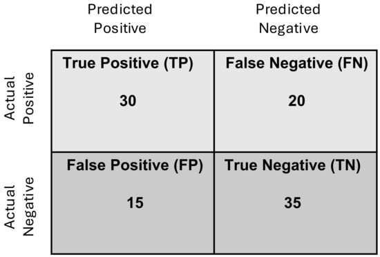
Figure 1.
Example confusion matrix for a hypothetical test set of 100 samples. Each cell in the matrix represents the count of samples corresponding to a specific classification outcome. The rows denote the actual class labels (True Positive or True Negative), while the columns represent the predicted class labels (positive or negative). For instance, the top-left cell indicates the number of True Positives (samples correctly classified as positive), while the bottom-right cell shows the number of True Negatives (samples correctly classified as negative). The off-diagonal cells represent classification errors: the top-right cell shows False Positives (samples incorrectly classified as positive), and the bottom-left cell indicates False Negatives (samples incorrectly classified as negative). Based on this confusion matrix, Accuracy = 0.65, Precision = 0.66, Sensitivity = 0.60, Specificity = 0.7.
From the confusion matrix, several performance metrics are derived. Of those, accuracy is the most intuitive one. Accuracy measures the ratio of correctly predicted instances to the total number of instances and is defined as
Precision (Positive Predictive Value) calculates the proportion of True Positive predictions among all positive predictions, expressed as
Sensitivity (Recall or True Positive Rate) measures the proportion of actual positive instances correctly identified by the model and is defined as
Specificity, also known as the True Negative Rate, measures the proportion of actual negative instances correctly identified by the model. It is defined as
Accuracy, while a commonly used metric, has a significant deficiency when applied to unbalanced datasets, as it can be misleading by favoring the majority class [52]. Other metrics, such as balanced accuracy and F1-Score, are often used to address such scenarios. Balanced Accuracy provides a more comprehensive evaluation of model performance on unbalanced datasets by averaging the sensitivity and specificity. It is defined as
This metric ensures that both the positive and negative classes are given equal importance, offering a more balanced view of the model’s performance, especially when class distributions are skewed.
The F1-Score, a harmonic mean of precision and recall, balances the trade-off between the two and is given by
Additionally, the false discovery rate (FDR), defined as
quantifies the proportion of False Positives among all positive predictions and is particularly valuable in high-dimensional datasets, such as those encountered in bioinformatics. This is critical in bioinformatics because high-dimensional data often involve multiple hypothesis testing, where controlling False Positives is essential to ensure the reliability of identified biomarkers or biological insights.
All the metrics discussed above rely on binary predictions from algorithms, which necessitates the definition of a decision threshold to convert the continuous confidence scores into binary predictions. However, there are alternative metrics that directly utilize the confidence scores provided by algorithms, such as the Area Under the Receiver Operating Characteristic Curve (AUROC) [53] and the Precision–Recall Area Under the Curve (PRAUC) [54]. These metrics evaluate the performance of models across a range of thresholds rather than relying on a fixed decision threshold. This approach offers several benefits, including a more comprehensive assessment of model performance, particularly in scenarios with unbalanced datasets or varying threshold requirements [55]. Of these metrics, to calculate the AUROC, one first needs to plot the Receiver Operating Characteristic (ROC) curve, which displays the True Positive Rate (sensitivity) against the False Positive Rate (specificity) across varying thresholds. The area under the ROC curve quantifies the AUROC metric. AUROC summarizes the model’s ability to distinguish between positive and negative classes. AUC ranges from 0.5 (random guessing) to 1.0 (perfect classification) and provides a single scalar value that captures the overall performance of the model across all thresholds. PRAUC, on the other hand, provides a single scalar value summarizing the model’s ability to balance precision and recall across a range of thresholds. PRAUC ranges between 0 and 1, where a PRAUC of 1.0 indicates perfect classification, with the model achieving both high precision and high recall at all thresholds. A lower PRAUC reflects weaker performance, and the PRAUC of a random classifier is the prevalence of the positive class. Unlike AUROC, which evaluates the model’s ability to distinguish between positive and negative classes, PRAUC focuses specifically on the performance of the positive class. This makes it particularly well suited for scenarios with imbalanced datasets, where the positive class is underrepresented, and traditional metrics like accuracy or AUROC may provide misleading assessments [56]. Table 1 provides a comparison of AUROC and PRAUC.

Table 1.
Comparison of AUROC and PRAUC metrics.
3. Reframing Bioinformatics Tasks as Binary Classification Challenges
In this section, we will demonstrate that a wide range of common bioinformatics tasks can be effectively reframed as binary classification problems, providing a structured and systematic approach to addressing these challenges. Furthermore, for many of these tasks, a variety of algorithms have been developed, each with unique strengths and limitations. This diversity of different algorithms makes these tasks particularly well suited for ensemble learning, where multiple algorithms can be combined to enhance predictive accuracy and generalizability.
3.1. Differential Expression Calling
Differential expression calling is a fundamental task in bioinformatics that involves identifying genes, transcripts, or other molecular features that exhibit significant changes in expression levels between two or more experimental conditions, such as treatment versus control or diseased versus healthy samples [57]. This analysis is critical for understanding the molecular mechanisms underlying biological processes and diseases, as well as for identifying potential biomarkers or therapeutic targets. Differential expression is typically determined by comparing the expression profiles of features across groups, often using statistical methods to test for significant differences. While differential expression analysis can be applied to both RNA-seq and microarray data, this discussion will focus on RNA-seq for illustrative purposes.
This task can be naturally cast as a binary classification problem. Each gene or molecular feature can be treated as a data point, represented by a feature vector of expression levels across samples. The goal is to classify each feature into one of two classes: “differentially expressed” (positive class) or “not differentially expressed” (negative class). This framing allows the application of algorithms to predict class membership based on the statistical or computational criteria derived from the data. DESeq2 is a widely used algorithm for differential expression analysis, designed to model RNA sequencing (RNA-seq) count data using a negative binomial distribution [58]. This model accounts for overdispersion in the data, where variance exceeds the mean, by estimating a dispersion parameter for each gene. DESeq2 generates a p-value which quantifies the likelihood that the observed difference in gene expression is due to random variation, with smaller p-values indicating potential differential expression. DESeq2 adjusts these p-values for multiple testing using methods like the Benjamini–Hochberg procedure, resulting in an adjusted p-value (FDR) that controls the false discovery rate. Genes can be classified as differentially expressed (belonging to the positive class) if their FDR falls below a significance threshold, such as 0.05. Another popular method for differential expression calling from RNA-seq is the limma-voom [25]. The algorithm first transforms count data into log2-counts per million (log-CPM) while estimating the mean–variance relationship, which is used to assign precision weights to each observation. This allows the use of linear modeling and empirical Bayes methods, originally developed for microarray data, to perform robust statistical testing. Similar to DESeq2, the method generates p-values for each gene by testing the null hypothesis that the gene’s expression is identical across conditions which can be used for differential expression calling across experimental conditions. In addition to the two widely used algorithms described above, there are several less popular but noteworthy tools for differential expression analysis. Examples include Cuffdiff [59], which uses a beta-negative binomial model to test for significant changes in transcript expression levels between conditions by accounting for variability in RNA-seq data and transcript assembly. baySeq adopts a Bayesian approach to estimate the posterior likelihood of differential expression, offering the robust handling of biological replicates and variability [60]. NOISeq employs a non-parametric method based on noise modeling to assess differential expression, making it particularly suitable for datasets with limited replicates or non-standard distributions [61]. Each of these algorithms offers unique methodologies tailored to different experimental conditions and data characteristics, expanding the toolkit for analyzing complex expression datasets. We emphasize that differential expression analysis is inherently an unsupervised learning problem, as it lacks labeled data for training, making it particularly well suited for unsupervised ensemble learning approaches.
3.2. Network Inference
Here, we will describe the network inference problem and how it can be cast as a binary classification problem. We will use gene regulatory networks for illustration purposes, but the methodology described is generic and can be readily applied to other networks, such as Protein–Protein Interaction Networks (PPINs), Signaling Networks, and Drug-Target Networks [62,63,64,65]. Gene regulatory networks (GRNs) model the regulatory relationships between genes, particularly how transcription factors (TFs) control the expression of target genes [66]. Mathematically, GRNs can be represented as a directed graph , where V represents genes (including transcription factors) and E represents regulatory interactions (edges) between them. Each edge indicates that gene i regulates gene j. The gene network inference task involves predicting whether a regulatory edge exists between a pair of genes based on experimental data, such as gene expression profiles. This task can be cast as a binary classification problem, where the objective is to learn a function, mapping features derived from the data to a binary label: 1 if an edge exists (regulation), and 0 otherwise (no regulation).
One of the most popular algorithms for GRN inference is the WGCNA algorithm [28]. WGCNA constructs gene co-expression networks by identifying modules of genes with highly correlated expression patterns. It begins by calculating the pairwise correlation matrix , where each entry represents the correlation between the expression profiles of genes i and j, denoted as and . This matrix is then transformed into a weighted adjacency matrix using a power adjacency function, , where is a soft-thresholding parameter that ensures the resulting network adheres to a scale-free topology, commonly observed in biological systems [67]. The algorithm then computes the Topological Overlap Matrix (TOM), which measures the similarity between genes based on their shared connections within the network (for details, see [28]). Hierarchical clustering of the TOM-based dissimilarity metric identifies gene modules, which, along with their hub genes, can be correlated with external traits to uncover biologically relevant patterns and regulatory insights.
One of the drawbacks of the WGCNA algorithm is its sensitivity to linear relationships, as it primarily relies on the pairwise correlation matrix , where each entry represents the Pearson (or another type of) correlation between genes i and j. This reliance on correlation means that WGCNA may have a lower sensitivity to detect nonlinear dependencies between gene expression profiles, which are common in biological systems. To address this limitation, the ARACNE (Algorithm for the Reconstruction of Accurate Cellular Networks) algorithm was introduced [27]. ARACNE focuses on capturing nonlinear relationships by leveraging mutual information (MI) instead of correlation. Mutual information quantifies the dependency between two random variables, capturing both linear and nonlinear interactions [68]. For two genes i and j, the mutual information is defined as
where is the joint probability density function of the expression levels of i and j, and and are their marginal probability density functions.
ARACNE constructs a network adjacency matrix , where each entry represents the mutual information between genes i and j:
where is a threshold for filtering insignificant interactions. To further refine the network, ARACNE applies the Data Processing Inequality (DPI), which removes indirect interactions by considering the triplet . If the mutual information between two genes is mediated by a third gene (e.g., ), the weaker interaction () is removed.
Although WGCNA and ARACNE are among the most popular network inference algorithms, several other methods have been proposed for GRN inference, utilizing diverse approaches. GENIE3 uses random forests to model the expression of target genes as a function of transcription factors, ranking interactions based on feature importance [69]. TIGRESS combines LASSO regression with stability selection to identify robust regulatory relationships, ensuring reliability across multiple data subsamples [70]. Bayesian methods like BANJO and GRENITS model GRNs as directed acyclic graphs (DAGs), capturing conditional dependencies and assigning probabilistic scores to interactions [71,72]. The PHIXER algorithm employs an information-theoretic quantity called the phi-mixing coefficient, which measures the statistical dependence between variables, to infer regulatory interactions while accounting for nonlinearity and noise [73]. We would like to emphasize that all the above methodologies use unlabeled data to infer GRNs. Hence, similar to differential expression calling, these diverse methodologies highlight the complementary strengths of different approaches, underscoring the potential for unsupervised ensemble learning to integrate these methods and achieve more robust and accurate inference of complex regulatory networks.
3.3. Somatic Mutation Calling
Somatic mutation calling is a key task in bioinformatics aimed at identifying genetic mutations that occur in somatic cells, typically in the context of diseases such as cancer. Unlike germline mutations, which are inherited and present in all cells of an organism, somatic mutations arise spontaneously and are confined to specific tissues or cell types. Detecting somatic mutations is crucial for understanding tumor evolution, identifying driver mutations, and informing precision medicine approaches [74].
Mathematically, somatic mutation calling involves distinguishing between true somatic mutations and sequencing or mapping errors in a given set of DNA sequencing data. Each position in the genome can be represented by a feature vector , where and represent the read counts supporting the reference allele in normal and tumor samples, respectively, and and represent the counts supporting the alternate allele. The binary classification task is then to assign a class label to each genomic position i: somatic mutation (positive class) or no mutation (negative class).
Statistical models such as the binomial distribution are commonly employed in mutation calling algorithms [75]. For example, the likelihood of observing the alternate allele in the tumor sample can be modeled as
where is the total number of reads in the tumor sample, is the number of reads supporting the alternate allele, and is the expected frequency of the alternate allele based on normal samples.
Algorithms such as Mutect2 use probabilistic frameworks to compare allele frequencies in tumor and matched normal samples, leveraging a likelihood ratio test to distinguish somatic mutations from germline variants and sequencing artifacts [76]. For a given genomic position, the likelihood ratio is defined as
A position is classified as a somatic mutation if exceeds a predefined threshold, adjusted for multiple testing using methods like the Benjamini–Hochberg procedure to control the false discovery rate. Thus, this quantity can serve as a scoring function. Mutect2 further integrates statistical filtering for strand bias, contamination, and mapping artifacts, improving its performance in low-purity or low-depth samples.
Other widely used algorithms include Strelka and VarScan, which extend these probabilistic frameworks with additional features and statistical filters [77,78]. Strelka uses a Bayesian model to simultaneously call germline and somatic variants, incorporating tumor purity estimates to improve sensitivity in heterogeneous samples [77]. VarScan, on the other hand, applies heuristic filters for allele frequency thresholds and strand bias, making it efficient and straightforward for targeted sequencing datasets [78].
3.4. Other Common Bioinformatics Tasks as Binary Classification Problems
In addition to differential expression calling, network inference, and somatic mutation calling, a wide array of bioinformatics tasks can be effectively framed as binary classification problems. Due to space constraints, we will only describe them briefly in this section. One such task is variant calling, which involves identifying germline mutations from sequencing data [79]. The goal is to classify whether a variant is present or absent at each genomic position. Variant calling typically uses whole-genome sequencing (WGS) or whole-exome sequencing (WES) data, where high-quality read alignments are essential to ensure accurate classification. Algorithms like the GATK HaplotypeCaller and FreeBayes apply probabilistic models to assign likelihood scores based on these features, which are then thresholded to make binary decisions [80,81].
Similarly, biomarker discovery aims to classify molecular features, such as genes, proteins, or metabolites, as relevant (biomarkers) or irrelevant. This task combines statistical methods with machine learning techniques to identify robust biomarkers from high-dimensional datasets, such as transcriptomics, proteomics, or metabolomics data [82]. Another common task is protein function prediction, where the goal is to classify whether a given protein belongs to a specific functional category, such as “enzyme” or “non-enzyme” [83]. Features such as sequence similarity, structural properties, and evolutionary information are used as inputs for algorithms. Likewise, epigenetic state classification involves determining whether a genomic region exhibits a specific epigenetic state, such as methylation or chromatin accessibility [84]. Sequencing data like ChIP-seq, ATAC-seq, or methylation arrays are commonly utilized to train predictive models [85,86].
Gene essentiality prediction is yet another example where genes are classified as essential or non-essential for cellular survival [87]. CRISPR-Cas9 screening data or RNAi datasets provide the basis for training machine learning models for this task. In [87], the authors give an extensive comparison of various machine learning models for this task. In metabolic pathway identification, the objective is to classify whether specific metabolites belong to a particular pathway, using features derived from metabolomic data, reaction databases, and pathway annotations (a review of different machine learning models for this task is given in [88]).
Clinical outcome prediction is another crucial task in translational bioinformatics. This involves classifying whether a patient will respond to a specific therapy or whether a treatment will lead to adverse effects. Predictive models for such tasks integrate genetic, transcriptomic, and clinical data, providing valuable insights for personalized medicine [89].
In addition to the tasks described, there are numerous other bioinformatics challenges that can be framed as binary classification problems. Examples include identifying enhancer regions [90], detecting alternative splicing events [91], or predicting the pathogenicity of genetic variants [92]. Beyond these, there are many other tasks not discussed here, as our goal is to provide a representative overview rather than an exhaustive list. By highlighting key examples, we aim to illustrate the versatility of the binary classification framework in addressing diverse bioinformatics problems. Moreover, for each of these tasks, several algorithms have been proposed, each with unique strengths and assumptions, enabling the use of ensemble learning to enhance performance. Finally, although some of the above tasks, such as protein function prediction, can be considered semi-supervised since known protein functions can be used to train models, most of these problems are inherently unsupervised due to the absence of labeled data. This makes them particularly well suited for unsupervised ensemble learning approaches, which can effectively integrate and leverage predictions from multiple algorithms without the need for labels. In the next section, we will give an overview of ensemble learning with a specific focus on unsupervised ensemble learning.
4. Introduction to Ensemble Learning
Ensemble learning is a machine learning approach that aggregates the outputs of multiple models to improve predictive performance, reduce errors, and increase robustness [93]. Formally, let represent M individual models, each designed to approximate a binary outcome for binary classification. The models in an ensemble can be constructed using the same dataset with shared features, or they can originate from entirely different datasets that may not share features. Moreover, the models within an ensemble can employ distinct modeling strategies, such as using different types of algorithms.
Diversity among the models is a critical factor in enhancing the effectiveness of an ensemble [94]. In cases where the models use the same training dataset, diversity can be introduced by resampling techniques, such as bootstrapping, or by using different modeling methodologies [95]. On the other hand, when the models are derived from different datasets, the absence of shared features can inherently contribute to diversity, as each model learns from distinct patterns or distributions. Additionally, using different algorithms introduces methodological diversity, as each algorithm brings unique assumptions, learning strategies, and biases that can complement one another in ensemble predictions.
Ensemble learning methods can be broadly categorized into two main types: supervised ensemble learning and unsupervised ensemble learning. Supervised ensemble algorithms, in turn, can be further divided into two subcategories, homogeneous ensembles [96,97] and heterogeneous ensembles [98], based on the nature of the individual models used in the ensemble. Homogeneous ensembles consist of models of the same type, such as decision trees in random forests or gradient boosting [99]. These models typically differ in their training data, parameters, or initialization, creating diversity despite their shared architecture. Techniques like bagging (e.g., random forests) introduce diversity by training each model on a different subset of the data, while boosting methods (e.g., AdaBoost and XGBoost) iteratively adjust the training process to focus on previously misclassified instances [100]. In contrast, heterogeneous ensembles combine models of different types, such as neural networks, support vector machines, and decision trees [94]. This approach leverages the unique strengths and capabilities of each model type, enabling the ensemble to capture a wider variety of patterns and relationships in the data. Heterogeneous ensembles are particularly effective for handling complex and noisy datasets, such as those commonly encountered in biology, where the assumptions underlying individual algorithms may not hold consistently across the data. Biological datasets, such as those derived from genomics, transcriptomics, or proteomics, are often high-dimensional, sparse, and affected by measurement noise or batch effects. In such scenarios, relying on a single algorithm may lead to suboptimal performance, as different algorithms are sensitive to specific data characteristics or assumptions, such as linearity, independence, or distributional properties. By combining models of different types, heterogeneous ensembles integrate diverse perspectives, leveraging the unique strengths of each algorithm.
Although supervised ensembles can be effectively applied to certain biological problems that have labeled datasets, such as disease classification, gene essentiality prediction, and drug response prediction, many biological tasks are inherently unlabeled. Examples of these tasks include differential expression calling, somatic mutation detection, and network inference, where the true class labels (e.g., differentially expressed vs. non-differentially expressed genes, or interacting vs. non-interacting genes) are typically unknown or scarce. In such cases, unsupervised ensemble methods are most appropriate.
Before delving into unsupervised ensemble learning methods, it is important to first examine the general disadvantages of unsupervised learning and the critical role ensemble methods play in addressing these challenges. Unsupervised machine learning faces several limitations, many of which can be mitigated through ensemble approaches [101]. One major issue is the lack of ground truth, which makes it difficult to evaluate the quality of patterns or clusters. Ensemble methods tackle this by combining predictions from multiple models, enhancing robustness and reducing bias [102]. Additionally, unsupervised models are sensitive to noise, which can obscure the true structure of the data. Techniques like bagging or boosting help counter this by averaging results across models, thereby minimizing the impact of noise [103]. Lastly, overfitting is a concern, particularly with complex models or arbitrary parameter choices, but ensemble techniques mitigate this by averaging predictions, reducing variance, and improving generalization. Through these mechanisms, ensemble methods significantly enhance the effectiveness and reliability of unsupervised learning.
The simplest unsupervised ensemble algorithm creates an ensemble score by calculating the unweighted average of the predictions made by the base classifiers for each item being classified [41]. Formally, let represent the prediction score assigned to item j by classifier i, where and . The ensemble prediction score for item j is then given by:
This approach assumes that all base classifiers contribute equally to the final decision. Known as the “Wisdom of Crowds” (WOC) method (Surowiecki, 2005), it is simple and computationally efficient but performs poorly when a majority of base classifiers generate unreliable predictions since it assigns equal importance to each algorithm.
For the case where algorithms provide binary predictions, an early approach that improved on the WOC approach was introduced by Dawid and Skene (1979), who proposed a model that jointly infers both the true class labels and the performance of each classifier. Let represent the predictions of classifier i, where is the predicted label for item j. The Dawid–Skene model assumes a conditional independence structure and models the likelihood of observed predictions as
where parameterizes the performance of each classifier. Using the Expectation–Maximization (EM) algorithm [104], the model estimates and simultaneously. While this method is elegant, it faces limitations due to the non-convex optimization challenges of the EM algorithm. The SML algorithm, introduced in [105], improves upon the Dawid and Skene model by providing a computationally efficient and asymptotically consistent solution to the problem of inferring true labels and classifier accuracies. Unlike Dawid and Skene’s reliance on non-convex iterative likelihood maximization, which is prone to local optima and computational inefficiency, SML leverages the observation that, under standard independence assumptions, the off-diagonal elements of the classifiers’ covariance matrix form a rank-one matrix. The eigenvector of this matrix contains entries proportional to the classifiers’ balanced accuracies (which is defined as the average of the sensitivity and specificity of the algorithm), allowing for direct and efficient computation of classifier weights. This novel approach avoids the iterative nature of traditional methods, making SML more robust, scalable, and practical for high-dimensional, noisy datasets commonly encountered in real-world applications.
Although SML is an improvement on the Dawid and Skene method, both methods assume binary predictions by algorithms, and do not work with algorithms providing continuous confidence scores, which is very common in bioinformatics tasks. This leads to suboptimal performance in cases with rank-based or confidence-weighted predictions, which is usually the case in bioinformatics algorithms. In general, many bioinformatics algorithms produce continuous scores, such as p-values, which often need to be converted into binary predictions. This is typically achieved by applying a not-always well-calibrated threshold, a process that can lead to suboptimal performance due to the loss of information inherent in the continuous scores and the potential misclassification caused by poorly chosen thresholds. These drawbacks underscore the need for unsupervised approaches that can use the continuous scores provided by individual algorithms. A significant challenge in bioinformatics with algorithms providing continuous prediction scores, however, is the variability in the scales of predictions generated by different algorithms, which can complicate their integration and comparison. For example, in network inference, ARACNe produces network weights based on mutual information, a measure without a fixed range, while WGCNA generates correlations as network weights that are constrained to a range between [0, 1]. These differences in scale and interpretation of outputs make it difficult to directly compare or combine predictions from these algorithms, potentially leading to inconsistent or biased results when integrating outputs in downstream analyses. To address both challenges, the Strategy for Unsupervised Multiple Method Aggregation (SUMMA) was introduced in [43]. SUMMA employs a preprocessing step that converts continuous predictions into a matrix of ranked predictions. This approach standardizes the output from diverse classifiers by replacing raw confidence scores with ranks, ensuring comparability across methods. For each base classifier, the predictions are ranked in descending order, with the highest confidence score assigned the top rank. This rank transformation not only mitigates the issue of differing scales but also reduces the impact of outliers or extreme values in the continuous predictions, which might otherwise skew the aggregation process. Similar to SML, SUMMA is an unsupervised ensemble approach and assumes conditional independence between predictions but utilizes the covariance matrix of ranked predictions to estimate each classifier’s performance in terms of AUC. By integrating these performance estimates into a maximum likelihood framework, SUMMA produces a robust ensemble classifier that is not only unsupervised but also capable of assigning weights to classifiers proportional to their inferred accuracy. Recent advancements further extended the ensemble learning paradigm through FiDEL (Fermi–Dirac-based Ensemble Learning), which leverages statistical physics principles [106]. FiDEL employs the Fermi–Dirac (FD) distribution to provide calibrated probabilistic outputs, mapping the rank-conditioned probabilities of classifier outputs to the behavior of fermions in quantum systems. This approach optimally combines ranks from multiple classifiers while accounting for their relative accuracies. The reliance of FiDEL on the FD distribution ensures an unbiased probabilistic representation of classifier ranks, offering robust generalization even when conditional independence assumptions are mildly violated. In a similar vein, the MOCA framework offers two ensemble strategies: unsupervised MOCA (uMOCA) and supervised MOCA (sMOCA) [93]. uMOCA is designed for scenarios without labeled data, where classifier weights are estimated based on the rank transformation of classifier predictions and their second- and third-order statistical moments. This enables optimal weight assignment under the assumption of class-conditioned independence, allowing the aggregation of diverse classifier outputs without overfitting. On the other hand, sMOCA leverages labeled data to compute class-conditioned means and covariance matrices, enabling it to address dependencies between classifiers by incorporating correlation structures.
In addition, recent advances in deep learning have introduced novel approaches to unsupervised ensemble learning. One notable contribution is the development of a Restricted Boltzmann Machine (RBM)-based Deep Neural Network (DNN) model for addressing challenges where the assumption of conditional independence among classifiers is violated [107]. This approach leverages the equivalence of the Dawid–Skene (DS) model to an RBM with a single hidden node, allowing posterior probabilities of true labels to be estimated effectively. Furthermore, the RBM-based DNN extends beyond the DS model by incorporating multiple layers of hidden units, enabling it to capture and disentangle dependencies among classifiers. This is particularly important because the previously introduced algorithms rely on the assumption of conditional independence between classifiers. However, in practice, most bioinformatics algorithms violate this assumption due to overlapping features, shared preprocessing steps, or shared training data, which introduce correlations between classifier outputs. Figure 2 illustrates the workflow of unsupervised learning, using network inference as an example task.
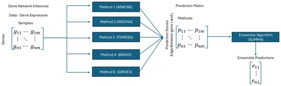
Figure 2.
An example figure illustrating unsupervised learning in bioinformatics. The figure demonstrates unsupervised learning using GRN inference as an example where we want to predict whether genes i and j interact.
In many bioinformatics tasks, such as differential expression analysis and somatic mutation detection, the lack of labeled data necessitates the use of unsupervised ensemble learning approaches. However, for certain tasks like gene or protein function prediction, a different machine learning paradigm, semi-supervised learning, can be utilized [108]. Semi-supervised learning is particularly suitable for tasks where a small subset of the data is annotated with high-confidence labels (gold standard) while the majority remains unlabeled. For instance, in gene function prediction, some genes have experimentally verified functions (labeled data), whereas the vast majority of genes remain uncharacterized (unlabeled data). The scarcity of labeled data and the high cost of experimental validation make gene function prediction an ideal candidate for semi-supervised learning. Semi-supervised learning is a machine learning paradigm that combines the strengths of supervised and unsupervised learning by leveraging both labeled and unlabeled data [109]. In many real-world scenarios, acquiring labeled data can be expensive, time-consuming, or impractical, while unlabeled data are often abundant and easy to collect. Semi-supervised learning addresses this imbalance by using a small set of labeled data to guide the learning process and a larger set of unlabeled data to uncover patterns and structure in the data distribution [110]. A key advantage of semi-supervised learning is its ability to enhance generalization by effectively utilizing the information present in unlabeled data. Common techniques in semi-supervised learning include self-training, co-training, and graph-based methods. In self-training, the model iteratively labels the unlabeled data using its predictions, which are then incorporated into the training process [111]. Co-training employs multiple learners that label data for one another, improving robustness and reducing bias [112]. Graph-based approaches leverage the relationships between data points to propagate labels through the dataset [113].
These advancements underscore the growing importance of developing ensemble learning methods that can adapt to the dependencies and complexities inherent in real-world bioinformatics tasks. Researchers can achieve more accurate and robust predictions by integrating approaches like SUMMA, which effectively addresses the challenges of varying prediction scales and unlabeled data, with RBM-based DNNs that handle classifier dependencies. By combining insights and predictions from multiple algorithms, ensemble methods can mitigate the biases and limitations of individual models, leading to results that are not only more accurate but also more interpretable. Finally, although out of the scope of the current manuscript, several important supervised ensemble learning algorithms, such as negative correlation-based deep ensemble methods, can be useful in certain bioinformatics tasks, such as disease outcome prediction and drug response prediction. A thorough review of supervised ensemble learning methods can be found in [114]. Finally, we summarize and compare the three types of ensemble learning in Table 2.
Table 2.
A brief comparison of supervised, unsupervised, and semi-supervised ensemble learning.
5. Discussion and Conclusions
The complexities and heterogeneity of biomedical data present unique challenges, particularly when selecting optimal algorithms for various bioinformatics tasks. This variability stems from differences in data distributions, noise levels, and the underlying biological contexts. Traditional single-method approaches often fail to generalize across diverse datasets, emphasizing the need for robust methodologies that can integrate insights from multiple algorithms. Ensemble learning has emerged as a powerful solution, leveraging the strengths of diverse algorithms to provide more reliable and accurate results.
Unsupervised ensemble learning, in particular, holds immense promise for addressing challenges in bioinformatics, where labeled data are often scarce or unavailable. By aggregating predictions from multiple methods, unsupervised ensembles provide a way to combine the strengths of individual algorithms while mitigating their weaknesses. While ensemble learning has demonstrated significant potential and has been successfully applied to specific bioinformatics tasks such as gene network inference and protein function prediction, our review of the literature suggests that its adoption remains less common in other areas of bioinformatics, such as differential expression analysis and mutation calling.
However, there are still limitations that need to be addressed. Many current unsupervised ensemble approaches assume conditional independence among classifiers, an assumption that may not always hold in real-world applications where classifiers often share overlapping features or data preprocessing steps. Violations of this assumption can lead to biased results and suboptimal performance. Future research can tackle this limitation by assuming some structure of dependence between algorithms in the case of the absence of labels. If there are limited labeled data, another promising future direction is the exploration of methods to effectively utilize limited labeled data for estimating the conditional correlation between classifiers. Missing data, a prevalent challenge in bioinformatics, can significantly undermine the reliability of ensemble methods by disrupting both prediction aggregation and the accurate estimation of classifier performance. For example, in tasks such as gene expression analysis, missing values in high-dimensional datasets can lead to biased results when aggregating predictions across classifiers. Similarly, in protein structure prediction, incomplete feature sets might affect the performance of individual models, skewing the overall ensemble output. To address these challenges, future developments in ensemble learning should focus on incorporating mechanisms such as imputation strategies tailored to ensemble models, robust aggregation techniques that can handle missing predictions, and ensemble frameworks designed to adaptively weight classifiers based on the completeness of their input data. Another promising direction is the development of adaptive ensemble methods that dynamically adjust weights or model contributions based on data characteristics or intermediate results, allowing for more robust and context-sensitive performance. For example, ensembles could be designed to identify and mitigate poorly performing models, enhancing overall effectiveness. Additionally, explainability frameworks for unsupervised ensembles can foster trust and usability by providing transparent insights into the contributions of individual models, particularly in sensitive domains like bioinformatics and healthcare. To enhance explainability in unsupervised ensemble learning, several strategies can be employed. One approach is to develop methods that quantify and visualize the contribution of each model in the ensemble to the final output, using techniques like Shapley values or feature importance rankings to highlight individual model influences. Designing tools to trace how intermediate outputs from individual models combine to form the final decision, such as graph-based consensus representations, can also improve transparency. Also, the design of benchmark datasets and evaluation metrics tailored to unsupervised ensemble methods is another critical area, as standardized tools can enable consistent performance assessment and comparison across studies. Finally, theoretical research to explore trade-offs between ensemble size, diversity, and stability can provide fundamental insights to guide the development of next-generation ensemble learning systems. Addressing these areas offers a pathway to significant advancements in both the theory and application of unsupervised ensemble learning.
In conclusion, as the field of bioinformatics continues to evolve, unsupervised ensemble learning offers a pathway to more robust and interpretable solutions, driving advancements in understanding biological systems and translating these insights into meaningful biomedical applications. By continuing to refine and innovate these methods, researchers can unlock new opportunities for addressing the challenges posed by the complexity and heterogeneity of biomedical data.
Funding
This research received no external funding.
Data Availability Statement
Data are contained within the article.
Conflicts of Interest
The author declares no conflicts of interest.
References
- Petrik, J. Microarray technology: The future of blood testing? Vox Sang. 2001, 80, 1–11. [Google Scholar] [CrossRef] [PubMed]
- Wang, J.H.; Liu, C.Y.; Min, Y.R.; Wu, Z.H.; Hou, P.L. Cancer diagnosis by gene-environment interactions via combination of SMOTE-Tomek and overlapped group screening approaches with application to imbalanced TCGA clinical and genomic data. Mathematics 2024, 12, 2209. [Google Scholar] [CrossRef]
- Heller, M.J. DNA microarray technology: Devices, systems, and applications. Annu. Rev. Biomed. Eng. 2002, 4, 129–153. [Google Scholar] [CrossRef] [PubMed]
- Müller, U.R.; Nicolau, D.V. Microarray Technology and Its Applications; Springer: Berlin/Heidelberg, Germany, 2005. [Google Scholar]
- Miller, M.B.; Tang, Y.W. Basic concepts of microarrays and potential applications in clinical microbiology. Clin. Microbiol. Rev. 2009, 22, 611–633. [Google Scholar] [CrossRef]
- Veiga, D.F.; Dutta, B.; Balázsi, G. Network inference and network response identification: Moving genome-scale data to the next level of biological discovery. Mol. BioSyst. 2010, 6, 469–480. [Google Scholar] [CrossRef]
- Madhamshettiwar, P.B.; Maetschke, S.R.; Davis, M.J.; Reverter, A.; Ragan, M.A. Gene regulatory network inference: Evaluation and application to ovarian cancer allows the prioritization of drug targets. Genome Med. 2012, 4, 41. [Google Scholar] [CrossRef]
- Ozsolak, F.; Milos, P.M. RNA sequencing: Advances, challenges and opportunities. Nat. Rev. Genet. 2011, 12, 87–98. [Google Scholar] [CrossRef]
- Zhang, W.; Yu, Y.; Hertwig, F.; Thierry-Mieg, J.; Zhang, W.; Thierry-Mieg, D.; Wang, J.; Furlanello, C.; Devanarayan, V.; Cheng, J.; et al. Comparison of RNA-seq and microarray-based models for clinical endpoint prediction. Genome Biol. 2015, 16, 133. [Google Scholar] [CrossRef]
- Kolodziejczyk, A.A.; Kim, J.K.; Svensson, V.; Marioni, J.C.; Teichmann, S.A. The technology and biology of single-cell RNA sequencing. Mol. Cell 2015, 58, 610–620. [Google Scholar] [CrossRef]
- Huang, Q.; Liu, Y.; Du, Y.; Garmire, L.X. Evaluation of cell type annotation R packages on single-cell RNA-seq data. Genom. Proteom. Bioinform. 2021, 19, 267–281. [Google Scholar] [CrossRef]
- Peng, J.; Sun, B.F.; Chen, C.Y.; Zhou, J.Y.; Chen, Y.S.; Chen, H.; Liu, L.; Huang, D.; Jiang, J.; Cui, G.S.; et al. Single-cell RNA-seq highlights intra-tumoral heterogeneity and malignant progression in pancreatic ductal adenocarcinoma. Cell Res. 2019, 29, 725–738. [Google Scholar] [CrossRef] [PubMed]
- Ding, S.; Chen, X.; Shen, K. Single-cell RNA sequencing in breast cancer: Understanding tumor heterogeneity and paving roads to individualized therapy. Cancer Commun. 2020, 40, 329–344. [Google Scholar] [CrossRef] [PubMed]
- Lee, J.; Kuo, Y.F.; Goodwin, J.S. The effect of electronic medical record adoption on outcomes in US hospitals. BMC Health Serv. Res. 2013, 13, 39. [Google Scholar] [CrossRef] [PubMed]
- Graber, M.L.; Byrne, C.; Johnston, D. The impact of electronic health records on diagnosis. Diagnosis 2017, 4, 211–223. [Google Scholar] [CrossRef]
- El-Kareh, R.; Hasan, O.; Schiff, G.D. Use of health information technology to reduce diagnostic errors. BMJ Qual. Saf. 2013, 22, ii40–ii51. [Google Scholar] [CrossRef]
- Tierney, M.J.; Pageler, N.M.; Kahana, M.; Pantaleoni, J.L.; Longhurst, C.A. Medical education in the electronic medical record (EMR) era: Benefits, challenges, and future directions. Acad. Med. 2013, 88, 748–752. [Google Scholar] [CrossRef]
- Ong, J.C.L.; Chen, M.; Ng, N.; Elangovan, K.; Tan, N.Y.T.; Jin, L.; Xie, Q.; Ting, D.S.W.; Rodriguez-Monguio, R.; Bates, D.; et al. Generative AI and Large Language Models in Reducing Medication Related Harm and Adverse Drug Events-A Scoping Review. medRxiv 2024. [Google Scholar] [CrossRef]
- Yin, H.; Tang, J.; Li, S.; Wang, T. LLMADR: A Novel Method for Adverse Drug Reaction Extraction Based on Style Aligned Large Language Models Fine-Tuning. In Proceedings of the CCF International Conference on Natural Language Processing and Chinese Computing, Hangzhou, China, 1–3 November 2024; Springer: Berlin/Heidelberg, Germany, 2024; pp. 470–482. [Google Scholar]
- Lahlou, C.; Crayton, A.; Trier, C.; Willett, E. Explainable health risk predictor with transformer-based medicare claim encoder. arXiv 2021, arXiv:2105.09428. [Google Scholar]
- Lee, S.A.; Lindsey, T. Do Large Language Models understand Medical Codes? arXiv 2024, arXiv:2403.10822. [Google Scholar]
- Baxevanis, A.D.; Bader, G.D.; Wishart, D.S. Bioinformatics; John Wiley & Sons: Hoboken, NJ, USA, 2020. [Google Scholar]
- Kalia, M. Biomarkers for personalized oncology: Recent advances and future challenges. Metabolism 2015, 64, S16–S21. [Google Scholar] [CrossRef]
- Li, Y.; Huang, C.; Ding, L.; Li, Z.; Pan, Y.; Gao, X. Deep learning in bioinformatics: Introduction, application, and perspective in the big data era. Methods 2019, 166, 4–21. [Google Scholar] [CrossRef] [PubMed]
- Law, C.W.; Chen, Y.; Shi, W.; Smyth, G.K. voom: Precision weights unlock linear model analysis tools for RNA-seq read counts. Genome Biol. 2014, 15, R29. [Google Scholar] [CrossRef] [PubMed]
- Love, M.; Anders, S.; Huber, W. Differential analysis of count data–the DESeq2 package. Genome Biol. 2014, 15, 550. [Google Scholar]
- Margolin, A.A.; Nemenman, I.; Basso, K.; Wiggins, C.; Stolovitzky, G.; Favera, R.D.; Califano, A. ARACNE: An algorithm for the reconstruction of gene regulatory networks in a mammalian cellular context. BMC Bioinform. 2006, 7, S7. [Google Scholar] [CrossRef]
- Langfelder, P.; Horvath, S. WGCNA: An R package for weighted correlation network analysis. BMC Bioinform. 2008, 9, 559. [Google Scholar] [CrossRef]
- Statnikov, A.; Aliferis, C.F.; Tsamardinos, I.; Hardin, D.; Levy, S. A comprehensive evaluation of multicategory classification methods for microarray gene expression cancer diagnosis. Bioinformatics 2005, 21, 631–643. [Google Scholar] [CrossRef]
- Ng, S.; Masarone, S.; Watson, D.; Barnes, M.R. The benefits and pitfalls of machine learning for biomarker discovery. Cell Tissue Res. 2023, 394, 17–31. [Google Scholar] [CrossRef]
- Litjens, G.; Kooi, T.; Bejnordi, B.E.; Setio, A.A.A.; Ciompi, F.; Ghafoorian, M.; Van Der Laak, J.A.; Van Ginneken, B.; Sánchez, C.I. A survey on deep learning in medical image analysis. Med. Image Anal. 2017, 42, 60–88. [Google Scholar] [CrossRef]
- Lundervold, A.S.; Lundervold, A. An overview of deep learning in medical imaging focusing on MRI. Z. Für Med. Phys. 2019, 29, 102–127. [Google Scholar] [CrossRef]
- Chibyshev, T.; Krasnova, O.; Chabina, A.; Gursky, V.V.; Neganova, I.; Kozlov, K. Image Processing Application for Pluripotent Stem Cell Colony Migration Quantification. Mathematics 2024, 12, 3584. [Google Scholar] [CrossRef]
- Rai, H.M.; Dashkevych, S.; Yoo, J. Next-Generation Diagnostics: The Impact of Synthetic Data Generation on the Detection of Breast Cancer from Ultrasound Imaging. Mathematics 2024, 12, 2808. [Google Scholar] [CrossRef]
- Si, Y.; Du, J.; Li, Z.; Jiang, X.; Miller, T.; Wang, F.; Zheng, W.J.; Roberts, K. Deep representation learning of patient data from Electronic Health Records (EHR): A systematic review. J. Biomed. Inform. 2021, 115, 103671. [Google Scholar] [CrossRef]
- Lin, C.; Zhang, Y.; Ivy, J.; Capan, M.; Arnold, R.; Huddleston, J.M.; Chi, M. Early diagnosis and prediction of sepsis shock by combining static and dynamic information using convolutional-LSTM. In Proceedings of the 2018 IEEE International Conference on Healthcare Informatics (ICHI), New York, NY, USA, 4–7 June 2018; IEEE: Piscataway, NJ, USA, 2018; pp. 219–228. [Google Scholar]
- Urbanowicz, R.J.; Olson, R.S.; Schmitt, P.; Meeker, M.; Moore, J.H. Benchmarking relief-based feature selection methods for bioinformatics data mining. J. Biomed. Inform. 2018, 85, 168–188. [Google Scholar] [CrossRef] [PubMed]
- Marbach, D.; Prill, R.J.; Schaffter, T.; Mattiussi, C.; Floreano, D.; Stolovitzky, G. Revealing strengths and weaknesses of methods for gene network inference. Proc. Natl. Acad. Sci. USA 2010, 107, 6286–6291. [Google Scholar] [CrossRef] [PubMed]
- Li, Y.; Ge, X.; Peng, F.; Li, W.; Li, J.J. Exaggerated false positives by popular differential expression methods when analyzing human population samples. Genome Biol. 2022, 23, 79. [Google Scholar] [CrossRef] [PubMed]
- Soneson, C.; Delorenzi, M. A comparison of methods for differential expression analysis of RNA-seq data. BMC Bioinform. 2013, 14, 91. [Google Scholar] [CrossRef]
- Marbach, D.; Costello, J.C.; Küffner, R.; Vega, N.M.; Prill, R.J.; Camacho, D.M.; Allison, K.R.; Kellis, M.; Collins, J.J.; Stolovitzky, G. Wisdom of crowds for robust gene network inference. Nat. Methods 2012, 9, 796–804. [Google Scholar] [CrossRef]
- Xu, H.; DiCarlo, J.; Satya, R.V.; Peng, Q.; Wang, Y. Comparison of somatic mutation calling methods in amplicon and whole exome sequence data. BMC Genom. 2014, 15, 244. [Google Scholar] [CrossRef]
- Ahsen, M.E.; Vogel, R.M.; Stolovitzky, G.A. Unsupervised evaluation and weighted aggregation of ranked classification predictions. J. Mach. Learn. Res. 2019, 20, 1–40. [Google Scholar]
- Mienye, I.D.; Sun, Y. A survey of ensemble learning: Concepts, algorithms, applications, and prospects. IEEE Access 2022, 10, 99129–99149. [Google Scholar] [CrossRef]
- Choobdar, S.; Ahsen, M.E.; Crawford, J.; Tomasoni, M.; Fang, T.; Lamparter, D.; Lin, J.; Hescott, B.; Hu, X.; Mercer, J.; et al. Assessment of network module identification across complex diseases. Nat. Methods 2019, 16, 843–852. [Google Scholar] [CrossRef] [PubMed]
- Schaffter, T.; Buist, D.S.; Lee, C.I.; Nikulin, Y.; Ribli, D.; Guan, Y.; Lotter, W.; Jie, Z.; Du, H.; Wang, S.; et al. Evaluation of combined artificial intelligence and radiologist assessment to interpret screening mammograms. JAMA Netw. Open 2020, 3, e200265. [Google Scholar] [CrossRef] [PubMed]
- Menden, M.P.; Wang, D.; Guan, Y.; Mason, M.J.; Szalai, B.; Bulusu, K.C.; Yu, T.; Kang, J.; Jeon, M.; Wolfinger, R.; et al. A cancer pharmacogenomic screen powering crowd-sourced advancement of drug combination prediction. BioRxiv 2017, 200451. [Google Scholar] [CrossRef]
- Tanevski, J.; Nguyen, T.; Truong, B.; Karaiskos, N.; Ahsen, M.E.; Zhang, X.; Shu, C.; Xu, K.; Liang, X.; Hu, Y.; et al. Gene selection for optimal prediction of cell position in tissues from single-cell transcriptomics data. Life Sci. Alliance 2020, 3, e202000867. [Google Scholar] [CrossRef]
- Alloghani, M.; Al-Jumeily, D.; Mustafina, J.; Hussain, A.; Aljaaf, A.J. A systematic review on supervised and unsupervised machine learning algorithms for data science. In Supervised and Unsupervised Learning for Data Science; Springer: Cham, Switzerland, 2020; pp. 3–21. [Google Scholar]
- Kodinariya, T.M.; Makwana, P.R. Review on determining number of Cluster in K-Means Clustering. Int. J. 2013, 1, 90–95. [Google Scholar]
- Yang, M.S.; Lai, C.Y.; Lin, C.Y. A robust EM clustering algorithm for Gaussian mixture models. Pattern Recognit. 2012, 45, 3950–3961. [Google Scholar] [CrossRef]
- Pandey, G.; Bagri, R.; Gupta, R.; Rajpal, A.; Agarwal, M.; Kumar, N. Robust weighted general performance score for various classification scenarios. Intell. Decis. Technol. 2024, 18, 2033–2054. [Google Scholar] [CrossRef]
- Marzban, C. The ROC curve and the area under it as performance measures. Weather Forecast. 2004, 19, 1106–1114. [Google Scholar] [CrossRef]
- Boyd, K.; Eng, K.H.; Page, C.D. Area under the precision-recall curve: Point estimates and confidence intervals. In Proceedings of the Machine Learning and Knowledge Discovery in Databases: European Conference, ECML PKDD 2013, Prague, Czech Republic, 23–27 September 2013; Proceedings, Part III 13. Springer: Berlin/Heidelberg, Germany, 2013; pp. 451–466. [Google Scholar]
- Ling, C.X.; Huang, J.; Zhang, H. AUC: A better measure than accuracy in comparing learning algorithms. In Proceedings of the Advances in Artificial Intelligence: 16th Conference of the Canadian Society for Computational Studies of Intelligence, AI 2003, Halifax, NS, Canada, 11–13 June 2003; Proceedings 16. Springer: Berlin/Heidelberg, Germany, 2003; pp. 329–341. [Google Scholar]
- Sofaer, H.R.; Hoeting, J.A.; Jarnevich, C.S. The area under the precision-recall curve as a performance metric for rare binary events. Methods Ecol. Evol. 2019, 10, 565–577. [Google Scholar] [CrossRef]
- Hatfield, G.W.; Hung, S.p.; Baldi, P. Differential analysis of DNA microarray gene expression data. Mol. Microbiol. 2003, 47, 871–877. [Google Scholar] [CrossRef]
- Love, M.I.; Huber, W.; Anders, S. Moderated estimation of fold change and dispersion for RNA-seq data with DESeq2. Genome Biol. 2014, 15, 550. [Google Scholar] [CrossRef] [PubMed]
- Trapnell, C.; Roberts, A.; Goff, L.; Pertea, G.; Kim, D.; Kelley, D.R.; Pimentel, H.; Salzberg, S.L.; Rinn, J.L.; Pachter, L. Differential gene and transcript expression analysis of RNA-seq experiments with TopHat and Cufflinks. Nat. Protoc. 2012, 7, 562–578. [Google Scholar] [CrossRef]
- Hardcastle, T.J.; Kelly, K.A. baySeq: Empirical Bayesian methods for identifying differential expression in sequence count data. BMC Bioinform. 2010, 11, 422. [Google Scholar] [CrossRef]
- Tarazona, S.; García, F.; Ferrer, A.; Dopazo, J.; Conesa, A. NOIseq: A RNA-seq differential expression method robust for sequencing depth biases. EMBnet. J. 2011, 17, 18–19. [Google Scholar] [CrossRef]
- Karlebach, G.; Shamir, R. Modelling and analysis of gene regulatory networks. Nat. Rev. Mol. Cell Biol. 2008, 9, 770–780. [Google Scholar] [CrossRef] [PubMed]
- Pellegrini, M.; Haynor, D.; Johnson, J.M. Protein interaction networks. Expert Rev. Proteom. 2004, 1, 239–249. [Google Scholar] [CrossRef] [PubMed]
- Yıldırım, M.A.; Goh, K.I.; Cusick, M.E.; Barabási, A.L.; Vidal, M. Drug—target network. Nat. Biotechnol. 2007, 25, 1119–1126. [Google Scholar] [CrossRef]
- Prill, R.J.; Saez-Rodriguez, J.; Alexopoulos, L.G.; Sorger, P.K.; Stolovitzky, G. Crowdsourcing network inference: The DREAM predictive signaling network challenge. Sci. Signal. 2011, 4, mr7. [Google Scholar]
- Davidson, E.; Levin, M. Gene regulatory networks. Proc. Natl. Acad. Sci. USA 2005, 102, 4935. [Google Scholar] [CrossRef]
- Nicolau, M.; Schoenauer, M. On the evolution of scale-free topologies with a gene regulatory network model. Biosystems 2009, 98, 137–148. [Google Scholar] [CrossRef]
- Cover, T.M.; Thomas, J.A. Entropy, relative entropy and mutual information. Elem. Inf. Theory 1991, 2, 12–13. [Google Scholar]
- Huynh-Thu, V.A.; Irrthum, A.; Wehenkel, L.; Geurts, P. Inferring regulatory networks from expression data using tree-based methods. PLoS ONE 2010, 5, e12776. [Google Scholar] [CrossRef] [PubMed]
- Haury, A.C.; Mordelet, F.; Vera-Licona, P.; Vert, J.P. TIGRESS: Trustful Inference of Gene REgulation using Stability Selection. BMC Syst. Biol. 2012, 6, 145. [Google Scholar] [CrossRef]
- Hartemink, A.J.; Gifford, D.K.; Jaakkola, T.S.; Young, R.A. Bayesian methods for elucidating genetic regulatory networks. IEEE Intell. Syst. 2002, 17, 37–43. [Google Scholar]
- Morrissey, E.R. Grenits: Gene regulatory network inference using time series. R Package Version 2012, 1, 1–5. [Google Scholar]
- Singh, N.; Ahsen, M.E.; Challapalli, N.; Kim, H.S.; White, M.A.; Vidyasagar, M. Inferring genome-wide interaction networks using the phi-mixing coefficient, and applications to lung and breast cancer. IEEE Trans. Mol. Biol. Multi-Scale Commun. 2018, 4, 123–139. [Google Scholar] [CrossRef]
- Alioto, T.S.; Buchhalter, I.; Derdak, S.; Hutter, B.; Eldridge, M.D.; Hovig, E.; Heisler, L.E.; Beck, T.A.; Simpson, J.T.; Tonon, L.; et al. A comprehensive assessment of somatic mutation detection in cancer using whole-genome sequencing. Nat. Commun. 2015, 6, 10001. [Google Scholar] [CrossRef]
- Liu, Y.; He, Q.; Sun, W. Association analysis using somatic mutations. PLoS Genet. 2018, 14, e1007746. [Google Scholar] [CrossRef]
- Benjamin, D.; Sato, T.; Cibulskis, K.; Getz, G.; Stewart, C.; Lichtenstein, L. Calling somatic SNVs and indels with Mutect2. BioRxiv 2019, 861054. [Google Scholar]
- Saunders, C.T.; Wong, W.S.; Swamy, S.; Becq, J.; Murray, L.J.; Cheetham, R.K. Strelka: Accurate somatic small-variant calling from sequenced tumor–normal sample pairs. Bioinformatics 2012, 28, 1811–1817. [Google Scholar] [CrossRef]
- Koboldt, D.C.; Zhang, Q.; Larson, D.E.; Shen, D.; McLellan, M.D.; Lin, L.; Miller, C.A.; Mardis, E.R.; Ding, L.; Wilson, R.K. VarScan 2: Somatic mutation and copy number alteration discovery in cancer by exome sequencing. Genome Res. 2012, 22, 568–576. [Google Scholar] [CrossRef] [PubMed]
- Koboldt, D.C. Best practices for variant calling in clinical sequencing. Genome Med. 2020, 12, 91. [Google Scholar] [CrossRef] [PubMed]
- Lefouili, M.; Nam, K. The evaluation of Bcftools mpileup and GATK HaplotypeCaller for variant calling in non-human species. Sci. Rep. 2022, 12, 11331. [Google Scholar] [CrossRef] [PubMed]
- Richter, F.; Morton, S.U.; Qi, H.; Kitaygorodsky, A.; Wang, J.; Homsy, J.; DePalma, S.; Patel, N.; Gelb, B.D.; Seidman, J.G.; et al. Whole genome de novo variant identification with FreeBayes and neural network approaches. BioRxiv 2020. [Google Scholar] [CrossRef]
- Liu, J.J.; Cutler, G.; Li, W.; Pan, Z.; Peng, S.; Hoey, T.; Chen, L.; Ling, X.B. Multiclass cancer classification and biomarker discovery using GA-based algorithms. Bioinformatics 2005, 21, 2691–2697. [Google Scholar] [CrossRef]
- Radivojac, P.; Clark, W.T.; Oron, T.R.; Schnoes, A.M.; Wittkop, T.; Sokolov, A.; Graim, K.; Funk, C.; Verspoor, K.; Ben-Hur, A.; et al. A large-scale evaluation of computational protein function prediction. Nat. Methods 2013, 10, 221–227. [Google Scholar] [CrossRef]
- Rauschert, S.; Raubenheimer, K.; Melton, P.; Huang, R. Machine learning and clinical epigenetics: A review of challenges for diagnosis and classification. Clin. Epigenet. 2020, 12, 51. [Google Scholar] [CrossRef]
- Park, P.J. ChIP–seq: Advantages and challenges of a maturing technology. Nat. Rev. Genet. 2009, 10, 669–680. [Google Scholar] [CrossRef]
- Grandi, F.C.; Modi, H.; Kampman, L.; Corces, M.R. Chromatin accessibility profiling by ATAC-seq. Nat. Protoc. 2022, 17, 1518–1552. [Google Scholar] [CrossRef]
- Aromolaran, O.; Aromolaran, D.; Isewon, I.; Oyelade, J. Machine learning approach to gene essentiality prediction: A review. Briefings Bioinform. 2021, 22, bbab128. [Google Scholar] [CrossRef]
- Cuperlovic-Culf, M. Machine learning methods for analysis of metabolic data and metabolic pathway modeling. Metabolites 2018, 8, 4. [Google Scholar] [CrossRef] [PubMed]
- Shamout, F.; Zhu, T.; Clifton, D.A. Machine learning for clinical outcome prediction. IEEE Rev. Biomed. Eng. 2020, 14, 116–126. [Google Scholar] [CrossRef]
- Arnold, C.; Gerlach, D.; Stelzer, C.; Boryń, Ł.; Rath, M.; Stark, A. Genome-wide quantitative enhancer activity maps identified by STARR-seq. Science 2013, 339, 1074–1077. [Google Scholar] [CrossRef] [PubMed]
- Kitzman, J. Benchmarking splice variant prediction algorithms using massively parallel splicing assays. Genome Biol. 2023, 24, 294. [Google Scholar] [CrossRef]
- Kurosawa, R.; Iida, K.; Ajiro, M.; Awaya, T.; Yamada, M.; Kosaki, K.; Hagiwara, M. PDIVAS: Pathogenicity predictor for Deep-Intronic Variants causing Aberrant Splicing. BMC Genom. 2023, 24, 601. [Google Scholar] [CrossRef] [PubMed]
- Ahsen, M.E.; Vogel, R.; Stolovitzky, G. Optimal linear ensemble of binary classifiers. Bioinform. Adv. 2024, 4, vbae093. [Google Scholar] [CrossRef]
- Whalen, S.; Pandey, G. A comparative analysis of ensemble classifiers: Case studies in genomics. In Proceedings of the 2013 IEEE 13th International Conference on Data Mining, Dallas, TX, USA, 7–10 December 2013; IEEE: Piscataway, NJ, USA, 2013; pp. 807–816. [Google Scholar]
- Abney, S. Bootstrapping. In Proceedings of the 40th annual meeting of the Association for Computational Linguistics, Philadelphia, PA, USA, 6–12 July 2002; pp. 360–367. [Google Scholar]
- Zhong, Y.; Wei, H.; Chen, L.; Wu, T. Automated EEG pathology detection based on significant feature extraction and selection. Mathematics 2023, 11, 1619. [Google Scholar] [CrossRef]
- Breiman, L. Random forests. Mach. Learn. 2001, 45, 5–32. [Google Scholar] [CrossRef]
- Zhang, C.; Ma, Y. Ensemble Machine Learning; Springer: Berlin/Heidelberg, Germany, 2012; Volume 144. [Google Scholar]
- Natekin, A.; Knoll, A. Gradient boosting machines, a tutorial. Front. Neurorobotics 2013, 7, 21. [Google Scholar] [CrossRef]
- Schapire, R.E. Explaining adaboost. In Empirical Inference: Festschrift in Honor of Vladimir N. Vapnik; Springer: Berlin/Heidelberg, Germany, 2013; pp. 37–52. [Google Scholar]
- Sarvari, H.; Domeniconi, C.; Prenkaj, B.; Stilo, G. Unsupervised boosting-based autoencoder ensembles for outlier detection. In Proceedings of the Pacific-Asia Conference on Knowledge Discovery and Data Mining, Virtual, 11–14 May 2021; Springer: Berlin/Heidelberg, Germany, 2021; pp. 91–103. [Google Scholar]
- Kandanaarachchi, S. Unsupervised anomaly detection ensembles using item response theory. Inf. Sci. 2022, 587, 142–163. [Google Scholar] [CrossRef]
- Breiman, L. Bagging predictors. Mach. Learn. 1996, 24, 123–140. [Google Scholar] [CrossRef]
- Dempster, A.P.; Laird, N.M.; Rubin, D.B. Maximum likelihood from incomplete data via the EM algorithm. J. R. Stat. Soc. Ser. B Methodol. 1977, 39, 1–22. [Google Scholar] [CrossRef]
- Parisi, F.; Strino, F.; Nadler, B.; Kluger, Y. Ranking and combining multiple predictors without labeled data. Proc. Natl. Acad. Sci. USA 2014, 111, 1253–1258. [Google Scholar] [CrossRef] [PubMed]
- Kim, S.C.; Arun, A.S.; Ahsen, M.E.; Vogel, R.; Stolovitzky, G. The Fermi–Dirac distribution provides a calibrated probabilistic output for binary classifiers. Proc. Natl. Acad. Sci. USA 2021, 118, e2100761118. [Google Scholar] [CrossRef] [PubMed]
- Shaham, U.; Cheng, X.; Dror, O.; Jaffe, A.; Nadler, B.; Chang, J.; Kluger, Y. A deep learning approach to unsupervised ensemble learning. In Proceedings of the International Conference on Machine Learning, PMLR, New York City, NY, USA, 19–24 June 2016; pp. 30–39. [Google Scholar]
- Zhao, Y.; Wang, J.; Chen, J.; Zhang, X.; Guo, M.; Yu, G. A literature review of gene function prediction by modeling gene ontology. Front. Genet. 2020, 11, 400. [Google Scholar] [CrossRef]
- Chapelle, O.; Scholkopf, B.; Zien, A. Semi-supervised learning (chapelle, o. et al., eds.; 2006) [book reviews]. IEEE Trans. Neural Netw. 2009, 20, 542. [Google Scholar] [CrossRef]
- Goldberg, A.; Zhu, X.; Singh, A.; Xu, Z.; Nowak, R. Multi-manifold semi-supervised learning. In Proceedings of the Artificial Intelligence and Statistics, PMLR, Clearwater Beach, FL, USA, 16–18 April 2009; pp. 169–176. [Google Scholar]
- Zhai, X.; Oliver, A.; Kolesnikov, A.; Beyer, L. S4l: Self-supervised semi-supervised learning. In Proceedings of the IEEE/CVF International Conference on Computer Vision, Seoul, Republic of Korea, 27 October–2 November 2019; pp. 1476–1485. [Google Scholar]
- Blum, A.; Mitchell, T. Combining labeled and unlabeled data with co-training. In Proceedings of the Eleventh Annual Conference on Computational Learning Theory, Madison, WI, USA, 24–26 July 1998; pp. 92–100. [Google Scholar]
- Zhou, Z.H. A brief introduction to weakly supervised learning. Natl. Sci. Rev. 2018, 5, 44–53. [Google Scholar] [CrossRef]
- Ganaie, M.A.; Hu, M.; Malik, A.K.; Tanveer, M.; Suganthan, P.N. Ensemble deep learning: A review. Eng. Appl. Artif. Intell. 2022, 115, 105151. [Google Scholar] [CrossRef]
Disclaimer/Publisher’s Note: The statements, opinions and data contained in all publications are solely those of the individual author(s) and contributor(s) and not of MDPI and/or the editor(s). MDPI and/or the editor(s) disclaim responsibility for any injury to people or property resulting from any ideas, methods, instructions or products referred to in the content. |
© 2025 by the author. Licensee MDPI, Basel, Switzerland. This article is an open access article distributed under the terms and conditions of the Creative Commons Attribution (CC BY) license (https://creativecommons.org/licenses/by/4.0/).