z-Ary Compression Event-Triggered Control for Spacecraft with Adhesive-Resilient Prescribed Performance

Abstract

The attitude tracking control for spacecraft with limited communication and actuator faults is investigated in this paper by employing event-trigger-based prescribed control. Traditional methods struggle to address arbitrary initial conditions and fault-induced saturation, which both lead to prescribed control singularities, limiting practical deployment. This paper proposes the adhesive-resilient prescribed control (ARPC), which dynamically adjusts the performance envelope by sensing fault and error trends through resilient correction and an adhesive mechanism, respectively. This approach significantly enhances conservatism and robustness, particularly under actuator faults that exceed the saturation level. Additionally, the challenge of balancing high performance with low communication burden under limited resources is addressed. To mitigate communication frequency and bit consumption without sacrificing performance, a z-ary compression event-triggered scheme (CES) is introduced. Compared to existing methods, this work provides substantial improvements in fault tolerance, communication efficiency, and performance adaptability. Numerical experiments demonstrate the superiority of our method in regulating tracking error within a custom envelope and appointed time, regardless of initial conditions, while minimizing communication usage.

1. Introduction

With the rapid development of space science worldwide, a large number of spacecraft are sent into space to perform a variety of tasks [1], such as formation flying [2], environmental monitoring, deep space exploration, etc. A high-performance attitude control system (ACS) characterized by high precision, stability, and robustness is clearly essential for successfully completing the tasks described above [3,4]. In the past few decades, extensive studies of spacecraft ACS control methods have emerged, such as adaptive control [5], backstepping control [6], sliding mode control (SMC) [7,8], model predictive control (MPC) [9], reinforcement learning (RL) [10], etc.The above methods make it difficult to establish in advance the relationship between parameters and expected control performance, which is crucial for developing high-performance ACS for spacecraft operating with actuator faults [11]. The backstepping method may face the problem of differential explosion. In addition, MPC and RL have high requirements for computing power, which are difficult to match the limited computing resources on the satellite. Further considering the limited communication resources of the spacecraft [12], achieving a good balance between high performance and reducing the communication resource usage is a more challenging and interesting problem.

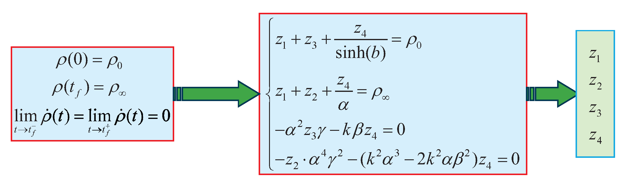
In order to establish an intuitive and clear relationship between controller design and performance such as overshoot, convergence time, accuracy, etc, prescribed performance control (PPC) has gradually gained attention [13]. Moreover, PPC is not completely independent of the above existing control methods. It provides a framework that can be integrated into them for performance-constrained design. For the purpose of providing a desirable transient and steady performance, PPC has been implemented by using the prescribed performance function, whose shapes can be designed as needed to regulate the error. Ref. [14] implemented PPC for combined spacecraft control, but the performance constraints were poor. Although [15,16,17] improves finite time convergence, it lacks the ability to adapt to disturbances. Ref. [18] avoids control singularity through mapping transformation, but its design is difficult and it is still a static function. Ref. [19] designed a performance function adaptive correction method to accommodate small disturbances, but still cannot handle large-scale faults, which refer to actuator faults exceeding saturation level. In [20], PPC has been improved to handle non-continuous control references. The tunnel prescribed performance function was designed in [21], which can better constrain overshoot but does not have dynamic adjustment capabilities. However, PPC still has problems such as over-reliance on initial error prior information and an inability to adaptively adjust static performance envelopes [18,22]. Actuator faults exceeding saturation levels degrade tracking performance and cause input saturation, leading to increased tracking errors and control singularities. As errors breach the fixed performance envelope, control inputs accumulate, further saturating the actuators. Additionally, enhancing PPC to avoid repetitive envelope initialization and improve its generality is a key challenge. This paper addresses these issues by proposing the adhesive-resilient prescribed control (ARPC), which improves robustness and adaptability, particularly in the presence of actuator faults and varying initial conditions.

On the other hand, as spacecraft subsystems grow in number and integration, communication demands between modules rise, yet resources and energy remain constrained. Excessive data transmission risks congestion and safety hazards. Thus, minimizing the communication usage of the ACS to alleviate module congestion is of significant research value. All aforementioned control methods are developed based on the continuous time framework. In current digital computers, signals need to be transmitted continuously with a sufficiently small sampling period. In order to alleviate the increasingly serious communication congestion problem, the event trigger (ET) scheme has been widely studied [23,24]. An ET scheme with a relative threshold based on the control error was designed in [25]. Another relative threshold ET scheme based on sliding mode error is given in [26,27]. ET control based on fixed thresholds [28,29] was developed, but it lacks the ability to adapt to different degrees of control error. Ref. [30] designed a 1-bit based ET scheme, which tries to explore a balance between reducing transmission and performance, but the single updating strategy leads to less-than-ideal accuracy, and there is still room for improvement and expansion. Fixed thresholds lack adaptive capabilities, and relative thresholds are prone to signal distortion [31]. ET and PPC are combined [32,33] to achieve event-triggered control of performance constraints. It is important to note that these combinations involve a trade-off, sacrificing certain performance aspects in order to reduce communication frequency, a limitation imposed by the adopted ET scheme. Moreover, prior research has predominantly concentrated on minimizing communication frequency, without addressing the design of more intricate multi-step thresholds or the optimization of the number of bits needed for each transmission.

To mitigate the performance degradation of ACS caused by actuator faults, active fault-tolerant control is an effective method to ensure stable operation under non-fatal faults [34]. However, when implemented within active fault-tolerant control laws, PPC encounters challenges such as control singularity and limited adaptability to arbitrary initial conditions. Furthermore, existing event-triggered (ET) schemes often struggle to balance performance constraints with minimal communication usage. Motivated by these issues, this paper explores the development of dynamic adaptive PPC to address faults or disturbances exceeding saturation levels, and designs an adhesive initial performance envelope to avoid complex parameter adjustments. Additionally, we extend the recent results from the author’s team [31] to address the integration of prescribed performance control singularity under actuator faults in spacecraft attitude control, effectively reducing communication congestion and minimizing transmission bits. The contributions of this paper can be summarized as follows:

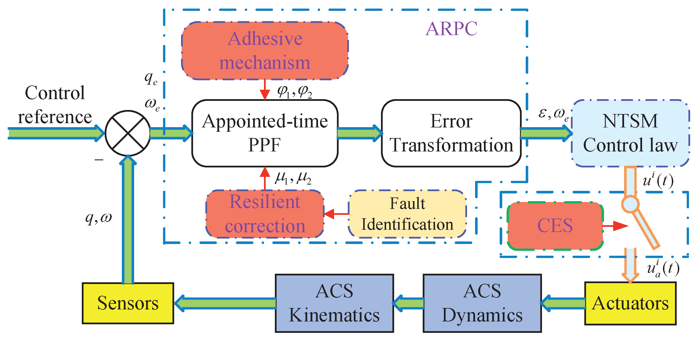
• Adhesive-resilient prescribed control (ARPC) is proposed to effectively resolve prescribed control singularities. By sensing faults, saturation, and error trends, it adaptively applies resilient corrections. To prevent boundary breaches, resilient envelopes are proactively relaxed, with higher-performance envelopes reinstated when conditions allow. This method transforms traditional static PPC into a dynamic approach. Compared to [14,19], ARPC significantly reduces control singularity and conservatism, greatly enhancing robustness.
• The proposed ARPC incorporates an adhesive mechanism that automatically adjusts the initial performance envelope to accommodate arbitrary initial errors. This flexibility allows ARPC to handle any initial conditions without compromising transient performance and reduces reliance on initial errors. Compared with [18,24], it prevents control singularities and simplifies initial parameter design, thereby greatly enhancing its general applicability.
• The CES dynamically updates control outputs by transmitting compressed z-ary bits through a flexible triggering strategy. Compared to other ET schemes [25,28], it minimizes communication frequency between the control box and actuator, significantly reducing data transmission. This alleviates communication congestion, extends actuator lifespan, and balances resource conservation with high control performance.

This paper is organized as follows: Section 2 presents the system models, preliminaries, and control objectives for spacecraft ACS. Section 3 is dedicated to the main contributions of this work. Section 4 demonstrates the effectiveness and superiority of the proposed scheme through numerical simulation comparison. Finally, the conclusion of this study is given in Section 5.

2. Problem Statement and Preliminaries

Considering the singularity problem when using Euler angles to describe the large-scale agile maneuvering of the spacecraft, quaternions will be used here to describe it. The spacecraft attitude kinematic equation is expressed as follows [35,36]:

$${\dot{q}}_0=-{\displaystyle \frac{1}{2}}{{\mathit{q}}_{\mathit{v}}}^{\mathrm{T}}\mathit{\omega },{\dot{\mathit{q}}}_v={\displaystyle \frac{1}{2}}({{\mathit{q}}_{\mathit{v}}}^{\times }+q_0{I}_3)\mathit{\omega }$$

(1)

in which $q_0,{\mathit{q}}_{\mathit{v}}$ are the scalar and vector parts of the quaternion $\mathit{q}$; $\mathit{q}={[q_0,{{\mathit{q}}_{\mathit{v}}}^{\mathrm{T}}]}^{\mathrm{T}}$ is a unit quaternion used to describe the attitude of the spacecraft body coordinate system $\mathbb{B}$ relative to the inertial coordinate system $\mathbb{I}$, and satisfies ${∥\mathit{q}∥}_2=1$; $\mathit{\omega }\in R^{3\times 1}$ represents the attitude angular rate of the spacecraft in $\mathbb{B}$ relative to $\mathbb{I}$; and $I_3\in R^{3\times 3}$ is the identity matrix. ${(·)}^{\times }$ is a tilde matrix operation expressed as follows:

$$a={\left[a_1,a_2,a_3\right]}^{\mathrm{T}},a^{\times }=\left[\begin{array}{ccc}0& -a_3& a_2\\ a_3& 0& -a_1\\ -a_2& a_1& 0\end{array}\right]$$

(2)

The spacecraft attitude dynamics [37] equation can be expressed as:

$$J\dot{\mathit{\omega }}=-{\mathit{\omega }}^{\times }J\mathit{\omega }+(D_0+\Delta D)\mathit{u}+{\mathit{u}}_f+\mathit{d}$$

(3)

where $J=J_0+\Delta J\in R^{3\times 3}$ represents the spacecraft’s actual moment of inertia matrix, $J_0$ and $\Delta J$ are the nominal part and uncertainty, respectively [38]. Similarly, $D_0$ is the nominal actuator configuration matrix, and $\Delta D$ is its uncertainty part. ${\mathit{u}}_f\in R^{3\times 1}$ indicates actuator additive fault; $\mathit{d}$ is the disturbance torque on the spacecraft, mainly from gravity gradient, solar pressure, atmospheric drag and space magnetic field. $\mathit{u}={[\mathrm{sat}\left(u_1\right),\mathrm{sat}\left(u_2\right),\cdots ,\mathrm{sat}\left(u_n\right)]}^{\mathrm{T}}\in R^{n\times 1}$ is the output torque of n actuators, and $\mathrm{sat}(·)$ can be expressed as follows:

$$\mathrm{sat}\left(u_i\right)=\left\{\begin{array}{cc}{u}_i\hfill & ,\left|u_i\right|<u_{max}\hfill \\ sign\left(u_i\right)·u_{max}\hfill & ,\left|u_i\right|\ge u_{max}\hfill \end{array}\right.i=1,2,\cdots ,n$$

(4)

After appropriate transformation, (3) can be expressed more specifically as follows:

$$\begin{array}{cc}\hfill & J_0\dot{\mathit{\omega }}=-{\mathit{\omega }}^{\times }{J}_0\mathit{\omega }+D_0\mathit{u}+\mathit{f}\hfill \end{array}$$

(5)

$$\mathit{f}=J_0\overline{J}[-{\mathit{\omega }}^{\times }J\mathit{\omega }+(D+\Delta D)\mathit{u}+{\mathit{u}}_f+\mathit{d}]-{\mathit{\omega }}^{\times }\Delta J\mathit{\omega }+\mathit{d}+\Delta D\mathit{u}$$

(6)

where $\mathit{f}$ represents equivalent faults including faults, uncertainties and disturbances, making it easier to design and implement fault-tolerant control laws; in addition, $\overline{J}=-{(J_0+J_0\Delta J^{-1}{J}_0)}^{-1}$.

To achieve attitude tracking control, it is necessary to further transform (6) into the error dynamics equation. Define ${\mathit{q}}_d$ as the desired attitude quaternion, then the error quaternion of $\mathbb{B}$ relative to target coordinate system $\mathbb{D}$ can be expressed as ${\mathit{q}}_e={[q_{e0},{\mathit{q}}_{ev}^{\mathrm{T}}]}^{\mathrm{T}}={\mathit{q}}_d^{-1}\odot \mathit{q}$, where ⊙ is the quaternion multiplication operation. ${\mathit{\omega }}_e=\mathit{\omega }-C{\mathit{\omega }}_d$ represents the angular velocity error of $\mathbb{B}$ relative to $\mathbb{I}$, where ${\mathit{\omega }}_d$ is the desired angular velocity, $C=(q_{e0}^2-{\mathit{q}}_{ev}^{\mathrm{T}}{\mathit{q}}_{ev})I_3+2{\mathit{q}}_{ev}{\mathit{q}}_{ev}^{\mathrm{T}}-2q_{e0}{\mathit{q}}_{ev}^{\times }$ denotes the corresponding rotation matrix between $\mathbb{B}$ and $\mathbb{D}$. Then the ACS error dynamics is further given by

$$\begin{array}{cc}\hfill & {\dot{q}}_{e0}=-{\displaystyle \frac{1}{2}}{\mathit{q}}_{ev}^{\mathrm{T}}{\mathit{\omega }}_e,{\dot{\mathit{q}}}_{ev}={\displaystyle \frac{1}{2}}({\mathit{q}}_{ev}^{\times }+q_{e0}{I}_3){\mathit{\omega }}_e\hfill \\ \hfill J_0{\dot{\mathit{\omega }}}_e=& -{\mathit{\omega }}^{\times }{J}_0\mathit{\omega }+J_0({\mathit{\omega }}_e^{\times }C{\mathit{\omega }}_d-C{\dot{\mathit{\omega }}}_d)+D_0\mathit{u}+\mathit{f}\hfill \end{array}$$

(7)

Assumption 1.

The set $\mathit{f}$ of faults, uncertainties, and disturbances is bounded, i.e., $∥\mathit{f}∥\le \overline{f}$ [12]. This is because the nominal model accuracy is relatively high and the magnitude of spatial environmental disturbances is small. Actuator faults cannot be unbounded due to physical energy limitations.

Assumption 2.

The fault estimate $\widehat{\mathit{f}}$ can be obtained through an observer or filter, and the estimation error is bounded, satisfying $\tilde{\mathit{f}}=\mathit{f}-\widehat{\mathit{f}}\le ∥\tilde{\mathit{f}}∥$. There is abundant research on fault estimation (reconstruction). Limited by space, this paper does not involve how to design fault estimation algorithms. For more details, please refer to previous research from the author’s team [39] or other results [40], etc.

Assumption 3.

The spacecraft attitude angle $\mathit{q}$ and attitude angular rate ω can be measured, the feedback control law can be designed based on $\mathit{q}$ and ω, and the desired angular velocities ${\mathit{\omega }}_d$ and ${\dot{\mathit{\omega }}}_d$ are bounded [15].

To achieve fault tolerance, it is necessary to ensure that the attitude remains stable and controllable under fault conditions. To facilitate the description of the control objectives and problems, the issue can be roughly divided into two cases. One is that the fault is smaller than the output capacity of the actuator, that is, $\left|f\right|\le u_{max}$. Once the fault is accurately identified, it can be easily offset by the fault-tolerant control law. The other is that when the fault exceeds the output capacity of the actuator $\left|f\right|>u_{max}$, the actuator is not sufficient to generate the torque to offset the fault, which inevitably causes the posture to deviate from the ideal trajectory. When Assumptions 1 and 3 do not hold, the proposed method will lose stability. When Assumption 2 does not hold, the compensation effect of active fault tolerance will be greatly reduced.

3. Adhesive-Resilient Prescribed Control with CES

This section mainly introduces the proposed adhesive-resilient prescribed control (ARPC) for spacecraft with a compression event-triggered scheme (CES), which mainly consists of three parts. The first is the design of ARPC under large-scale faults and arbitrary initial conditions. The second is the design of fault-tolerant control law based on ARPC. The third is the design of a compression event-triggered scheme (CES). The overall structural relationship of ARPC and CES is shown in Figure 1.

3.1. Design of ARPC

In existing results, the prescribed performance function usually converges from ${\rho }_0$ to ${\rho }_{\infty }$ in an exponential law as $\rho \left(t\right)={\rho }_0{e}^{-kt}+{\rho }_{\infty }$, which is a static function that cannot be modified in real time during the control process. It has the problems of difficult parameter design, strong conservatism, and an inability to handle large disturbances, resulting in control singularity. To solve the above problems, this section presents a novel design method of ARPC.

First of all, to achieve the appointed time convergence, this section proposes a novel appointed-time performance function, with its design method outlined as follows:

$$\rho \left(t\right)=z_1+z_2·sin({\displaystyle \frac{\pi t}{2t_f}})+z_3·cos({\displaystyle \frac{\pi t}{2t_f}})+{\displaystyle \frac{z_4}{sinh(kt+b)}}$$

(8)

where $t_f$ represents the appointed time, which is the convergence time specified by the user to determine when $\rho \left(t\right)$ converges to ${\rho }_{\infty }$; and $z_1,z_2,z_3,z_4$ are the parameters to be designed. Let $\alpha =sinh(k{t}_f+b),\beta =cosh(k{t}_f+b),\gamma =\pi /2t_f$, then $z_i,i=1,2,3,4$ can be obtained as follows:

$$\begin{array}{cc}\hfill z_4& ={\displaystyle \frac{({\rho }_0-{\rho }_{\infty }){\gamma }^2{\alpha }^{4}sinh\left(b\right)}{(k^2{\alpha }^3-2k^2\alpha {\beta }^2-k\beta \gamma {\alpha }^2-{\gamma }^2{\alpha }^3)sinh\left(b\right)+1}},z_3=-{\displaystyle \frac{k\beta z_4}{\gamma {\alpha }^2}}\hfill \\ \hfill z_2& ={\displaystyle \frac{(2k^2\alpha {\beta }^2-k^2{\alpha }^3)z_4}{{\gamma }^2{\alpha }^4}},z_1={\rho }_0-{\displaystyle \frac{z_4}{sinh\left(b\right)}}-z_3\hfill \end{array}$$

(9)

According to the basic properties, The conditions that performance function must meet are listed on the left side of the Figure 2. The equation relationship in the middle of the figure can be further obtained, and by solving it, $z_i,i=1,2,3,4$ can be determined.

Based on the given appointed-time performance function in (8), the resilient envelopes can be further designed as:

$$\begin{array}{cc}\hfill & {\rho }_d\left(t\right)<e\left(t\right)<{\rho }_u\left(t\right)\hfill \\ \hfill {\rho }_d\left(t\right)& =[a-sign\left(e_0\right)]\rho \left(t\right)+{\rho }_{\infty }·sign\left(e_0\right)+{\mu }_1\left(t\right)-{\phi }_1\left(t\right)\hfill \\ \hfill {\rho }_u\left(t\right)& =[a+sign\left(e_0\right)]\rho \left(t\right)-{\rho }_{\infty }·sign\left(e_0\right)+{\mu }_2\left(t\right)+{\phi }_2\left(t\right)\hfill \end{array}$$

(10)

in which ${\rho }_d\left(t\right),{\rho }_u\left(t\right)$ are the lower bound and upper bound of the resilient envelopes, respectively; a is a parameter given by the user that can change the shape of the boundary; ${\mu }_1\left(t\right)$ and ${\mu }_2\left(t\right)$ are adaptive resilient correction terms; and ${\phi }_1\left(t\right),{\phi }_2\left(t\right)$ is an adhesive mechanism can automatically attached to any initial error, avoiding the problem that the performance constraint interval cannot be accurately captured in complex working conditions. Therefore, (8) can be transformed from a static to a dynamic function for handling faults exceeding the saturation level through correction.

The design method of the resilient correction term ${\mu }_1\left(t\right),{\mu }_2\left(t\right)$ is further given as follows:

$$\begin{array}{cc}\hfill {\mu }_1\left(t\right)& =-{\kappa }_1·tanh\left(\mu \left(t\right)\right),{\mu }_2\left(t\right)={\kappa }_2·tanh\left(\mu \left(t\right)\right)\hfill \\ \hfill \mu \left(t\right)=& {\int }_0^t[{\delta }_1·\nu \left(\sigma \right)+{\delta }_2·{\dot{q}}_{ev}\left(\sigma \right)-{\delta }_3{\displaystyle \frac{\mu \left(\sigma \right)}{\left|\mu \left(\sigma \right)\right|+{\delta }_4}}]d\sigma \hfill \\ \hfill \nu \left(\sigma \right)& =\left\{\begin{array}{cc}sign\left(\widehat{f}\left(\sigma \right)\right)·[u_{max}-\widehat{f}\left(\sigma \right)]\hfill & ,\left|\widehat{f}\left(\sigma \right)\right|>u_{max}\hfill \\ 0\hfill & ,\left|\widehat{f}\left(\sigma \right)\right|\le u_{max}\hfill \end{array}\right.\hfill \end{array}$$

(11)

where $\mu \left(t\right)$ is the intermediate variable and $\mu \left(0\right)=0$; ${\delta }_i,i=1,2,3,4$ are positive definite gain parameter that defines the decay rate; and ${\kappa }_1,{\kappa }_2$ are positive definite gain parameters that determines the resilient amplitude. $\nu \left(\sigma \right)$ is the virtual saturation; $\widehat{f}\left(\sigma \right)$ is the estimation of the lumped fault $f\left(\sigma \right)$ from the fault diagnosis module; and ${\mu }_1\left(t\right),{\mu }_2\left(t\right)$ are respectively generated according to the virtual saturation, attitude error change rate, and corresponding gain parameters generated by the virtual control law to generate time-varying resilient correction terms for the dynamic correction of $\rho \left(t\right)$.

The design of ${\phi }_1\left(t\right),{\phi }_2\left(t\right)$ is further given as:

$$\begin{array}{cc}\hfill & {\phi }_1\left(t\right)=\left\{\begin{array}{cc}[e_0-{\displaystyle \frac{\lambda {\rho }_2\left(0\right)+(\lambda -2){\rho }_1\left(0\right)}{2}}]·{(1-\nu \vartheta t)}^{{\displaystyle \frac{1}{\nu }}}\hfill & ,0\le t\le t_f\hfill \\ 0\hfill & ,t>t_f\hfill \end{array}\right.\hfill \\ \hfill & {\phi }_2\left(t\right)=\left\{\begin{array}{cc}[e_0+{\displaystyle \frac{(\lambda -2){\rho }_2\left(0\right)+\lambda {\rho }_1\left(0\right)}{2}}]·{(1-\nu \vartheta t)}^{{\displaystyle \frac{1}{\nu }}}\hfill & ,0\le t\le t_f\hfill \\ 0\hfill & ,t>t_f\hfill \end{array}\right.\hfill \end{array}$$

(12)

where $\nu$ is a positive constant; $t_f$ is the terminal time specified by the user; and $\vartheta ={\displaystyle \frac{1}{t_f\nu }}$.

Remark 1.

Theoretically, $t_f$ in (12) can be chosen arbitrarily, but usually, to ensure that the transient performance is not affected by the modification of the adhesive mechanism ${\phi }_1\left(t\right),{\phi }_2\left(t\right)$, the choice of in (12) is kept consistent with ${\rho }_1\left(t\right),{\rho }_2\left(t\right)$ in (10).

In order to intuitively demonstrate the role of resilient correction, Figure 3 includes the effects of traditional static performance function and performance function in (10) under the same large-scale fault.

Among them, (a) does not have dynamic adaptive capability. When the actuator is not enough to offset the error increase caused by the fault, it inevitably causes the error to break through the static envelope, thus causing control singularity in the PPC. In contrast, the envelope ${\rho }_u\left(t\right),{\rho }_d\left(t\right)$ of the (10) in (b) can be adaptively widened and tightened again when the fault weakens to an appropriate level, effectively avoiding the above problems.

In order to show how the adhesive mechanism ${\phi }_1\left(t\right),{\phi }_2\left(t\right)$ works, the comparisons before and after the improvement when facing different initial errors are shown in Figure 3. The parameters are selected as $t_f=8$, $k=0.01,b=0.9$, $a=0.2$, $\lambda =3$ and $\nu =0.4$. It can be clearly seen from the left side that (c) lacks an adhesive mechanism, which causes $e\left(t\right)$ to break the constraints of the performance envelope and lead to a singularity. In contrast, the right side (d) increases the effect of adhesive mechanism and uses the correction of ${\phi }_1\left(t\right),{\phi }_2\left(t\right)$ to obtain new performance envelopes. The original boundary is appropriately modified so that $e\left(0\right)$ can accurately fall into the constraint interval, and constraints are imposed on $e\left(t\right)$ until it enters the original allowed interval. When $t\ge t_f$, the adhesive mechanism no longer works, causing $e\left(t\right)$ to enter a steady state. Through the above improvements, it is ensured that ${\rho }_d\left(t\right)<e\left(t\right)<{\rho }_u\left(t\right)$ is satisfied at all times, avoiding singularity, which can greatly reduce manual intervention in parameter design.

3.2. Design of Fault-Tolerant Control Law Based on ARPC

After solving how to design a more robust and less conservative PPC, this section will further develop fault-tolerant control law on the basis of ARPC.

Define the error quaternion ${\mathit{q}}_{ev}\left(t\right)$ as the tracking error $\mathit{e}\left(t\right)$; that is, it is necessary to design an appropriate fault-tolerant control law so that the following constraint is satisfied.

$${\rho }_d\left(t\right)<q_{ei}\left(t\right)<{\rho }_u\left(t\right),i=1,2,3$$

(13)

First, the performance function used as a constraint tool for tracking error has been defined in (8)–(20). However, (13) presents an inequality constraint on the error variable, making it challenging to directly design the controller. To reduce this complexity, the following error transformation function is introduced, which converts the constrained error variable into an unconstrained one.

$$\mathit{\epsilon }\left(t\right)=ln{\displaystyle \frac{{\mathit{q}}_{ev}\left(t\right)-{\mathit{\rho }}_d\left(t\right)}{{\mathit{\rho }}_u\left(t\right)-{\mathit{q}}_{ev}\left(t\right)}}$$

(14)

where $\mathit{\epsilon }\left(t\right)$ represents the unconstrained error, and the transformed error $\mathit{\epsilon }\left(t\right)$ obtained after the above error transformation is not constrained; that is, $\mathit{\epsilon }\left(t\right)\in (-\infty ,+\infty )$. By converting the error variable constrained by the inequality into an unconstrained error variable in the above way, the complexity of the controller design is greatly reduced. Moreover, since the error transformation belongs to a differential homeomorphism transformation, when a reasonable control law is designed to make the variable error $\mathit{\epsilon }\left(t\right)$ bounded, the real error ${\mathit{q}}_{ev}\left(t\right)$ is also bounded, and it will also meet the prescribed performance constraints.

At the same time, the first-order derivative of $\mathit{\epsilon }\left(t\right)$ is obtained, which will be used for the subsequent control law design. For simplicity and ease of writing, $\left(t\right)$ is omitted here.

$$\dot{\mathit{\epsilon }}={\displaystyle \frac{({\mathit{\rho }}_u-{\mathit{\rho }}_d){\dot{\mathit{q}}}_{ev}+{\mathit{\rho }}_d{\dot{\mathit{\rho }}}_u-{\dot{\mathit{\rho }}}_d{\mathit{\rho }}_u+({\dot{\mathit{\rho }}}_d-{\dot{\mathit{\rho }}}_u){\mathit{q}}_{ev}}{({\mathit{\rho }}_u-{\mathit{q}}_{ev})({\mathit{q}}_{ev}-{\mathit{\rho }}_d)}}$$

(15)

Next, consider constructing the following non-singular terminal sliding surface:

$$\mathit{s}\left(t\right)=k_{1}si{g}^{{\displaystyle \frac{p}{q}}}\left(\mathit{\epsilon }\left(t\right)\right)+{\mathit{\omega }}_e\left(t\right)$$

(16)

in which $k_1$ is a positive scalar; and p and q are both positive odd numbers and satisfy $1<{\displaystyle \frac{p}{q}}<2$. In addition, $si{g}^{{\displaystyle \frac{p}{q}}}(·)={\left|·\right|}^{{\displaystyle \frac{p}{q}}}sign(·)$. For the convenience of writing, is omitted here. Taking the derivative of (16), the following result can be obtained:

$$J_0\dot{\mathit{s}}=J_0{k}_1{\displaystyle \frac{p}{q}}diag({\left|\mathit{\epsilon }\right|}^{{\displaystyle \frac{p}{q}}-1})\dot{\mathit{\epsilon }}+J_0{\dot{\mathit{\omega }}}_e$$

(17)

Substituting (7) into the above equation, it is easy to obtain:

$$J_0\dot{\mathit{s}}=-{\mathit{\omega }}^{\times }{J}_0\mathit{\omega }+J_0({\mathit{\omega }}_e^{\times }C{\mathit{\omega }}_d-C{\dot{\mathit{\omega }}}_d)+D_0\mathit{u}+\mathit{f}+J_0{k}_1{\displaystyle \frac{p}{q}}diag({\left|\mathit{\epsilon }\right|}^{{\displaystyle \frac{p}{q}}-1})·\dot{\mathit{\epsilon }}$$

(18)

In order to make ACS approach the equilibrium point within a finite time and maintain the sliding mode motion in the sliding-mode arrival stage, the following fast terminal sliding-mode approach law is selected:

$$\dot{\mathit{s}}=J_0^{-1}(-k_{2}s-k_3{sig}^{\chi }\left(\mathit{s}\right))$$

(19)

similarly, $\chi \in (0,1)$; and $k_2,k_3$ are positive scalars.

Combining the above formula and (18), the fault-tolerant control law can be designed as follows:

$$\begin{array}{cc}\hfill & \mathit{u}=D_0^{†}[-{\mathit{\omega }}^{\times }{J}_0\mathit{\omega }+J_0({\mathit{\omega }}_e^{\times }C{\mathit{\omega }}_d-C{\dot{\mathit{\omega }}}_d)-\widehat{\mathit{f}}+J_0{k}_1{\displaystyle \frac{p}{q}}diag({\left|\mathit{\epsilon }\right|}^{{\displaystyle \frac{p}{q}}-1})\dot{\mathit{\epsilon }}]+{\mathit{u}}_s\hfill \\ \hfill & \mathrm{with}{\mathit{u}}_s=\left\{\begin{array}{cc}{D}_0^{†}(-k_2\mathit{s}-k_3{sig}^{\chi }\left(\mathit{s}\right))\hfill & ,∥\mathit{s}∥\ge \zeta \hfill \\ 0\hfill & ,∥\mathit{s}∥<\zeta \hfill \end{array}\right.\hfill \end{array}$$

(20)

where $D_0^{†}=D_0^{\mathrm{T}}{\left(D_0{D}_0^{\mathrm{T}}\right)}^{-1}$ is the pseudo-inverse matrix of $D_0$; and $\widehat{\mathit{f}}$ represents the estimation of the equivalent fault $\mathit{f}$.

3.3. Design of z-Ary Compression Event-Triggered Scheme

To achieve an optimal balance between communication transmission consumption and performance, a z-ary compression event-triggered scheme is introduced to modify the controller. The CES update strategy is designed as follows:

$$\begin{array}{cc}\hfill & v\left(t\right)=u\left(t_k\right),\forall t\in [t_k,t_{k+1}),k=0,1,\cdots \hfill \\ \hfill & t_{k+1}=inf\{t>t_k|\left|v\left(t\right)-u\left(t\right)\right|\ge o{z}^h\}\hfill \end{array}$$

(21)

where $u\left(t\right)$ is the designed control law; $\Delta v\left(t\right)=u\left(t\right)-v\left(t\right)$ represents the control signal error; $t_k$ is the update time; and z is an arbitrary even number specified by the user. Figure 4 shows the update strategy of CES and its general operating mechanism.

Different from the traditional fixed threshold event trigger mechanism, the control input is divided into different intervals here, and different step thresholds are designed based on this. First, $0=u_{v|0}<u_{v|1}<\cdots <u_{v|l}=u_{max}$ is used as the interval to divide the control input $u\left(t\right)$ into l different intervals to measure the relative size of $u\left(t\right)$, where $l={\displaystyle \frac{z^m}{2}}-1$. m is the length of the transfer bits specified by the user; that is, a single transmission requires m bytes. According to the judgment of which interval $u\left(t\right)$ belongs to at different times, $o,h$ can be determined according to the following rules.

$$if\left|u\left(t\right)\right|\in [u_{v|j},u_{v|j+1})\Rightarrow h=j\Rightarrow \left\{\begin{array}{cc}{\sum }_{r=1}^m{s}_{r,k}{z}^{r-1}=h\hfill & ,s_{1,k}<{\displaystyle \frac{z}{2}}\hfill \\ {\sum }_{r=1}^m{s}_{r,k}{z}^{r-1}-{\displaystyle \frac{z^m}{2}}=h\hfill & ,s_{1,k}\ge {\displaystyle \frac{z}{2}}\hfill \end{array}\right.$$

(22)

where $s_{r,k}\in \{0,1,\cdots ,z-1\}$ represents each byte of the z-ary number system at the k-th update time. All $s_{r,k}$ are combined in sequence to obtain the bits that need to transmit when updating the control signal, which can be specifically written as $S_k=s_{1,k}{s}_{2,k}\cdots s_{m-1,k}{s}_{m,k}$; and $o_j,j=0,1,\cdots ,l$ is the coefficient to be designed, which is used to realize compression and decompression.

From the trigger conditions, it can be seen that the same value of $\left|v\left(t\right)-u\left(t\right)\right|$ may represent two control directions. Let $v\left(t\right)-u\left(t\right)\ge 0,s_{1,k}<{\displaystyle \frac{z}{2}}$, otherwise there is $v\left(t\right)-u\left(t\right)<0,s_{1,k}\ge {\displaystyle \frac{z}{2}}$. This relationship is used to ensure that symbols can be accurately judged during compression and decompression; that is, the direction can be controlled.

Once the trigger condition in (21) is met, the data bus transmits the bit $S_k$ to the actuators. With the help of the trigger mechanism and the compression, $S_k$ can be regarded as the sign and magnitude representation of the trigger error $u\left(t\right)-v\left(t\right)$ threshold. More specifically, the first byte $s_{m,k}$ represents the sign bit, while the magnitude is determined by the remaining bytes $s_{m-1,k},\cdots ,s_{1,k}$. As shown in

Table 1. Compression and decompression examples when $z=2,m=3$.

Compressed Bits	Decompression Parameters
$S_k=000$	Positive $s_{1,k}<{\displaystyle \frac{z}{2}}$	$h=0$	$o=o_0$
$S_k=001$		$h=1$	$o=o_1$
$S_k=010$		$h=2$	$o=o_2$
$S_k=011$		$h=3$	$o=o_3$
$S_k=100$	Negative $s_{1,k}\ge {\displaystyle \frac{z}{2}}$	$h=0$	$o=o_1$
$S_k=101$		$h=1$	$o=o_2$
$S_k=110$		$h=2$	$o=o_3$
$S_k=111$		$h=3$	$o=o_4$

, specific compression and decompression is demonstrated by taking $z=2,m=3$ as an example.

When the actuator receives $S_k$, it uses the following decompression to update $u_d\left(t\right)$ with the help of the last updated control signal and the stored compression and decompression parameters:

$$v_a\left(t\right)=v\left(t_k\right)=\left\{\begin{array}{cc}v\left(t_{k-1}\right)+o{z}^h\hfill & ,s_{m,k}<z/2\hfill \\ v\left(t_{k-1}\right)-o{z}^h\hfill & ,s_{m,k}\ge z/2\hfill \end{array}\right.$$

(23)

in which the selection of $o,z,h$ follows the same rules in (21) and (22), which are also stored in the actuators. Based on the triggering condition in (22) and the decompression rule in (23), it can be deduced that $v\left(t\right)=v_a\left(t\right)$. Larger z and m means more complex and fine interval division, and also means longer bytes. This will lead to more precise control updates, but also means more frequent triggers and more transmission data.

In order to verify that the Zeno phenomenon does not occur, the time derivative of $v\left(t\right)$ before the next trigger is given:

$$\Delta \dot{u}\left(t\right)=\dot{u}\left(t\right)-\dot{u}\left(t_k\right)=\dot{u}\left(t\right),t_k\le t<t_{k+1}$$

(24)

where $k=1,2,\cdots$. By invoking the control law, given Assumptions 1–3, and the fact that $q_{ev}\left(t\right)$ and its derivatives under $u\left(t\right)$ satisfy the bounded conditions under the constraint of ${\rho }_d\left(t\right),{\rho }_u\left(t\right)$, it can be seen that the boundedness of $\left|\dot{u}\left(t\right)\right|$ is guaranteed. For ease of expression, the upper bound is defined as $\overline{u}$, so the following can be obtained:

$$\left|\dot{u}\left(t\right)\right|\le \overline{u},t_k\le t<t_{k+1}$$

where $k=1,2,\cdots$, given ${lim}_{t\to t_k^{+}}\left|u\left(t\right)-u\left(t_k\right)\right|=0$ and ${lim}_{t\to t_{k+1}^{-}}\left|u\left(t\right)-u\left(t_k\right)\right|=o{z}^h$, shows that there exists a strictly positive constant such that $t_{k+1}-t_k\ge {\displaystyle \frac{o{z}^h}{\left|\overline{u}\right|}}$.

3.4. Stability Analysis

Then, Lyapunov stability analysis is performed on the proposed control law with the CES scheme.

Theorem 1.

For the mathematical model of spacecraft attitude tracking with actuator faults and disturbance (7), under the conditions of satisfying Assumptions 1–3, the designed control law in (20) with CES in (21) ensures that the equivalent error converges in a finite time. The transformed attitude tracking errors (14) can be used to guarantee the tracking errors ${\mathit{q}}_{ev}$ converge within the ARPC envelopes in (13).

Lemma 1.

Consider a nonlinear system, assuming that there exists a continuous differentiable function $V\left(x\right)$ defined in a neighborhood containing the origin that satisfies $\dot{V}\left(x\right)\le -{\lambda }_{1}V\left(x\right)-{\lambda }_2{V}^k\left(x\right)$. Then the state can reach the origin in a finite time, and the convergence time T satisfies $T\le {\lambda }_1^{-1}{(1-k)}^{-1}ln(1+{\lambda }_1{\lambda }_2^{-1}{V}_0^{1-k})$. Among them, ${\lambda }_1,{\lambda }_2,k$ are positive scalars, and $0<k<1$.

Proof. 

Then, take $V_1={\displaystyle \frac{1}{2}}{\mathit{s}}^{\mathrm{T}}{J}_0\mathit{s}$ as the Lyapunov function, obtain its derivative and invoke (18) to obtain

$${\dot{V}}_1={\mathit{s}}^{\mathrm{T}}{J}_0\dot{\mathit{s}}={\mathit{s}}^{\mathrm{T}}(-{\mathit{\omega }}^{\times }{J}_0\mathit{\omega }+J_0({\mathit{\omega }}_e^{\times }C{\mathit{\omega }}_d-C{\dot{\mathit{\omega }}}_d)+D_0\mathit{u}+\mathit{f}+J_0{k}_1{\displaystyle \frac{p}{q}}diag({\left|\mathit{\epsilon }\right|}^{{\displaystyle \frac{p}{q}}-1})·\dot{\mathit{\epsilon }})$$

(25)

Substitute (20) into the above equation, taking into account the update error $\Delta \mathit{v}$ caused by CES. According to the definition of $\Delta v^i$, it can be obtained that $\Delta v^i\left(t\right)=u^i\left(t\right)-{\mathit{v}}^i\left(t\right)$, $\left|\Delta v^i\right|\le {\overline{z}}^i$, where ${\overline{z}}^i=max\{o_0{\left(z_i\right)}^0,o_1{z}_i,\cdots ,o_{l+1}{\left(z_i\right)}^{l+1}\}$ is a positive constant.

$$\begin{array}{cc}\hfill {\dot{V}}_1& ={\mathit{s}}^{\mathrm{T}}(\tilde{\mathit{f}}+∥\Delta \mathit{v}∥-k_2\mathit{s}-k_3{sig}^{\chi }\left(\mathit{s}\right))\hfill \\ \hfill & \le -k_2{∥\mathit{s}∥}^2-k_3{∥\mathit{s}∥}^{\chi +1}+(∥\tilde{\mathit{f}}∥+∥\Delta \mathit{v}∥)∥\mathit{s}∥\hfill \end{array}$$

(26)

where $\tilde{\mathit{f}}=\mathit{f}-\widehat{\mathit{f}}$ represents the estimation error of the lumped fault. It should be noted that usually the fault estimation algorithm will obtain the final upper limit of $\tilde{\mathit{f}}$ during the convergence analysis. This means that this information can be obtained. Note that the control input signal will be updated whenever the CES is triggered, which indicates that $\left|\Delta v^i\right|\le o^i{z}^{h_i}$ holds. As $o,h$ and z are all bounded numbers, it can be derived that ${\overline{z}}^i$ is a bounded constant. So obviously $\Delta \mathit{v}$ is bounded, and $∥\Delta \mathit{v}∥\le \overline{z}$ holds.

Further, through appropriate scaling, it can be rewritten as an inequality relationship:

$$\begin{array}{cc}\hfill {\dot{V}}_1& \le {\displaystyle \frac{-2}{{\lambda }_{max}\left(J_0\right)}}(k_2-{\displaystyle \frac{∥\tilde{\mathit{f}}∥+∥\Delta \mathit{v}∥}{∥s∥}})V_1-{({\displaystyle \frac{2}{{\lambda }_{max}\left(J_0\right)}})}^{{\displaystyle \frac{\chi +1}{2}}}{k}_3{V}_1^{{\displaystyle \frac{\chi +1}{2}}}\hfill \\ \hfill & \le {\displaystyle \frac{-2k_2}{{\lambda }_{max}\left(J_0\right)}}{V}_1-{({\displaystyle \frac{2}{{\lambda }_{max}\left(J_0\right)}})}^{{\displaystyle \frac{\chi +1}{2}}}(k_3-{\displaystyle \frac{∥\tilde{\mathit{f}}∥+∥\Delta \mathit{v}∥}{{∥\mathit{s}∥}^{\chi }}})V_1^{{\displaystyle \frac{\chi +1}{2}}}\hfill \end{array}$$

(27)

in which ${\lambda }_{max}\left(J_0\right)$ represents the maximum eigenvalue of $J_0$.

Therefore, if appropriate parameters are selected to make $k_2>{\displaystyle \frac{∥\tilde{\mathit{f}}∥+∥\Delta \mathit{v}∥}{∥\mathit{s}∥}}$ and $k_3>{\displaystyle \frac{∥\tilde{\mathit{f}}∥+∥\Delta \mathit{v}∥}{{∥\mathit{s}∥}^{\chi }}}$ hold at the same time, then ${\dot{V}}_1<0$ is satisfied. The sliding mode will converge to the following region U in a finite time.

$$\begin{array}{c}\hfill ∥\mathit{s}∥\le U=min\{U_1,U_2\},\mathrm{with}∥\mathit{s}∥\le {\displaystyle \frac{∥\tilde{\mathit{f}}∥+∥\Delta \mathit{v}∥}{k_2}}=U_1,∥\mathit{s}∥\le {({\displaystyle \frac{∥\tilde{\mathit{f}}∥+∥\Delta \mathit{v}∥}{k_3}})}^{{\displaystyle \frac{1}{\chi }}}=U_2\end{array}$$

In addition, the above content satisfies the fast finite time convergence stability condition of Lemma 1, and the state can approach the sliding surface in a finite time. However, it can be seen that this stability condition depends on the upper bound information of the lumped fault.

Lemma 2.

Consider a nonlinear system, assuming that there exists a continuously differentiable function $V\left(x\right)$, and there exist real numbers $\lambda >0,\eta >0,0<\alpha <1$, satisfying (1) $V\left(x\right)$ is positive definite; (2) $\dot{V}\left(x\right)\le -\lambda V^{\alpha }\left(x\right)+\eta$. Then, the system is practically finite-time stable, that is, it reaches the neighborhood of the equilibrium point within a finite time T, and $T\le {\displaystyle \frac{V^{1-\alpha }\left(x_0\right)}{\lambda {\theta }_0(1-\alpha )}}$. Among them $V\left(x_0\right)$ is the initial value of $V\left(x\right)$, and ${\theta }_0$ can take any value in $(0,1)$.

When the error state reaches the sliding surface, the following holds:

$${\mathit{\omega }}_e\left(t\right)=-k_1{sig}^{{\displaystyle \frac{p}{q}}}\left(\mathit{\epsilon }\left(t\right)\right)$$

(28)

In order to further prove the convergence property of the error, the Lyapunov function is selected as $V_2={\displaystyle \frac{1}{2}}{\mathit{\epsilon }}^2$ and its derivative is obtained as follows.

$$\begin{array}{cc}\hfill {\dot{V}}_2& =\mathit{\epsilon }\dot{\mathit{\epsilon }}=\mathit{\epsilon }{\displaystyle \frac{({\mathit{\rho }}_u-{\mathit{\rho }}_d){\dot{\mathit{q}}}_{ev}+{\mathit{\rho }}_d{\dot{\mathit{\rho }}}_u-{\dot{\mathit{\rho }}}_d{\mathit{\rho }}_u+({\dot{\mathit{\rho }}}_d-{\dot{\mathit{\rho }}}_u){\mathit{q}}_{ev}}{({\mathit{\rho }}_u-{\mathit{q}}_{ev})({\mathit{q}}_{ev}-{\mathit{\rho }}_d)}}\hfill \end{array}$$

(29)

$$\begin{array}{cc}\hfill {\dot{V}}_2& ={\displaystyle \frac{\mathit{\epsilon }({\mathit{\rho }}_u-{\mathit{\rho }}_d)}{({\mathit{\rho }}_u-{\mathit{q}}_{ev})({\mathit{q}}_{ev}-{\mathit{\rho }}_d)}}[{\displaystyle \frac{-k_1}{2}}({\mathit{q}}_{ev}^{\times }+q_0{I}_3){sig}^{{\displaystyle \frac{p}{q}}}\left(\mathit{\epsilon }\right)+{\displaystyle \frac{{\mathit{\rho }}_d{\dot{\mathit{\rho }}}_u-{\dot{\mathit{\rho }}}_d{\mathit{\rho }}_u}{{\mathit{\rho }}_u-{\mathit{\rho }}_d}}+{\displaystyle \frac{{\dot{\mathit{\rho }}}_d-{\dot{\mathit{\rho }}}_u}{{\mathit{\rho }}_u-{\mathit{\rho }}_d}}{\displaystyle \frac{e^{\mathit{\epsilon }}{\mathit{\rho }}_u+{\mathit{\rho }}_d}{1+e^{\mathit{\epsilon }}}}]\hfill \\ \hfill & \le -{\displaystyle \frac{k_1}{2}}\Gamma {∥\mathit{\epsilon }∥}^{{\displaystyle \frac{p}{q}}+1}+\Gamma \mathrm{\Theta }∥\mathit{\epsilon }∥+\Gamma {\displaystyle \frac{{\dot{\mathit{\rho }}}_d-{\dot{\mathit{\rho }}}_u}{{\mathit{\rho }}_u-{\mathit{\rho }}_d}}{\displaystyle \frac{e^{\mathit{\epsilon }}{\mathit{\rho }}_u+{\mathit{\rho }}_d}{1+e^{\mathit{\epsilon }}}}∥\mathit{\epsilon }∥\hfill \end{array}$$

where $\Gamma ={\displaystyle \frac{{\mathit{\rho }}_u-{\mathit{\rho }}_d}{({\mathit{\rho }}_u\mathit{-}{\mathit{q}}_{ev})({\mathit{q}}_{ev}-{\mathit{\rho }}_d)}}$; $\mathrm{\Theta }={\displaystyle \frac{{\mathit{\rho }}_d{\dot{\mathit{\rho }}}_u-{\dot{\mathit{\rho }}}_d{\mathit{\rho }}_u}{{\mathit{\rho }}_u-{\mathit{\rho }}_d}}$. Since ${\phi }_1\left(t\right),{\phi }_2\left(t\right)$ only plays the role of initial adhesive, it is equivalent to adjusting the initial parameters to ensure that the initial error is always within the envelope, and its influence can be omitted in the analysis process.

By analyzing the relationship within the inequality one by one, since the constraint relationship ${\mathit{\rho }}_d<{\mathit{q}}_{ev}<{\mathit{\rho }}_u$ holds, it is obvious that $\Gamma >0$. Since there exists $a,\mathit{\rho },{\rho }_{\infty },{\kappa }_1,{\kappa }_2>0$ and $\dot{\mu }\left(t\right)=1-{tanh}^2\left(\mu \right)>0$. By expanding and simplifying, it can be obtained that

$$\mathrm{\Theta }={\displaystyle \frac{[(a({\kappa }_1+{\kappa }_2)+{\kappa }_1-{\kappa }_2)\mathit{\rho }-({\kappa }_1+{\kappa }_2)+2\dot{\mathit{\rho }}]\dot{\mathit{\mu }}+2a\dot{\mathit{\rho }}{\rho }_{\infty }}{{\rho }_u-{\rho }_d}}\le {\mathrm{\Theta }}_{\rho }$$

where ${\mathrm{\Theta }}_{\rho }$ is a small positive scalar. In addition, it can be concluded that

$${\displaystyle \frac{{\dot{\mathit{\rho }}}_d-{\dot{\mathit{\rho }}}_u}{{\mathit{\rho }}_u-{\mathit{\rho }}_d}}\le \tilde{\rho },-{\mathit{\rho }}_d<{\displaystyle \frac{e^{\mathit{\epsilon }}{\mathit{\rho }}_u+{\mathit{\rho }}_d}{1+e^{\mathit{\epsilon }}}}={\mathit{\rho }}_u-{\displaystyle \frac{{\mathit{\rho }}_u-{\mathit{\rho }}_d}{1+e^{\mathit{\epsilon }}}}<{\mathit{\rho }}_u\le {\tilde{\rho }}_u$$

where ${\tilde{\rho }}_u$ is a positive scalar. Then it can be further inferred that

$${\dot{V}}_2\le -{\displaystyle \frac{k_1}{2}}\Gamma {∥\mathit{\epsilon }∥}^{{\displaystyle \frac{p}{q}}+1}+\Gamma ({\mathrm{\Theta }}_{\rho }+\tilde{\rho }{\tilde{\mathit{\rho }}}_u)∥\mathit{\epsilon }∥\le -2^{{\displaystyle \frac{p+q}{2q}}}({\displaystyle \frac{k_1}{2}}-{\displaystyle \frac{2p}{p+q}})\Gamma V_2^{{\displaystyle \frac{p+q}{2q}}}+\Gamma \Pi$$

(30)

where $\Pi ={\displaystyle \frac{q}{p+q}}({\mathrm{\Theta }}_{\rho }^{{\displaystyle \frac{q}{p}}+1}+\tilde{\rho }{{\tilde{\rho }}_u}^{{\displaystyle \frac{q}{p}}+1})$. To ensure stability, it is necessary to select appropriate parameters to make ${\displaystyle \frac{k_1}{2}}-{\displaystyle \frac{2p}{p+q}}>0$ holds. Combining the above lemma with the transformation of (30), it is demonstrated that the transformation error can converge to the above neighborhood in a finite time, and the convergence time satisfies $T_2\le {\displaystyle \frac{V_2^{1-\frac{p+q}{2q}}\left(x_0\right)}{-2^{\frac{p-q}{2q}}(\frac{k_1}{2}-\frac{2p}{p+q}){\theta }_0(1-\frac{p+q}{2q})}}$. □

4. Simulation Results

In this section, simulation experiments are implemented to demonstrate and verify the effectiveness of the developed ARPC with CES for the spacecraft attitude fault-tolerant tracking problem. The problem involves additive actuator faults, parameter uncertainties, and unknown disturbances. The spacecraft is a rigid body equipped with star sensors, gyroscopes, and thrusters as sensors and actuators, respectively. The nominal part $J_0$ and the uncertain part $\Delta J$ of the moment of inertia matrix are selected as follows:

$$J_0=\left[\begin{array}{ccc}89& 0.2& 1.5\\ 0.2& 61& -0.7\\ 1.5& -0.7& 57\end{array}\right]\mathrm{k}\mathrm{g}·{\mathrm{m}}^2,\Delta J=0.01J_0$$

(31)

In order to verify the robustness of the ARPC to large-scale fault scenarios with limited low output capacity, redundant actuators are not included. The nominal configuration matrix of the actuators and its uncertainty are given by

$$D_0=\left[\begin{array}{ccc}1& 0& 0\\ 0& 1& 0\\ 0& 0& 1\end{array}\right],\Delta D=0.001D_0$$

(32)

The initial attitude is chosen randomly as ${[{18}^{\circ },5^{\circ },-{37}^{\circ }]}^{\mathrm{T}}$, or expressed in quaternion form as ${[0.9336,0.1619,-0.0087,-0.3196]}^{\mathrm{T}}$. The initial angular rate is chosen as ${[0,0,0]}^{\mathrm{T}}\mathrm{r}\mathrm{a}\mathrm{d}·{\mathrm{s}}^{-1}$. The thrusters as ACS actuators have limited output capacity, and the maximum output torque of thrusters is assumed to be ${\tau }_{max}=0.2$ N·m. Additionally, the external disturbances are supposed as follows:

$$\mathit{d}={10}^{-3}·\left[\begin{array}{c}3sin\left(0.33t\right)·cos\left(0.67t\right)\hfill \\ sin\left(0.33t\right)·cos\left(0.98t\right)\hfill \\ 2sin\left(0.33t\right)·cos\left(0.75t\right)\hfill \end{array}\right]\mathrm{N}·\mathrm{m}$$

(33)

In order to verify the fault-tolerant performance of the controller, the actuator faults are given in

Table 2. Actuator fault scenarios.

i-Actuator	Fault Scenario
Thruster1	$u_f=0.4$ N·m, 52 s $\le t\le$ 62 s
Thruster2	$u_f=\left\{\begin{array}{cc}-0.3\mathrm{N}·\mathrm{m}\hfill & ,40\mathrm{s}\le t\le 43\mathrm{s}\hfill \\ 0.3sin\left(0.35t\right)·e^{-0.03t}\mathrm{N}·\mathrm{m}\hfill & ,75\mathrm{s}\le t<100\mathrm{s}\hfill \\ 0.5cos\left(0.36t\right)·e^{-0.02t}\mathrm{N}·\mathrm{m}\hfill & ,100\mathrm{s}\le t\le 104\mathrm{s}\hfill \end{array}\right.$
Thruster3	$u_f=-0.4sin\left(0.03t\right)$ N·m, 66 s $\le t\le$ 86 s

.

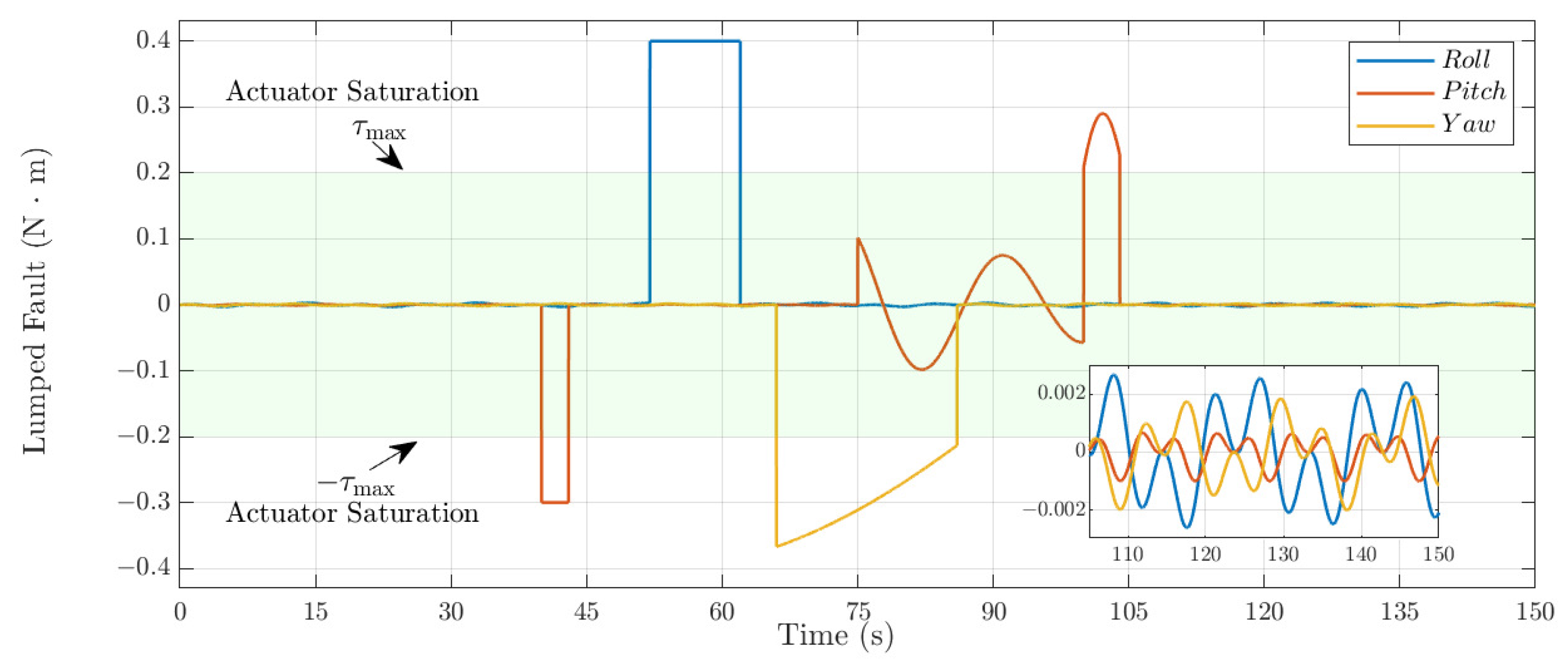
The lumped $\mathit{f}$ is obtained by induction as in (6), and the relationship between $\mathit{f}$ and actuator saturation is intuitively shown in Figure 5. The green coverage area in the figure represents the available output of the actuator, that is, $[-0.2,0.2]$ N·m. It is not difficult to see that the fault scenarios given in Table 2 obviously exceed the ${\tau }_{max}$, in order to verify the resilience and fault tolerance of ARPPC to large-scale faults. The overall simulation time is set as 150 s with a time step of 0.01 s. The design parameters of the relevant control law based on ARPC and the parameter selection of CES are given in

Table 3. Parameter selection.

Parameters	Value
ARPC Envelope	$k=0.1,b=0.9,{\rho }_0=0.1,{\rho }_{\infty }=0.0001$
	$t_f=[40,30,60]$
	${\delta }_1=1,{\delta }_2=0.5,{\delta }_3=0.17$
	$\lambda =3,\nu =0.4,{\kappa }_1=0.1,{\kappa }_2=1$
Control Law	$k_1=0.02,k_2=0.3,k_3=0.18$
	$p=3,q=5,\chi =0.6,\zeta =0.001$
CES	$m=3,z=2$
	$o_0^1=0.03,o_1^1=0.037,o_2^1=0.048,o_3^1=0.056$
	$o_0^2=0.02,o_1^2=0.024,o_2^2=0.033,o_3^2=0.047$
	$o_0^3=0.02,o_1^3=0.022,o_2^3=0.032,o_3^3=0.040$

.

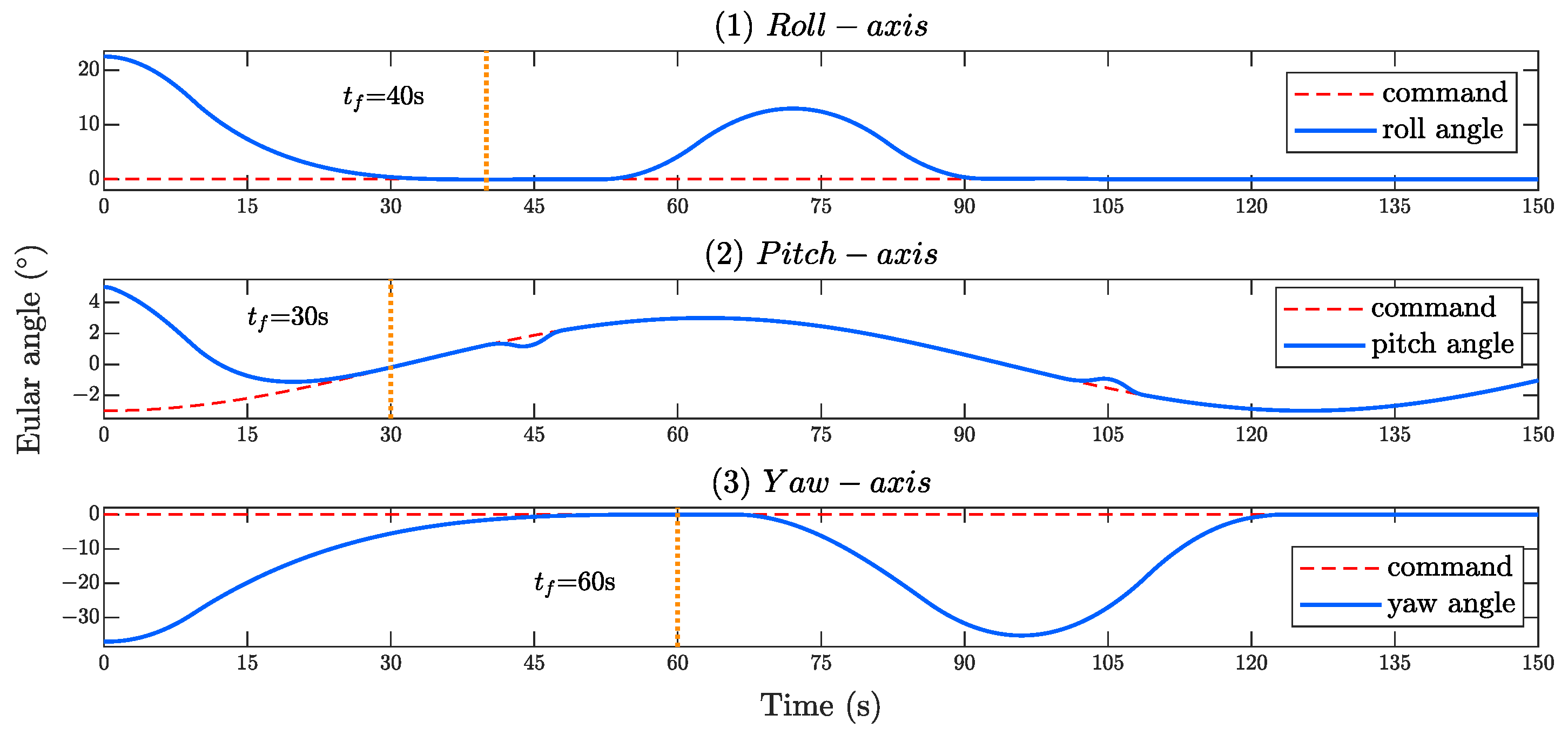
In order to clearly and intuitively show the attitude changes of the spacecraft under the proposed fault-tolerant control law based on ARPC and CES, Figure 6 shows the three-axis attitude angle time response described by the Euler angle. The red dotted line represents the desired attitude maneuver trajectory, and the blue solid line represents the Euler angle time response under the ARPC. It can be seen that the attitude can converge to the desired trajectory within the specified convergence time $t>t_f$. When $t>t_f$ enters the steady-state stage, corresponding to Figure 7, the Euler angle can still be within the performance envelope under faults or disturbances exceeding the saturation level and finally reconverge to the desired trajectory. This proves the adaptability and robustness of the ARPC proposed in this paper from another perspective.

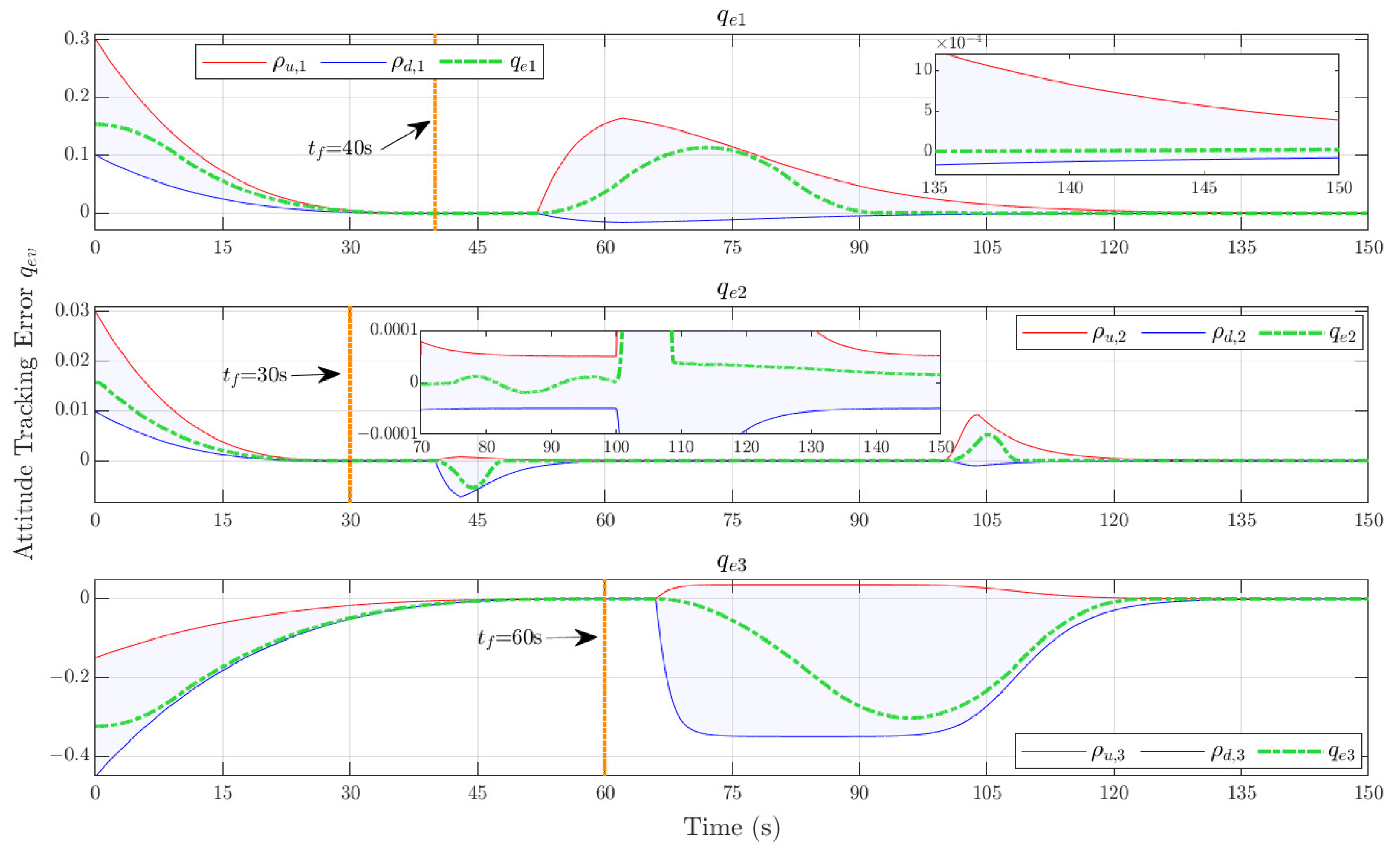
Figure 7 demonstrates the response of the spacecraft attitude under the fault-tolerant control law based on ARPC and CES proposed in this paper. The three sub-figures respectively demonstrate the response of $q_{e1}\left(t\right),q_{e2}\left(t\right),q_{e3}\left(t\right)$, and the red and blue solid lines represent the upper boundary ${\rho }_{u,i}\left(t\right)$ and lower boundary ${\rho }_{d,i}\left(t\right)$ of the adhesive-resilient prescribed performance envelope respectively. The green dotted line represents the error quaternion $q_{e,i}\left(t\right)$.

First, it can be seen from Figure 7 that under the same initial envelope ${\rho }_0$, through the automatic correction of the initial adhesive mechanism ${\phi }_1\left(t\right),{\phi }_2\left(t\right)$, the initial envelopes of the three axes of roll, pitch, and yaw are adjusted according to different initial errors, and $q_{e,i}\left(0\right)$ is accurately captured to the new performance envelope, thereby avoiding the control singularity caused by the error falling outside the envelope. At the same time, the automatic correction of the initial adhesive mechanism ${\phi }_1\left(t\right),{\phi }_2\left(t\right)$ also ensures that there is no overshoot in the transient performance constraint, constrains the attitude error with a narrower and more precise performance envelope, and improves the performance of the controller.

Furthermore, through the proposed fault-tolerant control law, the error $q_{e,i}\left(0\right)$ can converge to the steady-state performance range within the appointed time specified by the user. It can always ensure that ${\rho }_d\left(t\right)<q_{ei}\left(t\right)<{\rho }_u\left(t\right),i=1,2,3$ is satisfied. Corresponding to the fault in Figure 5, it is not difficult to see that due to the limitation of ACS actuator saturation, the error will inevitably increase when facing the above-mentioned faults or disturbances exceeding the saturation level. At this time, ARPC can actively relax the performance envelope in advance, temporarily allowing the error to deviate from the ideal steady-state accuracy, and give priority to ensuring the stability of the prescribed performance control. Wait until the fault or disturbance is weakened to the range that the actuator can fully compensate, and then tighten the performance envelope again to achieve higher control accuracy. While solving the robustness and static problems of the prescribed performance control, the conservatism of the controller is greatly reduced. Thanks to the intervention of prescribed performance control, the accuracy of attitude tracking control can reach $0.{0008}^{\circ }$ after entering the steady-state stage. At the same time, it can ensure excellent control stability.

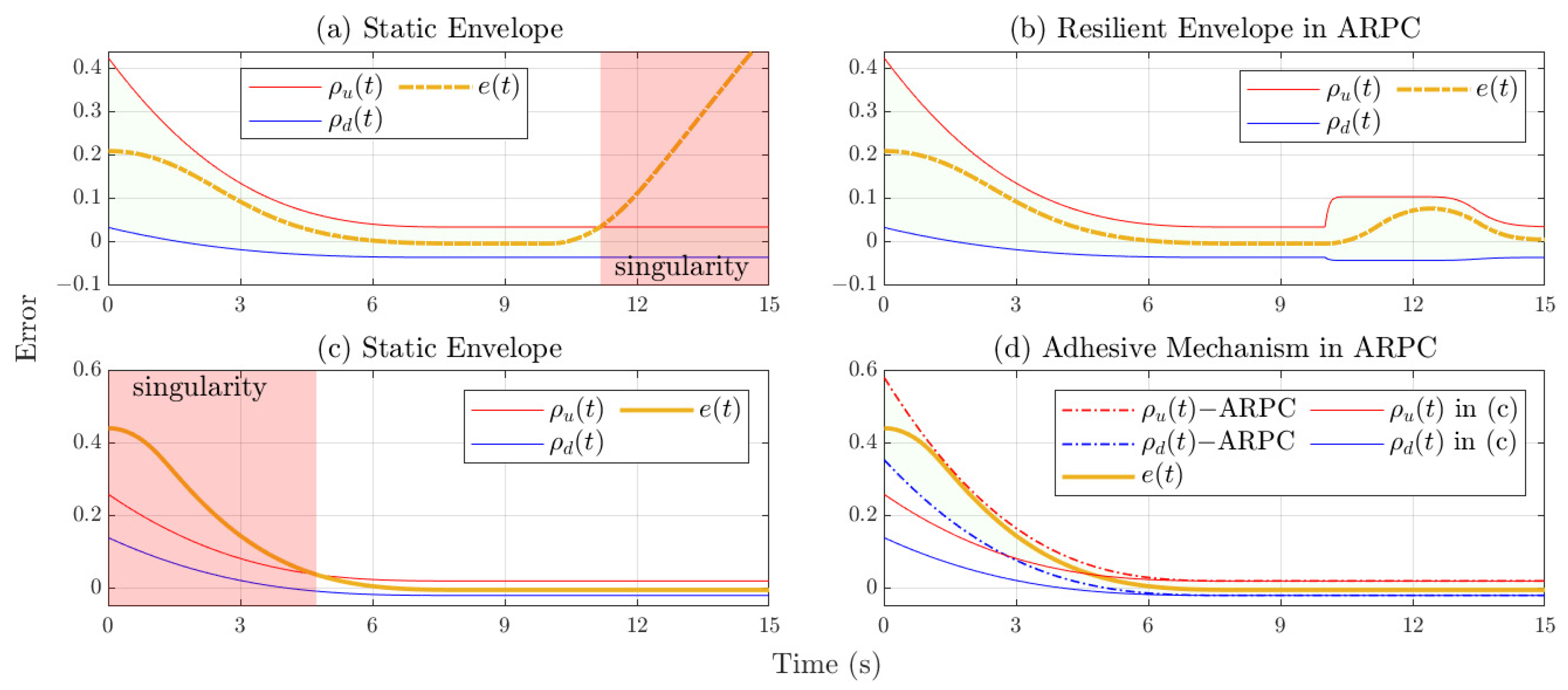
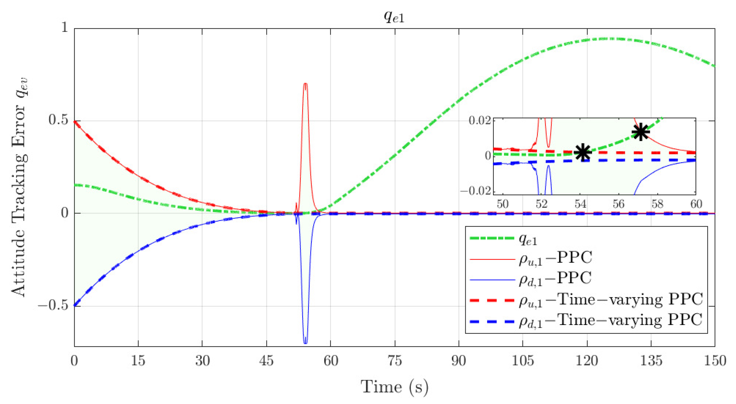
To verify the superiority of the proposed method, Figure 8 shows the results of applying the existing methods to the same fault scenarios in this section. The blue and red dashed lines represent the traditional PPC lower and upper boundaries in [14]. The blue and red solid lines represent the improved time-varying PPC lower and upper boundaries in [19]. As demonstrated in the figure, “∗” means that the error exceeds the inherent performance envelope and it makes the control design suffer from the singularity problem.

It is not difficult to see that the traditional PPC does not have the ability to perform online adaptive adjustment because it is a static function. Therefore, when encountering the same large-scale fault or disturbance, the tracking error will quickly exceed the inherent static envelope, thereby inducing control singularity. Although [19] provides a mechanism for online correction of PPC based on the error change trend, it only considers the accumulation of errors and does not consider that large-scale faults will induce actuator saturation. This makes it difficult for its online adjustment speed to catch up with the accumulation speed of tracking errors, and the problem of control singularity still exists. In contrast, the method proposed in this paper can generate the resilient performance envelope more accurately by comprehensively evaluating the changing trend of the tracking error and the saturation degree of the actuator and is therefore more effective in dealing with large-scale faults or disturbances.

On the other hand, the method in Figure 8 cannot achieve convergence within an appointed time, which makes it impossible to constrain transient performance more accurately according to the desired index. It is not difficult to see that the upper and lower boundaries of the PPC in Figure 8 are symmetrical, which has the disadvantage of being unfavorable for constraining the overshoot. More importantly, the PPC represented by these two methods always exists in the initial performance envelope ${\rho }_0$, which is heavily dependent on the prior information of ${\mathit{q}}_{ev}\left(0\right)$. In other words, when a new control reference is received, the controller needs to re-initialize the parameters of ${\rho }_0$ according to the new ${\mathit{q}}_{ev}\left(0\right)$. There is no set of regular adjustment methods and it is too dependent on manual experience. As shown in Figure 7, the ARPC proposed in this paper can automatically generate a new initial performance envelope through the adhesive mechanism in (12), avoiding the above problem.

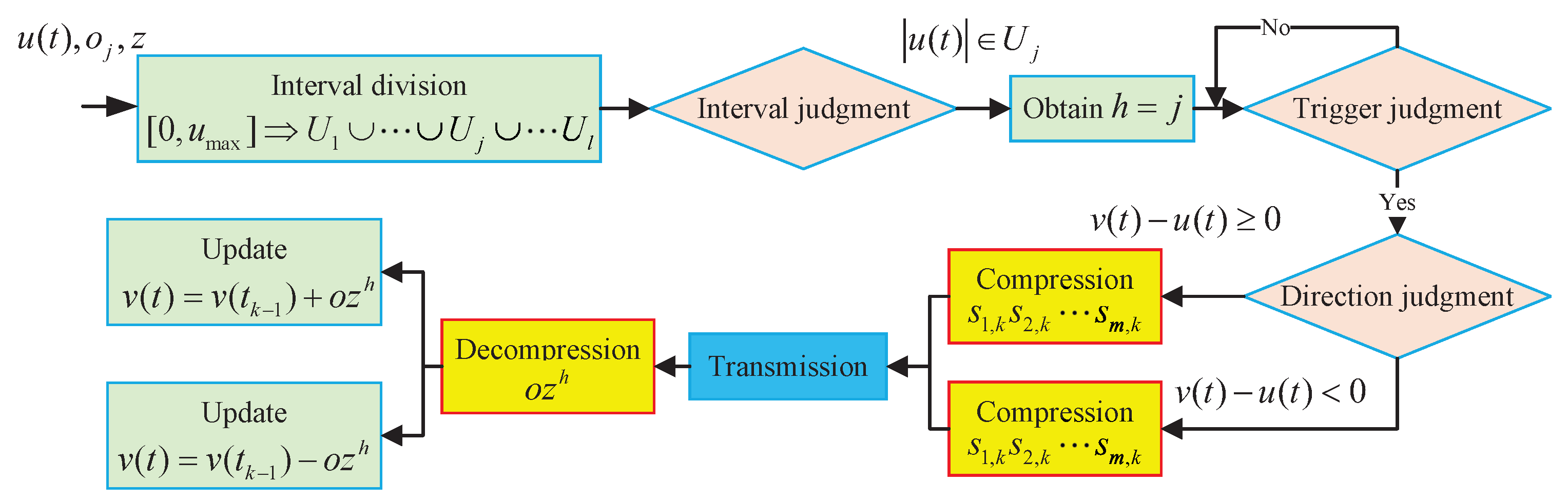
Figure 9 demonstrates the control torque $v_a\left(t\right)$ response of the fault-tolerant control law under the CES update strategy. It can be clearly seen that after the transformation of the CES update strategy, the output torque becomes a step-change response. However, it is worth noting that, unlike the fixed threshold event-trigger mechanism in [28,29], the step change is not a fixed increment, but an adaptive increment automatically generated by measuring and compression according to the control input size. This dynamic threshold facilitates more accurate tracking performance and ensures fast response to signal changes when $u\left(t\right)$ is large through a constant threshold. Also different from the relative threshold event-trigger mechanism [26], which is always monotonically increasing, CES can strike a good balance between avoiding signal distortion and dynamic performance.

To further demonstrate the advantages of CES, Figure 10 shows the trigger levels recorded by the trigger mechanism at different times. Among them, “No Trigger” means that the actuator does not need to be updated; that is, no data are transmitted between the control box and the actuator at this time. “Level 1” to “Level 4” represent higher-level update increments. It is not difficult to see that the higher the level, the fewer the trigger times, and the system is in a non-communication state most of the time. It will only perform transmission based on compression and decompression when necessary to ensure that the tracking error is within the performance envelope.

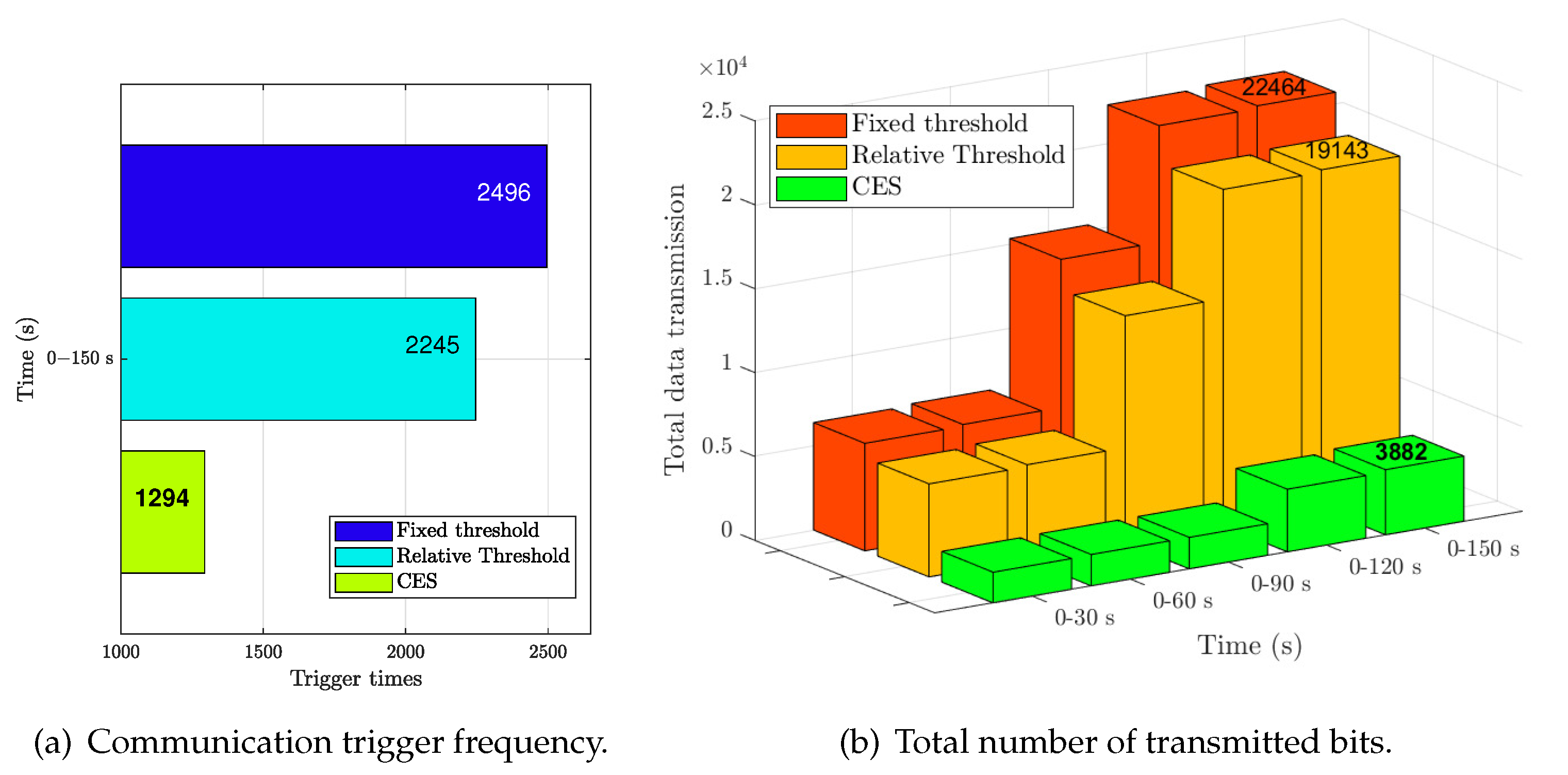
Figure 11a shows the comparison of the number of triggered communications under different event-triggered update strategies, which mainly includes the fixed threshold event trigger mechanism in [28,29], the relative threshold event trigger mechanism in [26] and CET in this paper. It is clear from Figure 11a that the proposed CES update strategy reduces the frequency of communication compared to other methods. Note that CES and z-ary compression transmission accomplish a good balance between tracking performance and network constraints. In order to further demonstrate the impact of different $z,m$ values and coefficient o selection on CES performance, a brief comparison is made here for the scenario when $z=6,m=4$. At this time, the communication trigger frequency will increase sharply to 2128. The total number of transmitted bits will also increase synchronously to 12,768. This is due to the increase of $z,m$. The number of intervals l that divide $u\left(t\right)$ also increases accordingly, which leads to more refined and easier to achieve trigger condition judgment. The increase of m directly means that the number of bytes transmitted in a single transmission increases, which will inevitably lead to the increase of the total number of bits transmitted. There is no fixed rule for the selection of coefficient o. Generally speaking, a larger o means that the trigger condition is more difficult to achieve, which will reduce the number of triggers. However, it also means more precision loss. The selection of o should be further weighed according to the required control performance and communication resources.

In addition, the total amount of overall control signal data transmission and its comparison are specifically given in Figure 11b. It is obvious that CES requires the least amount of data transmission throughout the control process, and that this is far less than other methods. In contrast, the traditional event trigger mechanism only focuses on reducing the communication frequency, while still transmitting the control signal as original data during the communication process, which will result in a single transmission of a 9-bit or even 12-bit string. In each communication between the control box and the actuator, CES compressed the control input error as a 3-bit string. This means that the total amount of data transmission required during the signal transmission process is greatly reduced. At the same time, since the compression and decompression rules are user-defined, there is only a string of z-ary characters in the communication process. Unlike traditional event-triggered methods, it encodes control signal updates according to a private rule before transmission over the data bus, with the actuator decoding the signal using a predefined decompression rule. Even if it is intercepted, the real control signal cannot be restored due to the lack of decompression rules, effectively preventing data leakage or manipulation. Additionally, by reducing the amount of transmitted data, the scheme lowers communication bandwidth requirements and mitigates the risk of potential data leakage. The dynamic adaptability of the encoding further complicates prediction by attackers, enhancing the overall security of the system. Thus, the proposed method significantly enhances the communication security of spacecraft control systems.

5. Conclusions

This paper develops an adhesive-resilient prescribed control for spacecraft ACS with a z-ary compression event-triggered scheme. The designed ARPC adaptively relaxes or narrows the performance envelope to handle large-scale faults and eliminates dependence on initial conditions. While solving the control singularity, the conservatism and adaptability are significantly improved. The fault-tolerant control law designed effectively compensates for any fault within the framework of the prescribed performance without inducing chattering, ensuring the specified transient performance and steady-state accuracy. Additionally, the z-ary CES is shown to reduce communication frequency and total data transmission by approximately 40% and 70%, respectively, compared with traditional event-triggered methods. This leads to a significant reduction in communication bandwidth consumption while enhancing communication security, as each transmission only compresses and transmits a specific length of bits. In the future, the protocol will be designed based on the changing rate of the control signal to further improve tracking performance.