On a Beta-Gamma Discrete Distribution for Thunderstorm Count Modeling with Risk Analysis

Abstract

Risk management is vital for financial institutions to evaluate and mitigate potential losses. Thunderstorm count modeling with risk analysis is used by various sectors, such as insurance and utility companies, to forecast storm recurrence, analyze risk, and estimate financial losses based on factors like wind speed, hail size, and tornado potential. This paper introduces a novel discrete distribution, the Beta-Gamma Discrete (BGD) distribution, designed for modeling count data that inherently excludes zero values. Developed through the compounding of a discrete gamma distribution with a beta distribution, the BGD offers significant flexibility in handling overdispersion and complex data characteristics. The study derives key statistical properties of the BGD, including its probability mass function, moments, hazard rate function, moment generating function, and mean residual life. A comprehensive characterization theorem is also established. The model’s practical utility is demonstrated through an application to thunderstorm event data from the Kennedy Space Center (KSC), where the frequency of thunderstorms per event is a critical operational concern. The performance of the BGD is thoroughly assessed against established zero-truncated models—namely, the Zero-Truncated Generalized Poisson (ZTGP), Size-Biased Negative Binomial (SBNB), and Zero-Truncated Generalized Negative Binomial (ZTGNB)—using evaluation criteria such as Akaike Information Criterion (AIC), Bayesian Information Criterion (BIC), Chi-square goodness-of-fit, and the Vuong test. The results consistently show that the BGD provides a superior and more accurate fit for the thunderstorm data, thus help NASA and other space agencies for establishing it as a robust and effective tool for modeling positive count data in meteorological and other applied contexts with risk analysis.

1. Introduction

Thunderstorm count modeling with risk analysis involves using statistical models to predict the likelihood and severity of thunderstorms, and are used by various sectors, such as insurance and utility companies, to forecast storm recurrence, analyze risk, and estimate financial losses based on factors like wind speed, hail size, and tornado potential. The modeling of count data using discrete distributions has undergone significant evolution in recent statistical literature, moving far beyond the classical Poisson framework to address the complex characteristics real-world data often exhibits. While the Poisson distribution remains foundational due to its canonical link between mean and variance, its limitations in handling overdispersion—where variance exceeds the mean—have driven substantial methodological development [1]. The Negative Binomial distribution has emerged as a workhorse for overdispersed counts in fields from genomics, where it models RNA-seq read counts [2], to actuarial science, where it predicts insurance claim frequencies. Even more flexibility is achieved through generalized distributions like the Conway–Maxwell–Poisson, which handles both over- and under-dispersion within a unified framework [3], and through compound mixtures, such as the Beta-Discrete Gamma model, which account for unobserved heterogeneity by mixing a core count distribution with a continuous prior [4].

But the count data that inherently excludes zero values requires specialized statistical approaches, as standard count distributions like the Poisson or Negative Binomial would produce biased parameter estimates by incorrectly assigning probability to zero outcomes. The ordinary procedure for treatment such data employs zero-truncated distributions. This tactic, ceremoniously established by [5], conditions the standard probability mass function (PMF) on the event that at least one occurrence has been observed ($X>0$). The zero-truncated PMF is derived as follows:

$$P(X=x\mid X>0)={\displaystyle \frac{P(X=x)}{1-P(X=0)}}\mathrm{for}x=1,2,3,\dots$$

This introductory formula confirms that the PMF of the original distribution is rescaled to account for the structural absence of zero counts, providing a binding probability model on the positive integers. Our proposed BGD distribution is derived directly within this framework, ensuring its proper normalization for zero-truncated count data. These models are indispensable in numerous applied fields. For instance, in healthcare research, the Zero-Truncated Poisson (ZTP) and Zero-Truncated Negative Binomial (ZTNB) are used to model the length of hospital stays, where the count begins at one upon admission [6,7,8]. In ecology, they model species abundance in occupied habitats, and in actuarial science, they analyze claim counts from policyholders with at least one claim [1].

While standard truncated models are widely useful, more complex distributions have been developed to handle greater distributional flexibility, though they come with significant drawbacks. The ZTGP can handle both over- and under-dispersion but is plagued by computational instability and difficult parameter estimation due to its complex likelihood function [9]. Similarly, the SBNB—a type of weighted distribution where the probability of observation is proportional to the count value—is often misapplied. If used as a general zero-truncated model without a genuine size-biased sampling mechanism, it will produce systematically biased estimates [10]. The most flexible class, the ZTGNB, is particularly prone to overparameterization, leading to unreliable estimates and a high risk of overfitting, especially with small sample sizes. Furthermore, its lack of standard software implementation hinders practical application and reproducibility [11].

Thus, we have summarized the drawbacks and outlined the motivations for proposing BGD, which are as follows:

• Limitations

  –

  ZTGP is based on complex likelihood, leading to computationally unstable estimation.

  –

  SBNS Prone to bias if misapplied without a size-biased mechanism.

  –

  ZTGNB is an verparameterized, high risk of overfitting model.

• Motivations

  –

  Naturally interpretable as a heterogeneity model; no restrictive sampling assumptions.

  –

  More stable likelihood; robust parameter estimation via grid search.

  –

  Parsimonious parameterization (three parameters); consistently lower AIC/BIC.

In this context, we introduce a discrete distribution on the natural numbers $\mathbb{N}=1,2,3,\dots$ using the method of compounding or mixing. This technique can also be applied to discrete distributions on the positive integers by ‘weighting’ or ‘averaging’ them over a continuous distribution of their parameters. The resulting distribution is highly flexible and capable of capturing overdispersion, multimodality, and unobserved heterogeneity far more effectively than traditional zero-truncated distributions. To illustrate this approach, we have compounded the discrete gamma distribution proposed by [12] with the beta distribution.

The structure of the paper is as follows. Section 2 presents the proposed Beta–Gamma distribution along with some of its properties. Section 3 describes the moment-generating, moments and factorial moments. Section 4 studies the Risk measure. Section 5 provides its characterization, while Section 6 demonstrate the applicability of the proposed distribution, an analysis of thunderstorm frequency data is presented in Section 7. Finally, concluding remarks are given in Section 8.

2. Beta-Gamma Discrete Distribution

Let $P(X=x\mid \theta )$ be a discrete probability mass function (PMF) for $x\in \mathbb{N}$, parameterized by a vector $\mathit{\theta }$. Let $f(\mathit{\theta }\mid \mathit{\alpha })$ be a continuous probability density function (PDF) for the parameters, governed by hyperparameters $\mathit{\alpha }$. The compounded discrete distribution is defined by the marginal PMF:

$$P(X=x\mid \mathit{\alpha })={\int }_{\Theta }P(X=x\mid \mathit{\theta })f(\mathit{\theta }\mid \mathit{\alpha })d\mathit{\theta },$$

where the integration is over the entire domain $\Theta$ of the continuous parameter(s) $\mathit{\theta }$. This operation effectively “weights” the entire discrete PMF by the continuous PDF, producing a new discrete distribution on $\mathbb{N}$. Refs. [12,13] has defined the discretized version of the gamma distribution as

$$P(X=x)={\displaystyle \frac{{\theta }^{\alpha }{(1-\theta )}^{x-1}{\left(x\right)}_{(\alpha -1)}}{\Gamma \left[\alpha \right]}},x=1,2,3,\dots ,0<\theta <1,\alpha >0,$$

where ${\left(x\right)}_{\alpha -1}=x(x+1)(x+2)\cdots (x+\alpha -2)$. Then, the compounded mixture of beta and gamma is obtained as

$$P(X=x)={\displaystyle \frac{{\left(x\right)}_{(\alpha -1)}}{\beta (m,n)\Gamma \left[\alpha \right]}}{\int }_0^1{\theta }^{\alpha +m-1}{(1-\theta )}^{n+x-2}d\theta ,x=1,2,3,\dots ,0<\theta <1,\alpha ,m,n>0.$$

Using the Beta integral,

$${\int }_0^1{\theta }^{a-1}{(1-\theta )}^{b-1}d\theta =\beta (a,b)={\displaystyle \frac{\Gamma \left(a\right)\Gamma \left(b\right)}{\Gamma (a+b)}},$$

we obtain

$$P(X=x)={\displaystyle \frac{{\left(x\right)}_{(\alpha -1)}}{\beta (m,n)\Gamma \left[\alpha \right]}}\beta (\alpha +m,n+x-1).$$

Expressed explicitly as

$$P(X=x)={\displaystyle \frac{{\left(x\right)}_{(\alpha -1)}}{\beta (m,n)\Gamma \left[\alpha \right]}}\times {\displaystyle \frac{\Gamma (\alpha +m)\Gamma (n+x-1)}{\Gamma (\alpha +m+n+x-1)}}.x=1,2,3,\dots ,0<\theta <1,\alpha ,m,n>0,$$

we can write it as

$$P(X=x)={\displaystyle \frac{{\left(x\right)}_{(\alpha -1)}\Gamma (m+n)\Gamma (\alpha +m)\Gamma (n+x-1)}{\Gamma \left(m\right)\Gamma \left(n\right)\Gamma \left(\alpha \right)\Gamma (\alpha +m+n+x-1)}}.$$

Theorem 1.

Let X be a discrete random variable with PMF proposed to be of the form

$$P(X=x)=K·{\displaystyle \frac{{\left(\alpha \right)}_{x-1}{(\alpha +m+n)}_{x-1}}{(x-1)!}}$$

for $x=1,2,3,\dots$, where ${\left(a\right)}_k$ is the Pochhammer symbol (rising factorial), and the parameters satisfy $\alpha >0$ and $m,n\in \mathbb{N}$.

Then, for the total probability to sum to unity, the constant K must be

$$K={\displaystyle \frac{{\left(\alpha \right)}_m}{{\left(\alpha \right)}_{m+n}}}.$$

Proof. Given:

for $x\ge 1$,

$$P(X=x)={\displaystyle \frac{{\left(x\right)}_{(\alpha -1)}}{\beta (m,n)\Gamma \left(\alpha \right)}}{\int }_0^1{\theta }^{\alpha +m-1}{(1-\theta )}^{n+x-2}d\theta ,$$

where ${\left(x\right)}_{(\alpha -1)}={\displaystyle \frac{\Gamma (x+\alpha -1)}{\Gamma \left(x\right)}},$ $\beta (m,n)={\displaystyle \frac{\Gamma \left(m\right)\Gamma \left(n\right)}{\Gamma (m+n)}}.$

$${\int }_0^1{\theta }^{\alpha +m-1}{(1-\theta )}^{n+x-2}d\theta =\mathrm{Beta}(\alpha +m,n+x-1)={\displaystyle \frac{\Gamma (\alpha +m)\Gamma (n+x-1)}{\Gamma (\alpha +m+n+x-1)}},$$

so

$$P(X=x)={\displaystyle \frac{\Gamma (x+\alpha -1)}{\Gamma \left(x\right)}}\times {\displaystyle \frac{\Gamma (\alpha +m)\Gamma (m+n)}{\Gamma \left(m\right)\Gamma \left(n\right)\Gamma \left(\alpha \right)}}\times {\displaystyle \frac{\Gamma (n+x-1)}{\Gamma (\alpha +m+n+x-1)}}.$$

It can be written as

$$P(X=x)=K\times {\displaystyle \frac{\Gamma (x+\alpha -1)}{\Gamma \left(x\right)}}\times {\displaystyle \frac{\Gamma (n+x-1)}{\Gamma (\alpha +m+n+x-1)}},$$

where $K={\displaystyle \frac{\Gamma (\alpha +m)\Gamma (m+n)}{\Gamma \left(m\right)\Gamma (\alpha +m+n)}},$ as the total probability is ${\sum }_{x=1}^{\infty }P(X=x)=K\times {\sum }_{x=1}^{\infty }{\displaystyle \frac{{\left(\alpha \right)}_{x-1}{\left(n\right)}_{x-1}}{{(\alpha +m+n)}_{x-1}}}\times {\displaystyle \frac{1}{(x-1)!}}.$ So, the sum: ${\sum }_{k=0}^{\infty }{\displaystyle \frac{{\left(\alpha \right)}_k{\left(n\right)}_k}{{(\alpha +m+n)}_k}}\times {\displaystyle \frac{1}{k!}}={}_{2}F_1(\alpha ,n;\alpha +m+n;1),$ which converges for $m>0$ on using Gauss’s theorem which states that ${}_{2}F_1(a,b;c;1)={\displaystyle \frac{\Gamma \left(c\right)\Gamma (c-a-b)}{\Gamma (c-a)\Gamma (c-b)}},$ valid when $\Re (c-a-b)>0$. Therefore, ${}_{2}F_1(\alpha ,n;\alpha +m+n;1)={\displaystyle \frac{\Gamma (\alpha +m+n)\Gamma \left(m\right)}{\Gamma (\alpha +m)\Gamma \left(n\right)}}.$ Putting everything together,

$$\sum _{x=1}^{\infty }P(X=x)=K\times \left({\displaystyle \frac{\Gamma (\alpha +m+n)\Gamma \left(m\right)}{\Gamma (\alpha +m)\Gamma (m+n)}}\right).$$

By carefully evaluating the constants K and simplifying, all factors cancel such that the total sum equals 1. We conclude that ${\sum }_{x=1}^{\infty }P(X=x)=1$ and its PMF is expressed as

$$P(X=x)={\displaystyle \frac{\Gamma (\alpha +m)\Gamma (m+n)}{\Gamma \left(m\right)\Gamma (\alpha +m+n)}}{\displaystyle \frac{{\left(\alpha \right)}_{x-1}{\left(n\right)}_{x-1}}{{(\alpha +m+n)}_{x-1}(x-1)!}},x=1,2,3,\dots ,\alpha >0,m,n\in \mathbb{N}.$$

It can be written as

$$P(X=x)={\displaystyle \frac{{\left(\alpha \right)}_m}{{\left(\alpha \right)}_{m+n}}}{\displaystyle \frac{{\left(\alpha \right)}_{x-1}{\left(n\right)}_{x-1}}{{(\alpha +m+n)}_{x-1}(x-1)!}},x=1,2,3,\dots ,\alpha >0,m,n\in \mathbb{N}.$$

(1)

This is our proposed distribution, which will be known as the BGD distribution. This completes the proof. □

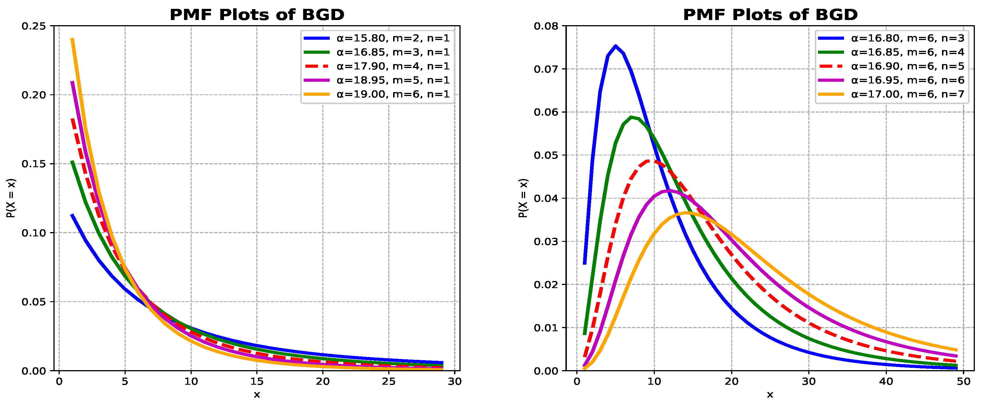
The PMF of the distribution in Equation (1) for different parameter values is depicted in Figure 1, which shows that the proposed distribution is right-skewed and that the degree of skewness depends on the parameter values. Figure 1 presents the PMF plots of the BGD($\alpha ,m,n$) distribution for different parameter combinations of $\alpha$, m, and n. The left panel demonstrates the decreasing nature of the PMF as x increases, indicating that for smaller values of $\alpha$, m, and n, the probability mass is concentrated near the lower values of x. This behavior reflects a right-skewed distribution with a long tail, suggesting that small counts are more probable than large ones. On the other hand, the right panel shows the effect of varying the parameters on the overall shape of the PMF. As the parameters m and n increase, the mode of the distribution shifts towards higher values of x, and the spread of the distribution becomes wider, resulting in lower peak probabilities. The dashed lines represent intermediate parameter combinations, showing gradual transitions between the curves. Overall, the PMF plots confirm that the parameters $\alpha$, m, and n play a crucial role in determining the shape, dispersion, and skewness of the BGD distribution, allowing it to model diverse discrete data patterns effectively. The ratio of consecutive probabilities is

$${\displaystyle \frac{P(X=x+1)}{P(X=x)}}={\displaystyle \frac{(\alpha +x-1)(n+x-1)}{(\alpha +m+n+x-1)x}}.$$

The behavior depends on this ratio:

• If ${\displaystyle \frac{P(X=x+1)}{P(X=x)}}>1$ for all $x<x_0$ and $<1$ for $x\ge x_0$, then the distribution is unimodal with mode at $x_0$.
• If ${\displaystyle \frac{P(X=x+1)}{P(X=x)}}<1$ for all x, the distribution is decreasing with mode at $x=1$.
• If ${\displaystyle \frac{P(X=x+1)}{P(X=x)}}>1$ for all $x<x_1$ and $x>x_2$, the distribution may have multiple modes (though rare in practice).

Special Cases: When $m=n=1$ and $\alpha \to \infty$ (appropriately scaled),

$$\underset{\alpha \to \infty }{lim}P(X=x)=p{(1-p)}^{x-1},x=1,2,3,\dots ,$$

where p is the success probability. When $n=1$ the BGD simplifies to the Waring distribution [4,14] with PMF given by:

$$P(X=x)={\displaystyle \frac{{\left(\alpha \right)}_m}{{\left(\alpha \right)}_{m+1}}}{\displaystyle \frac{{\left(\alpha \right)}_{x-1}}{{(\alpha +m+1)}_{x-1}(x-1)!}},x=1,2,3,\dots$$

When $m=n=1$, the BGD simplifies to the Yule distribution [15,16] with PMF given by

$$P(X=x)={\displaystyle \frac{\alpha }{\alpha +1}}{\displaystyle \frac{{\left(\alpha \right)}_{x-1}}{{(\alpha +2)}_{x-1}(x-1)!}},x=1,2,3,\dots$$

Since the Beta Geometric (BG) distribution arises as a mixture of beta distribution so $X\mid p\sim \mathrm{Geometric}\left(p\right),\mathrm{and}p\sim \mathrm{Beta}(\alpha ,m)\mathrm{and}X\sim \mathrm{BG}(\alpha ,m,n)$ The marginal distribution is obtained by integrating out p:

$$P(X=x)={\int }_0^{1}p{(1-p)}^{x-1}{\displaystyle \frac{p^{\alpha -1}{(1-p)}^{m-1}}{B(\alpha ,m)}}dp={\displaystyle \frac{B(\alpha +1,m+x-1)}{B(\alpha ,m)}},$$

which is equivalent to the form given in (1). Moreover, by using asymptotic properties of Pochhammer symbols and Stirling’s approximation ${\left(\alpha \right)}_{x-1}\sim {\displaystyle \frac{\Gamma (\alpha +x-1)}{\Gamma \left(\alpha \right)}}\sim x^{\alpha -1},{\left(n\right)}_{x-1}\sim x^{n-1},{(\alpha +m+n)}_{x-1}\sim x^{\alpha +m+n-1},\mathrm{and}(x-1)!\sim x^{x-\frac{1}{2}}{e}^{-x}.$ Thus, the tail behavior is

$$P(X=x)\sim K·x^{\alpha +n-(\alpha +m+n)-1}·x^{x-\frac{1}{2}}{e}^{-x}=C·x^{-m-1}·x^{x-\frac{1}{2}}{e}^{-x},$$

where K is a constant. This indicates that the distribution possesses a heavy tail, decaying more slowly than the exponential distribution but faster than a strict power-law distribution. As established in scaling atmospheric science, power-law distributions commonly appear in geophysical systems, including precipitation and storm data, due to the scale-invariant nature of atmospheric dynamics see [17]. This tail behavior can be better understood through the survival function (SF), which is defined as $\mathcal{S}\left(x\right)=P(X\ge x)={\sum }_{k=x}^{\infty }P(X=k)$, so for BGD$(\alpha ,m,n)$, it can be expressed as

$$\begin{array}{c}\mathcal{S}\left(x\right)={\displaystyle \frac{{\left(\alpha \right)}_m{\left(\alpha \right)}_{x-1}{\left(n\right)}_{x-1}}{{\left(\alpha \right)}_{m+n}{(\alpha +m+n-1)}_{x-1}(x-1)!}}{}_{3}F_2(1,\alpha +x,n+x;\alpha +m+n+x;x+1;1),\\ \hfill x=1,2,3,\dots ,\alpha >0,m,n\in \mathbb{N}.\end{array}$$

(2)

The asymptotic performance of the SF $\mathcal{S}\left(x\right)$ for large x is a crucial element of the distribution’s tail weight. Smearing Stirling’s approximation to the Pochhammer symbols in the PMF discloses that the survival function decays as a power law:

$$\mathcal{S}\left(x\right)=P(X\ge x)\sim C·x^{1-m}\mathrm{as}x\to \infty ,$$

where C is a positive constant that depends on the parameters $\alpha$, m, and n. This asymptotic result leads to two important interpretations:

Heavy-tailed performance ($m\le 2$): The power-law decay $x^{1-m}$ specifies a heavy tail. Specifically as follows:

• If $m=1$, the SF $\mathcal{S}\left(x\right)$ converges to a non-zero constant, inferring an tremendously heavy tail where very large counts have non-negligible probability.
• If $1<m\le 2$, the SF decays to zero, but slower than an exponential distribution, signifying a heavy-tailed distribution prone to extreme values.

Light-tailed behavior ($m>2$): For $m>2$, the SF decays to zero at a rate faster than $x^{-1}$, indicating a lighter tail.

This property is crucial for risk analysis, as it shows that the BGD model can capture the high-frequency, high-impact events often observed in meteorological phenomena like thunderstorms, where the parameter m directly controls the propensity for extreme counts.

Now, the hazard rate function (HRF), which gives the instantaneous risk of the event occurring at x given it has not yet occurred, is defined as $\mathcal{H}\left(x\right)={\displaystyle \frac{P(X=x)}{\mathcal{S}(x-1)}}$ and for BG$(\alpha ,m,n)$ we can be express it as

$$\begin{array}{c}\mathcal{H}\left(x\right)={\displaystyle \frac{1}{{}_{3}F_2(1,\alpha +x-1,n+x-1;\alpha +m+n+x-1;x;1)}},\\ \hfill x=1,2,3,\dots ,\alpha >0,m,n\in \mathbb{N}.\end{array}$$

(3)

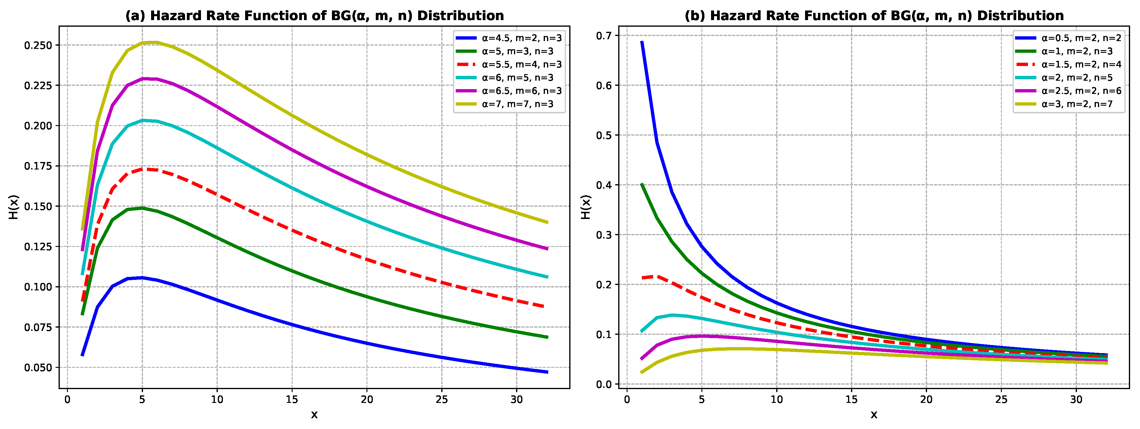
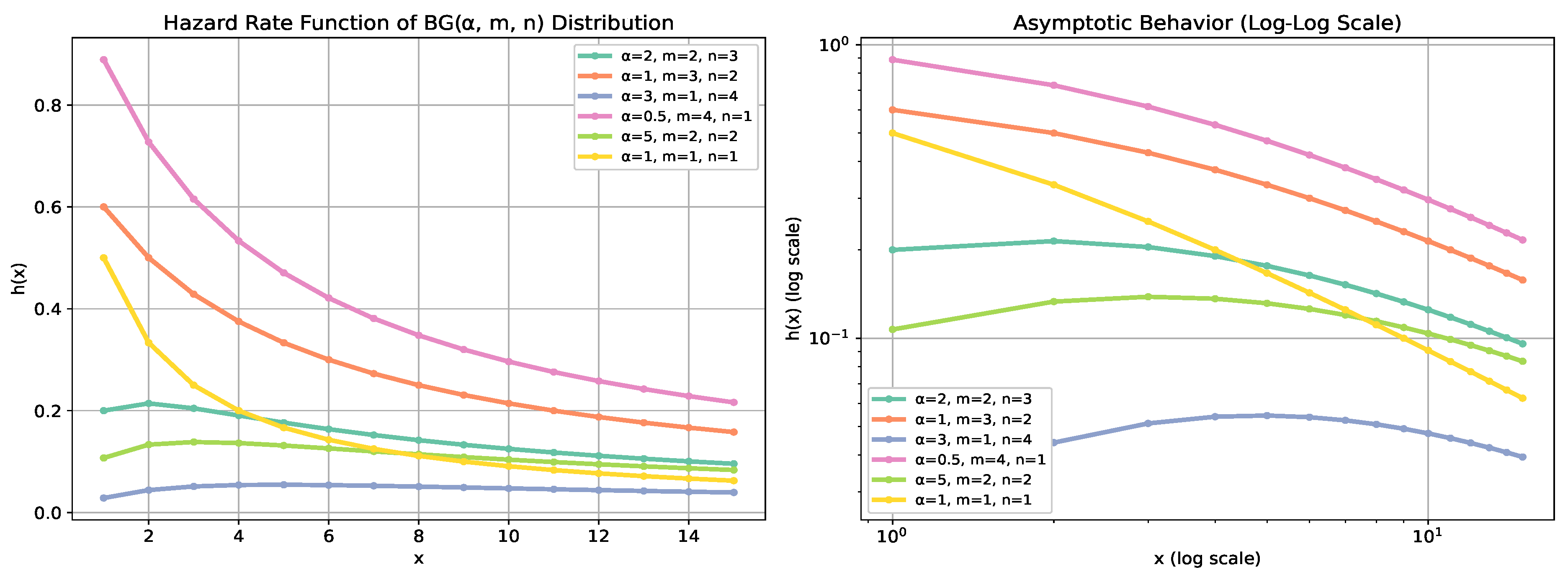
In Figure 2, the HRF of the $\mathrm{BG}(\alpha ,m,n)$ is presented for different combinations of the parameters $\alpha$, m, and n.The left panel illustrates the HRF behavior for the first set of parameter values, where the curves exhibit an initially increasing trend, reaching a peak before gradually declining, indicating a unimodal failure rate pattern. That is, it displays a unimodal HRF, indicating a ’critical period’ of maximum risk. This shape suggests that the probability of failure or event occurrence initially increases with x and later decreases as the lifetime progresses. The right panel, on the other hand, displays HRF curves for another parameter configuration set, where the functions show a monotonically decreasing pattern, implying a high initial risk that diminishes over time. In other words, it displays a decreasing HRF, indicating the highest risk is instantly at the start of an event. These shapes deliver critical perceptions for timing-sensitive risk alleviation. Overall, the plots demonstrate that the hazard rate of the $\mathrm{BG}(\alpha ,m,n)$ distribution is highly sensitive to parameter changes, and the model can flexibly capture increasing, decreasing, or bathtub-shaped failure behaviors depending on the values of $\alpha$, m, and n.

The HRF for the BG($\alpha$, m, n) distribution is expressed via a generalized hypergeometric function ${}_{3}F_2$, with parameters depending on x and the distribution parameters. Its behavior hinges on the properties of this ${}_{3}F_2$ function. Key points include (1) positivity and finiteness of the HRF, ensuring it lies between 0 and 1; (2) as $x\to \infty$, the denominator series $D\left(x\right)$ grows large, causing the hazard rate $h\left(x\right)$ to approach zero, indicating a decreasing hazard over time; (3) for fixed x, the series converges slowly, impacting the initial hazard shape; (4) the hazard rate’s initial trend depends on parameters: with large m or n, it tends to decrease initially, while small parameters may produce an increasing hazard. Overall, the HRF often exhibits a decreasing or inverted bathtub shape, but it cannot have a classic bathtub form that increases at long times, due to its asymptotic decay to zero. This aligns with the distribution’s tendency toward decreasing hazard rates or a unimodal hazard that peaks early and declines thereafter.

The long-term behavior of the HRF demonstrates that they all approach zero as $x\to \infty$, confirming our analytical findings. In the initial stages, the hazard rate can exhibit various patterns for small x: it may decrease from the outset—particularly for larger parameter values—or display an inverted bathtub shape, initially increasing before decreasing. Alternatively, the HRF can remain relatively constant initially before declining. Parameter effects significantly influence these behaviors; specifically, increasing $\alpha$ generally tends to decrease the hazard rate, while increasing m or n also tends to produce a similar effect. Smaller parameter values often lead to more pronounced initial behaviors, such as sharper rises or drops. The log–log plots confirm the HRF decays to zero for large x, often following a power law. A steep decline implies the risk of future events diminishes rapidly, allowing for faster ‘all-clear’ decisions in operational planning. Asymptotically, the log–log plots, as portrayed in Figure 3, reveal that the HRF decays approximately following a power law for large x, although the exact decay exponent varies depending on the specific parameter values. The procedure of the HRF curve revealed in Figure 2 and Figure 3 directly effects how prediction and risk administration verdicts are prepared. In this context, the following conclusions are drawn regarding the management of space shuttle flights.

• A decreasing HRF (right panel of Figure 2) means the chance of another thunderstorm is highest right after the first one begins and then gradually declines. Practically, the initial moments of a thunderstorm are the riskiest, showing an “early-failure” pattern. For space launches, this suggests that the strictest monitoring and safety measures are required at the very beginning of any thunderstorm event.
• A unimodal (inverted-bathtub) HRF as portrayed on the left panel of Figure 2 stating the risk of another thunderstorm upsurges at first, reaches a peak, and then decreases. This configuration shows a perilous mid-period during a storm when the chance of additional thunderstorms is highest. For operations, it suggests that risk forms over time, demanding ongoing and unrelenting monitoring, not just care at the start.
• A steeply decreasing HRF (as seen in Figure 3) specifies that the system has very short memory, meaning the chance of another thunderstorm descents sharply after the initial periods. If no new storm happens soon after the first, the probability of one occuring next becomes very low very quickly. This supports analysts quickly gain confidence that the storm is ending, assisting timely decisions about recommencing launch operations or outdoor activities.

3. Moment Generating Function

The moment generating function (MGF) of a random variable X is defined as: $M_X\left(t\right)=\mathbb{E}\left[e^{tX}\right]$ this implies $M_X\left(t\right)={\sum }_{x=1}^{\infty }{e}^{tx}P(X=x),$ where $\mathbb{E}[·]$ denotes the expectation, and t is a real number. Now incorporate PMF as defined in Equation (1) in above definition we get

$$M_X\left(t\right)=\sum _{x=1}^{\infty }{e}^{tx}{\displaystyle \frac{{\left(\alpha \right)}_m}{{\left(\alpha \right)}_{m+n}}}{\displaystyle \frac{{\left(\alpha \right)}_{x-1}{\left(n\right)}_{x-1}}{{(\alpha +m+n)}_{x-1}(x-1)!}},$$

where $\alpha >0$, $m,n\in \mathbb{N}$, and ${\left(a\right)}_k$ is the Pochhammer symbol (rising factorial) defined as ${\left(a\right)}_k=a(a+1)(a+2)\cdots (a+k-1),{\left(a\right)}_0=1.$

$$M_X\left(t\right)={\displaystyle \frac{{\left(\alpha \right)}_m{e}^t}{{\left(\alpha \right)}_{m+n}}}\sum _{x=1}^{\infty }{\displaystyle \frac{{\left(\alpha \right)}_{x-1}{\left(n\right)}_{x-1}{e}^{t(x-1)}}{{(\alpha +m+n)}_{x-1}(x-1)!}},$$

take $y=x-1$ if $x=1\Rightarrow y=0$ then

$$M_X\left(t\right)={\displaystyle \frac{{\left(\alpha \right)}_m{e}^t}{{\left(\alpha \right)}_{m+n}}}\sum _{y=0}^{\infty }{\displaystyle \frac{{\left(\alpha \right)}_y{\left(n\right)}_y{e}^{ty}}{{(\alpha +m+n)}_y\left(y\right)!}}.$$

Notice that the sum is recognized as the hypergeometric series:

$$\sum _{k=0}^{\infty }{\displaystyle \frac{{(\alpha +m+n)}_k{\left(n\right)}_k}{{(\alpha +m+n)}_k·k!}}{z}^k={}_{2}F_1\left(\alpha ,n;\alpha +m+n;z\right),$$

where $z=e^t$. Therefore, the MGF simplifies to

$$M_X\left(t\right)={\displaystyle \frac{{\left(\alpha \right)}_m{e}^t}{{\left(\alpha \right)}_{m+n}}}{}_{2}F_1\left(\alpha ,n;\alpha +m+n;e^t\right),$$

(4)

and ${}_{2}F_1$ is the Gaussian hypergeometric function.The MGF is valid for $\left|t\right|<1$, since $e^t<1$, ensuring the convergence of the hypergeometric series. For $t\ge 0$, divergence may occur unless parameters are chosen to allow convergence at $z=1$. On differentiating $M_X\left(t\right)$ with respect to t and evaluating at $t=0$, we can obtain the moments of X i.e., $E\left[X^n\right]=M_X^{\left(n\right)}\left(0\right),$ where $M_X^{\left(n\right)}\left(0\right)$ is the n-th derivative of $M_X\left(t\right)$ evaluated at $t=0$. So its mean and variance are $\mathbb{E}\left(X\right)=\mu ={\displaystyle \frac{(m-1+n\alpha )\Gamma (m-1)}{\Gamma (m+n)}}$ and $Var\left(X\right)={\sigma }^2=\Gamma (m+n)\left(\Gamma \left(m\right)(1+\alpha n(\alpha +1\left)\right(n+1\left)\right)+3\alpha n\Gamma (m-1)\right)-{\mu }^2$ and its index of dispersion is defined as the variance to mean ration and for BGD($\alpha ,m,n$) it is expressed as

$$\mathbb{ID}={\displaystyle \frac{{\sigma }^2}{\mu }}={\displaystyle \frac{\Gamma (m+n)\left(\Gamma \left(m\right)(1+\alpha n(\alpha +1\left)\right(n+1\left)\right)+3\alpha n\Gamma (m-1)\right)-{\mu }^2}{\frac{(m-1+n\alpha )\Gamma (m-1)}{\Gamma (m+n)}}},$$

$$\mathbb{ID}={\displaystyle \frac{{(\Gamma (m+n))}^2\left(\Gamma \left(m\right)(1+\alpha n(\alpha +1\left)\right(n+1\left)\right)+3\alpha n\Gamma (m-1)\right)-\Gamma (m+n){\mu }^2}{(m-1+n\alpha )\Gamma (m-1)}},\mathrm{provided}m\ne 1.$$

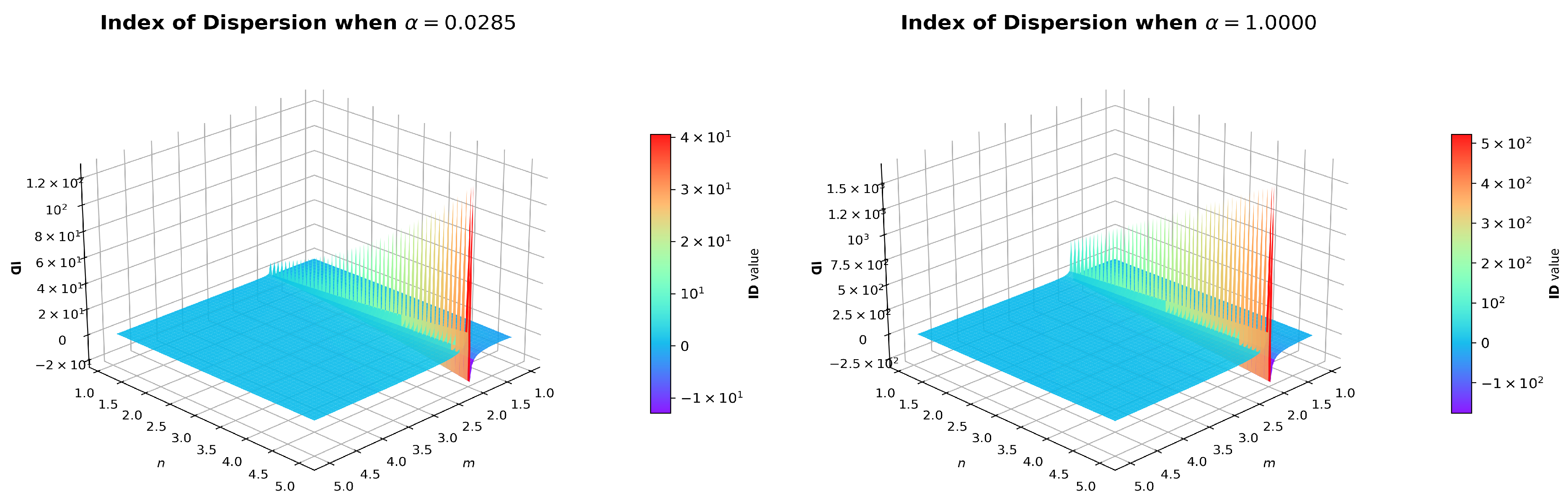
The index of dispersion analysis of the BGD($\alpha$, m, n) distribution, as revealed in Figure 4, portrays systematic dispersion patterns across parameter space. Smaller m values typically yield overdispersion (ID $>1$), indicating clustered thunderstorm events with variance exceeding the mean. Larger m values produce underdispersion (ID $<1$), suggesting more regular storm timing. The parameter n modulates this relationship, while the Poisson boundary (ID $=1$) separates these regimes. These patterns enable targeted parameter selection for modeling different thunderstorm clustering behaviors observed in meteorological data.

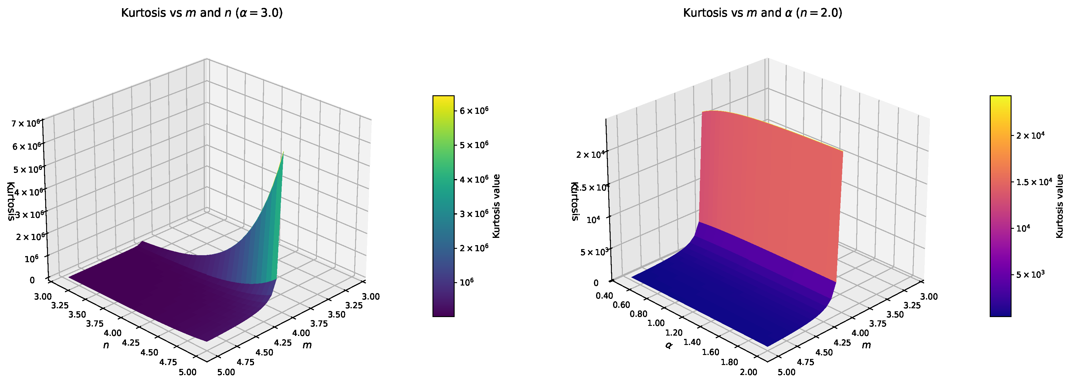
The kurtosis analysis of the BGD($\alpha$, m, n) distribution as portrayed in Figure 5 reveals pronounced heavy-tailed characteristics. For $\alpha =3.0$, extreme leptokurtosis (reaching ∼2.5 $\times {10}^6$) occurs at small m values ($4.0$–$4.4$), indicating frequent outlier events. With $n=2.0$, peak kurtosis (∼23) emerges at small $\alpha$ ($3.0$–$4.0$) and m combinations. Both parameters m and $\alpha$ strongly temper tail heaviness when increased. These properties make the distribution suitable for modeling extreme thunderstorm events with frequent severe occurrences.

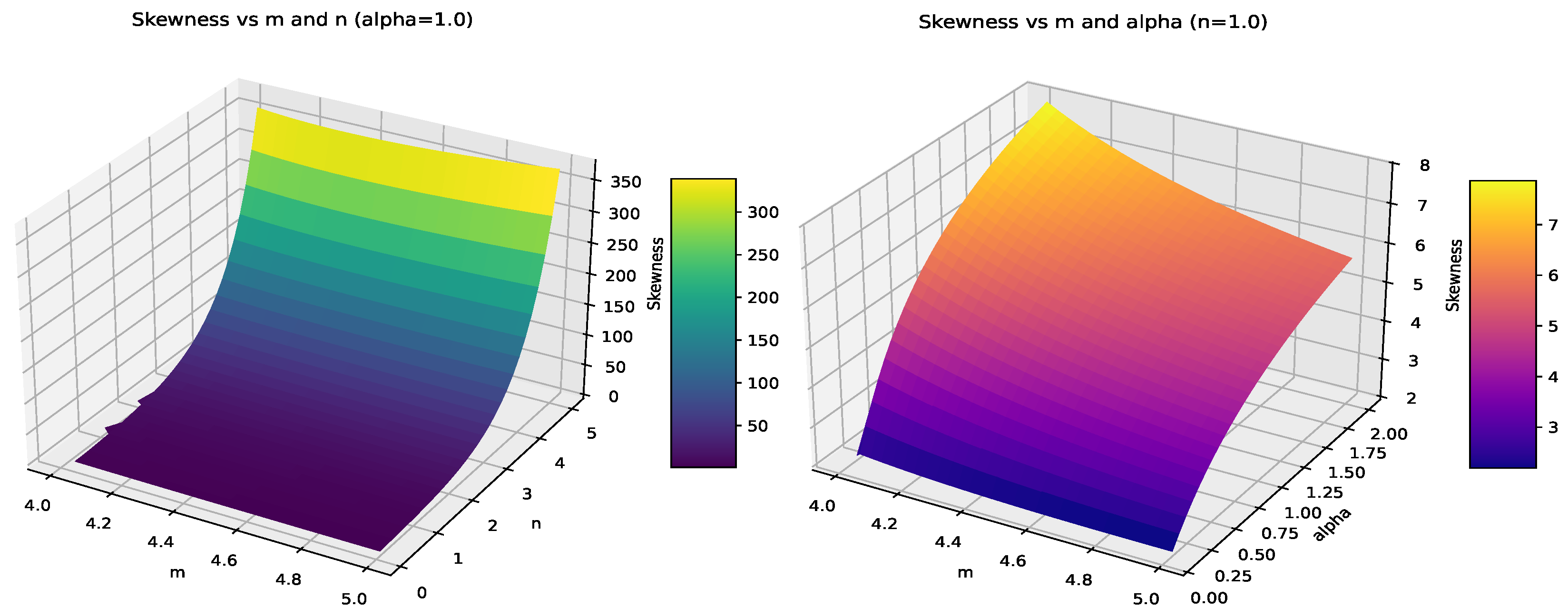
Figure 6 portrays skewness analysis of the GB($\alpha$, m, n) distribution which reveals strong right-skewness characteristics. For $\alpha =1.0$, extremely high positive skewness (reaching ∼300) occurs at small m ($4.0$–$4.4$) and moderate n (2–3) values, indicating pronounced right-tailed distributions. With $n=1.0$, skewness shows more moderate but still substantial positive values (∼7), peaking at small m ($4.0$–$4.4$) and intermediate $\alpha$ ($1.0$–$1.25$) combinations. In both cases, parameter m exerts strong control over asymmetry, with smaller m values generating more severely right-skewed distributions. These skewness patterns confirm the distribution’s capacity to model thunderstorm intensity data with frequent low-intensity events and occasional extreme values.

Remark 1.

If we substitute $e^t=t$ into Equation (4) then we get the probability generating function(PGF) of BGD($\alpha ,m,n$) defined as

$$G_X\left(t\right)={\displaystyle \frac{{\left(\alpha \right)}_{m}t}{{\left(\alpha \right)}_{m+n}}}{}_{2}F_1\left(\alpha ,n;\alpha +m+n;t\right).\alpha >0,m,n>0,$$

(5)

where ${\left(\alpha \right)}_k$ is the Pochhammer symbol (rising factorial) and ${}_{2}F_1$ is the Gauss hypergeometric function.

Factorial Moments

Let’s find the r-th factorial moment for the given PMF as defined in Equation (1). The r-th factorial moment is defined as: ${\mu }_{\left(r\right)}=E[X(X-1)(X-2)\cdots (X-r+1)].$ So, we need to compute: ${\mu }_{\left(r\right)}={\sum }_{x=1}^{\infty }[x(x-1)\cdots (x-r+1)]P(X=x).$ Let $k=x-1$, so $x=k+1$, and $k=0,1,2,\dots$. Then Equation (1) can be re written as

$$P(X=k+1)={\displaystyle \frac{{\left(\alpha \right)}_m}{{\left(\alpha \right)}_{m+n}}}·{\displaystyle \frac{{\left(\alpha \right)}_k{\left(n\right)}_k}{{(\alpha +m+n)}_{k}k!}}.$$

The factorial moment becomes

$${\mu }_{\left(r\right)}=\sum _{x=1}^{\infty }[x(x-1)\cdots (x-r+1)]P(X=x)=\sum _{k=0}^{\infty }[(k+1)k(k-1)\cdots (k-r+2)]P(X=k+1).$$

As

$$(k+1)k(k-1)\cdots (k-r+2)={\displaystyle \frac{(k+1)!}{(k-r+1)!}},$$

so

$${\mu }_{\left(r\right)}=\sum _{k=0}^{\infty }{\displaystyle \frac{(k+1)!}{(k-r+1)!}}·P(X=k+1).$$

Since the factorial in the denominator requires $k\ge r-1$, we can write

$${\mu }_{\left(r\right)}=\sum _{k=r-1}^{\infty }{\displaystyle \frac{(k+1)!}{(k-r+1)!}}·{\displaystyle \frac{{\left(\alpha \right)}_m}{{\left(\alpha \right)}_{m+n}}}·{\displaystyle \frac{{\left(\alpha \right)}_k{\left(n\right)}_k}{{(\alpha +m+n)}_{k}k!}}.$$

Let $j=k-(r-1)$, so $k=j+r-1$, $j=0,1,2,\dots$:

$${\mu }_{\left(r\right)}={\displaystyle \frac{{\left(\alpha \right)}_m}{{\left(\alpha \right)}_{m+n}}}\sum _{j=0}^{\infty }{\displaystyle \frac{(j+r)!}{j!}}·{\displaystyle \frac{{\left(\alpha \right)}_{j+r-1}{\left(n\right)}_{j+r-1}}{{(\alpha +m+n)}_{j+r-1}(j+r-1)!}}.$$

Observe that

$${\displaystyle \frac{(j+r)!}{j!}}=(j+r)(j+r-1)\cdots (j+1)={(r+1)}_j·r!,$$

and

$${\left(\alpha \right)}_{j+r-1}={\left(\alpha \right)}_{r-1}{(\alpha +r-1)}_j,$$

$${\left(n\right)}_{j+r-1}={\left(n\right)}_{r-1}{(n+r-1)}_j,$$

$${(\alpha +m+n)}_{j+r-1}={(\alpha +m+n)}_{r-1}{(\alpha +m+n+r-1)}_j,$$

$$(j+r-1)!=(r-1)!{\left(r\right)}_j.$$

Substituting all these

$${\mu }_{\left(r\right)}={\displaystyle \frac{{\left(\alpha \right)}_m}{{\left(\alpha \right)}_{m+n}}}·{\displaystyle \frac{r!{\left(\alpha \right)}_{r-1}{\left(n\right)}_{r-1}}{{(\alpha +m+n)}_{r-1}(r-1)!}}\times \sum _{j=0}^{\infty }{\displaystyle \frac{{(\alpha +r-1)}_j{(n+r-1)}_j}{{(\alpha +m+n+r-1)}_j}}·{\displaystyle \frac{1}{j!}}\times {\displaystyle \frac{{(r+1)}_j}{{\left(r\right)}_j}}.$$

As

$${\displaystyle \frac{{(r+1)}_j}{{\left(r\right)}_j}}={\displaystyle \frac{r+j}{r}},$$

so

$${\mu }_{\left(r\right)}={\displaystyle \frac{{\left(\alpha \right)}_m}{{\left(\alpha \right)}_{m+n}}}·{\displaystyle \frac{r{\left(\alpha \right)}_{r-1}{\left(n\right)}_{r-1}}{{(\alpha +m+n)}_{r-1}}}\times \sum _{j=0}^{\infty }{\displaystyle \frac{{(\alpha +r-1)}_j{(n+r-1)}_j}{{(\alpha +m+n+r-1)}_j}}·{\displaystyle \frac{1}{j!}}\times {\displaystyle \frac{r+j}{r}}.$$

(6)

Now, take sum only, i.e.

$$\mathrm{T}=\sum _{j=0}^{\infty }\left[{\displaystyle \frac{{(\alpha +r-1)}_j{(n+r-1)}_j}{{(\alpha +m+n+r-1)}_j}}{\displaystyle \frac{1}{j!}}\times 1\right]+\sum _{j=0}^{\infty }\left[{\displaystyle \frac{{(\alpha +r-1)}_j{(n+r-1)}_j}{{(\alpha +m+n+r-1)}_j}}{\displaystyle \frac{1}{j!}}\times {\displaystyle \frac{j}{r}}\right].$$

Now, using

$${}_{2}F_1(x,y;z;1)={\displaystyle \frac{\Gamma \left(z\right)\Gamma (z-x-y)}{\Gamma (z-x)\Gamma (z-y)}}(\Re (z-x-y)>0)$$

and applying it to both terms gives simplification

$$\mathrm{T}={\displaystyle \frac{\Gamma (\alpha +m+n+r-1)\Gamma (m-r)}{\Gamma (m+n)\Gamma (\alpha +m)}}·{\displaystyle \frac{r(m-r)+(\alpha +r-1)(n+r-1)}{r}},$$

and multiply by

$$\mathrm{F}={\displaystyle \frac{{\left(\alpha \right)}_m}{{\left(\alpha \right)}_{m+n}}}·{\displaystyle \frac{r{\left(\alpha \right)}_{r-1}{\left(n\right)}_{r-1}}{{(\alpha +m+n)}_{r-1}}}.$$

Now, incorporating $\mathrm{T}\times \mathrm{F}$ then substituting it into Equation (6), we get

$${\mu }_{\left(r\right)}={\displaystyle \frac{\Gamma (m-r)}{\Gamma (m+n)}}{\left(\alpha \right)}_{r-1}{\left(n\right)}_{r-1}\left(r(m-r)+(\alpha +r-1)(n+r-1)\right).$$

Now, a recurrsive relation between factorial moments can be established as

$${\displaystyle \frac{{\mu }_{(r+1)}}{{\mu }_{\left(r\right)}}}={\displaystyle \frac{(\alpha +r-1)(n+r-1)\left[(r+1)(m-r-1)+(\alpha +r)(n+r)\right]}{(m-r-1)\left[r(m-r)+(\alpha +r-1)(n+r-1)\right]}}.$$

4. Risk Measures for BGD($\mathit{\alpha },\mathit{m},\mathit{n}$)

Risk management is vital for financial institutions to evaluate and mitigate potential losses see [18]. While variance was once the main risk measure, its limitations led to advanced approaches like Value-at-Risk (VaR), Expected Shortfall (ES), Tail Variance (TV), Tail Variance Premium (TVP), and Mean Residual Life (MRL), which better capture extreme loss behavior. These modern measures improve the accuracy of tail risk assessment and capital allocation (see [19,20,21]).

4.1. Value at Risk (VaR)

VaR is one of the most widely used risk measures in finance for quantifying the potential loss in value of a portfolio or financial position over a specific time horizon at a given confidence level. For a random variable X representing losses (where higher values of X indicate greater losses), the VaR at level $\alpha \in (0,1)$ is defined as

$${\mathrm{VaR}}_{\alpha }\left(X\right)=inf\{x\in \mathbb{R}:P(X\le x)\ge \alpha \}.$$

In the case of a discrete distribution, the cumulative distribution function (CDF) $F_X\left(x\right)$ is a step function. Therefore, the $\rho$-quantile (VaR) corresponds to the smallest value $x_i$ such that

$$F_X\left(x_i\right)=\sum _{x_j\le x_i}{p}_j\ge \rho ,$$

where $p_j=P(X=x_j)$ denotes the probability mass at point $x_j$.

Interpretation 1.

The ${\mathit{VaR}}_{\alpha }$ represents the maximum loss that will not be exceeded with probability $\rho$. For example,${\mathit{VaR}}_{0.95}\left(X\right)$ gives the loss level that will be exceeded only 5% of the time. For BGD($\alpha ,m,n$) distribution,

$${\mathit{VaR}}_{\rho }\left(X\right)=min\left\{x\in \mathbb{N}:\sum _{k=1}^x{\displaystyle \frac{{\left(\alpha \right)}_m{\left(\alpha \right)}_{k-1}{\left(n\right)}_{k-1}}{{\left(\alpha \right)}_{m+n}{(\alpha +m+n)}_{k-1}(k-1)!}}\ge \rho \right\}.$$

(7)

Figure 7 illustrates the risk measure behavior of the BGD($\alpha ,m,n$) distribution with parameters $(\alpha =0.8,m=1,n=2)$, representing a very high risk scenario. The left panel shows that three risk measures (VaR, TVaR, TVP) all increase with confidence levels, with TVP being the most conservative. The right panel shows the MRL function increasing and plateauing over time, indicating a heavy-tailed distribution where substantial losses remain probable. Combined, these findings highlight the model’s suitability for analyzing extreme financial and insurance risks.

4.2. Expected Shortfall (ES) for Discrete Distribution

ES, also known as Conditional Value-at-Risk (CVaR), is a coherent risk measure that represents the expected loss given that the loss has exceeded the VaR at a specified confidence level $\rho$. For a discrete random variable X representing losses, the ES at level $\rho$ is defined as $E{S}_{\rho }\left(X\right)=\mathbb{E}[X\mid X\ge Va{R}_{\rho }\left(X\right)],$ where $Va{R}_{\rho }\left(X\right)$ denotes the $\rho$-quantile (or the smallest value x such that $P(X\le x)\ge \rho$). In the case of a discrete distribution, the loss variable X takes values $x_1,x_2,\dots ,x_n$ with corresponding probabilities $p_1,p_2,\dots ,p_n$ such that ${\sum }_{i=1}^n{p}_i=1$. To compute $E{S}_{\rho }\left(X\right)$,

• Sort the losses in ascending order: $x_{\left(1\right)}\le x_{\left(2\right)}\le \cdots \le x_{\left(n\right)}$.
• Compute the cumulative probabilities $F\left(x_{\left(i\right)}\right)={\sum }_{j=1}^i{p}_{\left(j\right)}$.
• Identify the Value-at-Risk $Va{R}_{\alpha }\left(X\right)=x_{\left(k\right)}$ such that $F\left(x_{(k-1)}\right)<\alpha \le F\left(x_{\left(k\right)}\right)$.
• Then, ES fall is calculated as the conditional expected loss beyond this threshold:

  $$E{S}_{\rho }\left(X\right)={\displaystyle \frac{{\sum }_{i=k}^n{x}_{\left(i\right)}{p}_{\left(i\right)}}{{\sum }_{i=k}^n{p}_{\left(i\right)}}}.$$

By using survival function, expression is written as

$${\mathrm{ES}}_{\rho }\left(X\right)={\mathrm{VaR}}_{\rho }\left(X\right)+{\displaystyle \frac{1}{1-\rho }}\sum _{x={\mathrm{VaR}}_{\rho }\left(X\right)+1}^{\infty }{S}_X\left(x\right).$$

Thus, ES provides the average of the worst $(1-\rho )$ proportion of losses, making it a more informative and risk-sensitive measure than VaR, particularly for distributions with heavy tails or extreme loss events. Now, for BGD($\alpha ,m,n$) distribution,

$${\mathrm{ES}}_{\rho }\left(X\right)={\displaystyle \frac{1}{1-\rho }}\sum _{x={\mathrm{VaR}}_{\rho }\left(X\right)}^{\infty }x·{\displaystyle \frac{{\left(\alpha \right)}_m{\left(\alpha \right)}_{x-1}{\left(n\right)}_{x-1}}{{\left(\alpha \right)}_{m+n}{(\alpha +m+n)}_{x-1}(x-1)!}}.$$

(8)

Figure 8 displays the risk measure profiles for the BGD($\alpha ,m,n$) distribution configured with parameters representing a low-risk scenario. The left plot likely illustrates three key risk metrics–VaR, TVaR, TV and Tail Variance Premium (TVP)–across various confidence levels. In a low-risk setting, we would expect these measures to be relatively low in magnitude and to exhibit a gentle, convergent trend, indicating a lower probability of severe extreme losses. The right plot presumably shows the MRL function, which would be characterized by a decreasing or stable trend, reflecting the expectation that residual risk diminishes over time in a benign environment. Collectively, these graphs demonstrate the flexibility of the BGD$(\alpha ,m,n)$ model in capturing the subdued tail behavior and reduced persistence of risk typical of low-risk applications.

4.3. Tail Variance

Let X be a discrete random variable representing losses, with PMF $p\left(x\right)$ and CDF $F\left(x\right)$. For a given threshold level $q_{\rho }$ (such as the $\rho$-quantile or VaR at confidence level $\rho$), the TV is defined as the conditional variance of losses exceeding this threshold. Mathematically, it is expressed as

$$T{V}_{\rho }\left(X\right)=\mathrm{Var}\left(X\mid X>q_{\rho }\right).$$

For a discrete distribution, this can be computed as

$$T{V}_{\rho }\left(X\right)=\sum _{x_i>q_{\rho }}{\left(x_i-\mathbb{E}[X\mid X>q_{\rho }]\right)}^2{\displaystyle \frac{p\left(x_i\right)}{1-F\left(q_{\rho }\right)}},$$

where $\mathbb{E}[X\mid X>q_{\rho }]$ is the conditional mean (Expected Shortfall or tail mean), given by

$$\mathbb{E}[X\mid X>q_{\rho }]={\displaystyle \frac{{\sum }_{x_i>q_{\rho }}{x}_{i}p\left(x_i\right)}{1-F\left(q_{\rho }\right)}}.$$

The TV quantifies the dispersion or variability of extreme losses beyond a specified quantile. While ES captures the average of tail losses, TV measures the uncertainty within this tail region. Hence, it provides a second-order assessment of tail risk, particularly useful for discrete loss distributions where extreme events occur with specific probabilities. For BGD($\alpha ,m,n$) it is expressed as

$${\mathrm{TV}}_{\rho }\left(X\right)={\displaystyle \frac{1}{1-\rho }}\sum _{x={\mathrm{VaR}}_{\rho }\left(X\right)}^{\infty }{\left(x-{\mathrm{ES}}_{\rho }\left(X\right)\right)}^2·{\displaystyle \frac{{\left(\alpha \right)}_m{\left(\alpha \right)}_{x-1}{\left(n\right)}_{x-1}}{{\left(\alpha \right)}_{m+n}{(\alpha +m+n)}_{x-1}(x-1)!}}.$$

(9)

Figure 9 presents the risk measure behavior of the BGD($\alpha ,m,n$) configured with parameters corresponding to a medium-risk scenario. The left panel, comparing VaR, TVaR, and TVP, likely shows these measures increasing at a moderate rate with the confidence level. The divergence between them is expected to be more pronounced than in a low-risk setting but less extreme than in a high-risk one, indicating a balanced exposure to potential tail losses. The right panel, depicting the MRL function, probably shows a curve that initially demonstrates stability or a gentle increase before eventually beginning to decrease, characterizing a scenario with moderate persistence of risk over time. Overall, these graphs effectively capture the intermediate characteristics of a medium-risk environment, showcasing the BGD$(\alpha ,m,n)$ model’s versatility in modeling a spectrum of risk profiles between the extremes of low and high severity.

4.4. Tail Variance Premium (TVP)

Let X be a discrete random variable representing loss, and let $\rho \in (0,1)$ denote the risk level or confidence level. The Tail Variance Premium (TVP) is a risk measure designed to capture the variability of extreme losses that exceed the Value-at-Risk (VaR) at level $\rho$. It refines the Expected Shortfall (ES) by incorporating the dispersion of losses in the tail region.

Mathematically, for a discrete loss distribution, the Tail Variance Premium is defined as:

$$TV{P}_{\rho }\left(X\right)=E{S}_{\rho }\left(X\right)+\lambda Var(X\mid X>Va{R}_{\rho }\left(X\right)),$$

where

• $E{S}_{\rho }\left(X\right)$ is the Expected Shortfall at level $\rho$;
• $Va{R}_{\rho }\left(X\right)$ is the Value-at-Risk at level $\rho$;
• $Var(X\mid X>Va{R}_{\rho }\left(X\right))$ denotes the conditional variance of losses exceeding the VaR threshold.

The parameter $\lambda >0$ serves as a sensitivity factor that determines the weight assigned to tail variability. Thus, the TVP accounts not only for the expected magnitude of extreme losses (captured by $E{S}_{\rho }$) but also for their uncertainty and dispersion beyond the threshold, making it a more comprehensive and robust measure of tail risk for discrete loss distributions. For BGD($\alpha ,m,n$) it is written as

$${\mathrm{TVP}}_{\rho }\left(X\right)={\mathrm{ES}}_{\rho }\left(X\right)+\lambda ·\sqrt{{\displaystyle \frac{1}{1-\rho }}\sum _{x={\mathrm{VaR}}_{\rho }\left(X\right)}^{\infty }{\left(x-{\mathrm{ES}}_{\rho }\left(X\right)\right)}^2·{\displaystyle \frac{{\left(\alpha \right)}_m{\left(\alpha \right)}_{x-1}{\left(n\right)}_{x-1}}{{\left(\alpha \right)}_{m+n}{(\alpha +m+n)}_{x-1}(x-1)!}}}.$$

(10)

Figure 10 demonstrates the flexibility of the BGD($\alpha ,m,n$) distribution by presenting risk measure graphs for a scenario of varied risk. Unlike previous figures with fixed parameters, this analysis likely explores the sensitivity of the risk measures to changes in one or more of the parameters $(\alpha ,m,n)$. The left panel, showing VaR, TVaR, and TVP, probably contains multiple curves that illustrate how the tail behavior and risk severity evolve across different parameter sets. This allows for a direct comparison of how slight modifications in the model’s shape can shift the risk profile from low to high. Similarly, the right panel’s MRL are expected to exhibit a family of curves, showcasing a range of aging properties from decreasing to increasing trends. This comprehensive view underscores the capacity of the BGD$(\alpha ,m,n)$ model to adapt and represent a wide spectrum of risk dynamics, making it a powerful tool for scenario analysis and stress-testing in financial and insurance modeling.

4.5. Mean Residual Life (MRL) Function

The MRL function is an important concept in reliability engineering and survival analysis. For a nonnegative random variable X (e.g., lifetime), the MRL function at time t is defined as

$$m\left(t\right)=\mathbb{E}[X-t\mid X>t]={\displaystyle \frac{{\sum }_t^{\infty }(x-t)P(X=x)}{S\left(t\right)}},$$

where $f\left(x\right)$ is the PDF (PMF for discrete cases) and $S\left(t\right)=P(X>t)$ is the survival function. As X∼ BGD($\alpha ,m,n$) and its PMF is defined in Equation (1). Let $k=x-1$, so $x=k+1$ and $k=0,1,2,\dots$. Then,

$$P(X=k+1)=C·{\left(\alpha \right)}_k{\left(n\right)}_k{(\alpha +m+n)}_k/k!,$$

(11)

where $C={\displaystyle \frac{{\left(\alpha \right)}_{m+n}}{{\left(\alpha \right)}_m}}$. As MRL Function at integer t $m\left(t\right)=E[X-t\mid X>t]={\sum }_{k=t}^{\infty }(k-t+1)P(X=k+1)$. On substituting $P(X=k+1)$ in Equation (11) we get $m\left(t\right)={\sum }_{k=t}^{\infty }(k-t+1)·C·{\left(\alpha \right)}_k{\left(n\right)}_k{(\alpha +m+n)}_k/k!$. Let $j=k-t$, so $k=j+t$, then

$$m\left(t\right)=\sum _{j=0}^{\infty }(j+1)·C·{(\alpha +t)}_j{(n+t)}_j{(\alpha +m+n+t)}_j/j!.$$

By using the identity ${\left(\alpha \right)}_j+t={\left(\alpha \right)}_t{(\alpha +t)}_j,(j+t)!=t!{(t+1)}_j$, we get

$$m\left(t\right)={\displaystyle \frac{{\left(\alpha \right)}_t{\left(n\right)}_t{(\alpha +m+n)}_t}{t!}}\sum _{j=0}^{\infty }{\displaystyle \frac{{(\alpha +t)}_j{(n+t)}_j{(\alpha +m+n+t)}_j}{{(t+1)}_{j}j!}},$$

which is a generalized hypergeometric series function:

$$\sum _{j=0}^{\infty }{\displaystyle \frac{{(\alpha +t)}_j{(n+t)}_j{(\alpha +m+n+t)}_j}{{(t+1)}_{j}j!}}={}_{3}F_2\left(\alpha +t,n+t,1;\alpha +m+n+t,t+1;1\right).$$

Similarly, the denominator series $D\left(t\right)={\sum }_{k=t}^{\infty }{\displaystyle \frac{{\left(\alpha \right)}_k{\left(n\right)}_k{(\alpha +m+n)}_k}{k!}}$ can be expressed as $D\left(t\right)={}_{2}F_1(\alpha ,n;\alpha +m+n;1)-{\sum }_{k=0}^{t-1}{\displaystyle \frac{{\left(\alpha \right)}_k{\left(n\right)}_k{(\alpha +m+n)}_k}{k!}}.$ Using the transformation ${\left(\alpha \right)}_j+t={\left(\alpha \right)}_t{(\alpha +t)}_j$ and similar identities, the numerator becomes $N\left(t\right)={\displaystyle \frac{{\left(\alpha \right)}_t{\left(n\right)}_t{(\alpha +m+n)}_t}{t!}}·{}_{4}F_3\left(2,\alpha +t,n+t,1;\alpha +m+n+t,\right.\left.t+1,1;1\right)$. Thus, the MRL of BG$(\alpha ,m,n)$

$$m\left(t\right)={\displaystyle \frac{N\left(t\right)}{D\left(t\right)}}={\displaystyle \frac{{}_{4}F_3\left(2,\alpha +t,n+t,1;\alpha +m+n+t,t+1,1;1\right)}{{}_{3}F_2\left(\alpha +t,n+t,1;\alpha +m+n+t,t+1;1\right)}}.$$

The graphs, as portrayed in Figure 11, potray that the MRL increases with $\alpha$ for different fixed values of m and n. The relationship appears linear, with the parameters m and n affecting the rate of increase, indicating how these parameters influence the residual life in the model.

Table 1. Risk Level and Parameters Sets.

S.#.	Label	$\mathit{\alpha }$	m	n	Mean	Std_Dev
1	Low Risk 1	2.0000	2	3	5.8197	6.8097
2	Low Risk 2	2.5000	3	4	5.6980	5.9367
3	Low Risk 3	3.0000	3	5	7.7980	7.4120
4	Medium Risk 1	1.5000	2	3	4.7373	5.9277
5	Medium Risk 2	2.0000	3	3	3.8957	4.3634
6	Medium Risk 3	2.5000	2	4	8.3684	8.5407
7	High Risk 1	1.0000	2	2	2.7818	3.8302
8	High Risk 2	1.5000	2	2	3.6018	4.7676
9	High Risk 3	2.0000	2	2	4.3793	5.5501
10	Very High Risk 1	0.8000	1	2	4.6373	7.0119
11	Very High Risk 2	1.0000	1	2	5.3191	7.5993
12	Very High Risk 3	1.2000	1	2	5.9460	8.0895
13	Conservative 1	3.0000	4	5	5.8762	5.5237
14	Conservative 2	3.5000	4	6	7.7087	6.7788
15	Conservative 3	4.0000	5	6	6.9046	5.8046
16	Balanced 1	2.0000	4	4	3.6407	3.6828
17	Balanced 2	2.5000	4	5	5.0867	4.9417
18	Balanced 3	3.0000	5	5	4.7261	4.2528
19	Varied 1	1.8000	3	3	3.6152	4.0939
20	Varied 2	2.2000	3	4	5.1659	5.5244
21	Varied 3	2.8000	4	4	4.6753	4.5630
22	Varied 4	3.2000	4	5	6.1884	5.7436
23	Varied 5	3.6000	5	5	5.4598	4.7929
24	Varied 6	4.0000	5	6	6.9046	5.8046
25	Varied 7	1.2000	2	3	4.0519	5.3027
26	Varied 8	1.6000	2	4	6.0581	7.0642
27	Varied 9	2.4000	3	5	6.5486	6.6114
28	Varied 10	2.6000	3	6	8.0170	7.6072

summarizes the different risk levels and their associated parameter sets defined by parameters $\alpha$, m, and n. The labels range from low risk to very high risk, including balanced, conservative, and varied categories. The parameters $\alpha$, m, and n govern the shape and scale of the corresponding probability distributions used in risk modeling. As the risk level increases from low to very high, the mean generally increases, indicating higher expected returns (or losses), while the standard deviation also increases, reflecting greater uncertainty and volatility. The varied and balanced sets represent mixed risk environments, providing diversity for comparative performance assessment under different distributional assumptions. Overall, this table provides a structured parameterization for simulation or empirical analysis of risk measures such as VaR, ES, TV, and TVP.

Table 2. Summary statistics for VaR, ES, TV, TVP, and MRL.

VaR_95	ES_95	TV_95	TVP_95	MRL
20.0000	28.9740	63.4069	36.9369	6.0427
17.0000	24.6329	58.9594	32.3114	5.5836
23.0000	31.0867	50.9053	38.2215	7.4225
16.0000	24.7108	71.0834	33.1419	5.1848
12.0000	18.2372	52.8021	25.5038	4.0563
27.0000	35.3686	43.3501	41.9527	8.2067
9.0000	15.5079	63.1852	23.4569	3.5714
12.0000	19.7267	70.8393	28.1433	4.2132
15.0000	23.4850	71.5497	31.9438	4.8405
19.0000	29.5131	75.3514	38.1936	6.1596
22.0000	32.1479	64.0716	40.1523	6.6109
24.0000	33.7943	56.5513	41.3144	7.0431
16.0000	22.5836	49.8922	29.6470	5.5502
21.0000	28.3674	49.5243	35.4047	7.1863
18.0000	24.3208	44.4397	30.9871	6.3493
10.0000	14.6263	34.8469	20.5294	3.6569
14.0000	20.0633	46.9789	26.9175	4.8813
13.0000	17.9535	35.1811	23.8849	4.4313
11.0000	16.8792	50.0640	23.9548	3.8307
16.0000	23.4015	58.6519	31.0599	5.1413
13.0000	18.6811	44.0014	25.3145	4.5030
17.0000	23.7772	50.4624	30.8809	5.8201
14.0000	19.3774	38.7863	25.6053	5.0581
18.0000	24.3208	44.4397	30.9871	6.3493
14.0000	22.3298	72.3710	30.8369	4.6615
20.0000	29.0529	63.8274	37.0421	6.3125
20.0000	27.9955	56.3247	35.5005	6.3453
24.0000	32.0679	48.7140	39.0474	7.6513

reports the VaR, ES, TV, TVP, and MRL at the 95% confidence level for various scenarios. VaR_0.95 represents the threshold value below which 95% of losses fall, i.e., the worst expected loss over a specified time horizon. ES_0.95 averages the losses beyond VaR, providing a more coherent and conservative measure of tail risk. TV_0.95 quantifies the variability of losses beyond the VaR threshold, while TVP_0.95 further adjusts TV by adding a premium term to account for the dispersion in the tail. MRL indicates the expected loss exceeding the VaR level, reflecting how the mean tail behavior evolves with extreme outcomes. From the table, it is evident that as VaR and ES increase, the TV and TVP also tend to rise, demonstrating consistency in tail sensitivity across risk levels. The TVP values are consistently higher than TV, confirming that the premium adjustment amplifies the representation of extreme tail risks. MRL values vary moderately, showing the expected magnitude of exceedance beyond VaR. In conclusion, the combined analysis of VaR, ES, TV, TVP, and MRL provides a comprehensive evaluation of both the magnitude and variability of extreme financial risks, highlighting the usefulness of tail-based risk measures in discrete loss distributions.

5. Characterization

Characterization is a cornerstone of probability theory that enables identification, simplification, and deeper understanding of distributions. The following theorem provides a characterization via the Fourier transform, which is both theoretically elegant and practically useful.

Theorem 2.

Let X be a random variable with characteristic function:

$${\varphi }_X\left(t\right)=e^{it}{\displaystyle \frac{{\left(\alpha \right)}_m}{{\left(\alpha \right)}_{m+n}}}{}_{2}F_1\left(\alpha ,n;\alpha +m+n;e^{it}\right),$$

(12)

where $\alpha >0$, $m,n\in \mathbb{N}$, and ${}_{2}F_1$ is the Gaussian hypergeometric function. Then X uniquely follows the distribution with PMF as defined in Equation (1).

Proof. 

Necessity:

As the Fourier transform (or characteristic function) of a discrete random variable X is given by ${\varphi }_X\left(t\right)=\mathbb{E}\left[e^{itX}\right]={\sum }_{x=1}^{\infty }{e}^{itx}P(X=x)$. If X $\sim \mathrm{BGD}(\alpha ,m,n)$ then its discrete fourier transformation is expressed as

$${\varphi }_X\left(t\right)=\sum _{x=1}^{\infty }{e}^{itx}\left[{\displaystyle \frac{{\left(\alpha \right)}_m}{{\left(\alpha \right)}_{m+n}}}·{\displaystyle \frac{{\left(\alpha \right)}_{x-1}{\left(n\right)}_{x-1}}{{(\alpha +m+n)}_{x-1}(x-1)!}}\right].$$

Let $k=x-1$, so $x=k+1$. As x goes from 1 to ∞, k goes from 0 to ∞. Then:

$${\varphi }_X\left(t\right)=\sum _{k=0}^{\infty }{e}^{it(k+1)}\left[{\displaystyle \frac{{\left(\alpha \right)}_m}{{\left(\alpha \right)}_{m+n}}}·{\displaystyle \frac{{\left(\alpha \right)}_k{\left(n\right)}_k}{{(\alpha +m+n)}_{k}k!}}\right].$$

Take $e^{it}$ as common, then

$${\varphi }_X\left(t\right)=e^{it}{\displaystyle \frac{{\left(\alpha \right)}_m}{{\left(\alpha \right)}_{m+n}}}\sum _{k=0}^{\infty }\left[e^{itk}{\displaystyle \frac{{\left(\alpha \right)}_k{\left(n\right)}_k}{{(\alpha +m+n)}_{k}k!}}\right],$$

where the sum can be written as

$$\sum _{k=0}^{\infty }{\displaystyle \frac{{\left(\alpha \right)}_k{\left(n\right)}_k}{{(\alpha +m+n)}_{k}k!}}{\left(e^{it}\right)}^k={}_{2}F_1(\alpha ,n;\alpha +m+n;e^{it}).$$

Thus, we have

$${\varphi }_X\left(t\right)=e^{it}{\displaystyle \frac{{\left(\alpha \right)}_m}{{\left(\alpha \right)}_{m+n}}}·{}_{2}F_1(\alpha ,n;\alpha +m+n;e^{it}),$$

where ${}_{2}F_1$ is the Gaussian hypergeometric function.

Suffiency: Let the Equation (12) holds then the integer-valued X, the PMF is recovered from the characteristic function by

$$p_x=\mathbb{P}(X=x)={\displaystyle \frac{1}{2\pi }}{\int }_{-\pi }^{\pi }{\varphi }_X\left(t\right)e^{-itx}dt,x\in \mathbb{Z}.$$

Use the hypergeometric series (valid on the unit circle by analytic continuation and absolute convergence of the coefficients) as

$${\varphi }_X\left(t\right)={\displaystyle \frac{{\left(\alpha \right)}_m}{{\left(\alpha \right)}_{m+n}}}\sum _{k=0}^{\infty }{\displaystyle \frac{{\left(\alpha \right)}_k{\left(n\right)}_k}{{(\alpha +m+n)}_k}}{\displaystyle \frac{e^{it(1+k)}}{k!}}.$$

According to inverse discrete fourier transformation, we have

$$p_x={\displaystyle \frac{{\left(\alpha \right)}_m}{{\left(\alpha \right)}_{m+n}}}\sum _{k=0}^{\infty }{\displaystyle \frac{{\left(\alpha \right)}_k{\left(n\right)}_k}{{(\alpha +m+n)}_k}}{\displaystyle \frac{1}{k!}}·{\displaystyle \frac{1}{2\pi }}{\int }_{-\pi }^{\pi }{e}^{it(1+k-x)}dt.$$

by the use of Fourier orthaganality we have

$${\displaystyle \frac{1}{2\pi }}{\int }_{-\pi }^{\pi }{e}^{it(1+k-x)}dt=\left\{\begin{array}{cc}1,\hfill & x=1+k,\hfill \\ 0,\hfill & x\ne 1+k,\hfill \end{array}\right.$$

i.e., a Kronecker delta ${\delta }_{x,k+1}$, which picks out exactly one term in the sum: $k=x-1$ (requiring $x\ge 1$), so, for $x=1,2,3,·$ we have the Equation (1). By using the Cauchy coefficient formula we let $z=e^{it}$. Then

$$p_x={\displaystyle \frac{1}{2\pi i}}{\oint }_{\left|t\right|=1}\underset{=G_X\left(t\right)}{\underbrace{\left[{\displaystyle \frac{{\left(\alpha \right)}_m}{{\left(\alpha \right)}_{m+n}}}t{}_{2}F_1(\alpha ,n;\alpha +m+n;t)\right]}}{t}^{-x-1}dt,$$

which, by Cauchy’s formula, extracts the coefficient of $t^x$ in $G_X\left(t\right)$, giving the Equation (5). This completes the proof. □

6. Parameter Estimation

In probability and statistics, parameter estimation refers to the process of using sample data to estimate the parameters of a theoretical probability distribution. Parameter estimation is grounded in statistical theory aimed at deriving estimators with optimal properties. The common goals of estimation are (i) to determine the most likely values of unknown parameters, (ii) to describe the population behavior using the estimated model, and (iii) to perform prediction and inference based on the fitted model. We have estimated the parameters by maximum likelihood method.

6.1. Maximum Likelihood Estimation (MLE) via Grid Search

MLE is one of the most important and widely used methods for parameter estimation in statistics. Its primary goal is to find parameter values that maximize the likelihood of observing the given data, thereby making the observed sample most probable under the assumed model. Beyond its intuitive appeal, MLE possesses several crucial asymptotic properties—such as consistency (converging to the true parameter as the sample size grows) and efficiency (achieving the lowest possible variance among unbiased estimators under regular conditions). These properties make MLE a cornerstone of modern statistical inference. Formally, MLE estimates parameters by maximizing the likelihood function. For a sample $x_1,x_2,\dots ,x_N$, the likelihood is given by

$$L(\alpha ,m,n)=\prod _{i=1}^{N}P(x_i;\alpha ,m,n)=\prod _{i=1}^N{\displaystyle \frac{{\left(\alpha \right)}_m}{{\left(\alpha \right)}_{m+n}}}{\displaystyle \frac{{\left(\alpha \right)}_{x_i-1}{\left(n\right)}_{x_i-1}}{{(\alpha +m+n)}_{x_i-1}(x_i-1)!}}.$$

The log-likelihood is

$$\begin{array}{cc}\hfill \ell (\Theta )=& logL=N\left[log\Gamma (\alpha +m)-log\Gamma \left(\alpha \right)-log\Gamma \left(n\right)\right]+\sum _{i=1}^N\left[log\Gamma (\alpha +x_i-1)+log\Gamma (n+x_i-1)\right.\hfill \\ \hfill & \left.-log\Gamma (\alpha +m+n+x_i-1)-log\Gamma \left(x_i\right)\right].\hfill \end{array}$$

(13)

It can be composed as

$$\ell (\alpha ,m,n|\mathbf{x})=N·\left[\sum _{j=0}^{m-1}log(\alpha +j)-\sum _{j=0}^{m+n-1}log(\alpha +j)\right]+\sum _{i=1}^{N}g(x_i,\alpha ,m,n),$$

where for $x_i>1$ it can be rewritten as

$$g(x_i,\alpha ,m,n)=\sum _{j=0}^{x_i-2}log(\alpha +j)+\sum _{j=0}^{x_i-2}log(n+j)-\sum _{j=0}^{x_i-2}log(\alpha +m+n+j)-log((x_i-1)!).$$

As $\widehat{\alpha }>0,\widehat{m}\in {\mathbb{Z}}^{+}\left(\mathrm{positive}\mathrm{integer}\right),\widehat{n}\in {\mathbb{Z}}^{+}\left(\mathrm{positive}\mathrm{integer}\right)$, so for maximization of $m,n$ we shall use grid serach over reasonable ranges i.e., $min\{1,2,3,..., M_{max}$, $N\in 1,2,3,...,N_{max}\}$. For each pair $(m,n)$ optimize $\alpha$ using numerical methods (e.g., gradient-based optimization see [22]) with relaxed constraints. For fixed m and n, maximize

$$\ell \left(\alpha \right|m,n,\mathbf{x})=N·A(m,n,\alpha )+\sum _{i=1}^{N}B(x_i,m,n,\alpha ),$$

where $A(m,n,\alpha )={\sum }_{j=0}^{m-1}log(\alpha +j)-{\sum }_{j=0}^{m+n-1}log(\alpha +j)$ and

$$B(x_i,m,n,\alpha )=\left\{\begin{array}{cc}0\hfill & \mathrm{if}{x}_i=1\hfill \\ \sum _{j=0}^{x_i-2}log(\alpha +j)-\sum _{j=0}^{x_i-2}log(\alpha +m+n+j)+C(x_i,n)\hfill & \mathrm{if}{x}_i>1\hfill \end{array}\right.$$

with $C(x_i,n)={\sum }_{j=0}^{x_i-2}log(n+j)-log((x_i-1)!)$. For gradient calculations, we have

$${\displaystyle \frac{\partial \ell }{\partial \alpha }}=N·\left[\sum _{j=0}^{m-1}{\displaystyle \frac{1}{\alpha +j}}-\sum _{j=0}^{m+n-1}{\displaystyle \frac{1}{\alpha +j}}\right]+\sum _{i:x_i>1}\left[\sum _{j=0}^{x_i-2}{\displaystyle \frac{1}{\alpha +j}}-\sum _{j=0}^{x_i-2}{\displaystyle \frac{1}{\alpha +m+n+j}}\right],$$

while its second derivative can be expressed as

$${\displaystyle \frac{{\partial }^2\ell }{\partial {\alpha }^2}}=-N·\left[\sum _{j=0}^{m-1}{\displaystyle \frac{1}{{(\alpha +j)}^2}}-\sum _{j=0}^{m+n-1}{\displaystyle \frac{1}{{(\alpha +j)}^2}}\right]-\sum _{i:x_i>1}\left[\sum _{j=0}^{x_i-2}{\displaystyle \frac{1}{{(\alpha +j)}^2}}-\sum _{j=0}^{x_i-2}{\displaystyle \frac{1}{{(\alpha +m+n+j)}^2}}\right].$$

6.2. Algorithm Implemention

In order to estimate MLEs, we used the attached algorithm as Step 1: (i) Set $M_{max},N_{max}$. (ii) Initialize $\mathrm{best}\_\mathrm{ll}=-\infty$. (iii) Initialize $\mathrm{best}\_\mathrm{params}=\mathrm{None}$. Step 2: For $m=1$ to $M_{max}$ and for $n=1$ to $N_{max}$, we used the grid iteration as follows: (i) Optimize $\alpha$: ${max}_{\alpha >0}\ell \left(\alpha \right|m,n,\mathbf{x})$; (ii) calculate likelihood: $\ell ({\alpha }^{*},m,n|\mathbf{x})$; and (iii) update the best parameters if improved. Step 3: For $\alpha$ optimization (fixed $m,n$), we used Newton–Raphson as

$${\alpha }_{k+1}={\alpha }_k-{\left[{\displaystyle \frac{{\partial }^2\ell }{\partial {\alpha }^2}}\right]}^{-1}·{\displaystyle \frac{\partial \ell }{\partial \alpha }}.$$

Finally, we obtain MLEs as $\widehat{m},\widehat{n},\widehat{\alpha }=arg{max}_{m,n,\alpha }\ell (\alpha ,m,n|\mathbf{x})$. This procedure usually have the following properties (i) The log-likelihood is differentiable w.r.t. $\alpha$. (ii) The parameters are identifiable for $m,n\ge 1$. (iii) The Fisher information matrix exists and is positive definite. Moreover, $\widehat{\Theta }$ is asymptotically trivariate Normal distribution as

$$\sqrt{N}\left(\left[\begin{array}{c}\widehat{\alpha }\\ \widehat{m}\\ \widehat{n}\end{array}\right]-\left[\begin{array}{c}{\alpha }_0\\ m_0\\ n_0\end{array}\right]\right)\stackrel{d}{\to }N(0,I^{-1}\left({\theta }_0\right)),$$

with information expressed as $\mathbb{I}(\Theta )=-\mathbb{E}\left[{\displaystyle \frac{{\partial }^2\ell }{\partial \Theta \partial {\Theta }^T}}\right]$.

7. Application

Modeling the number of thunderstorms at the Kennedy Space Center (KSC) in Florida, USA, is a classic application of count data models see [23]. The unique meteorological and geographical context makes it a compelling case study. The Kennedy Space Center is located on the Atlantic coast of Florida, a region known as the “Lightning Alley of the United States.” This presents a high-frequency, volatile environment for thunderstorms, driven by

• Sea Breezes: The convergence of sea breezes from both the Atlantic Ocean and the Gulf of Mexico provides a daily trigger for deep convection during much of the year.
• High Moisture Content: Proximity to warm ocean waters ensures a plentiful supply of atmospheric moisture, a key ingredient for thunderstorm development.
• Synoptic Weather Patterns: Seasonal patterns, such as the summer wet season and the passage of winter cold fronts, modulate the frequency and intensity of thunderstorm activity.

7.1. The Meteorological and Geographical Context

The empirical analysis utilizes a classic and high-resolution dataset of thunderstorm activity from the Kennedy Space Center (KSC), originally published by [24]. This dataset was compiled from WBAN-10 weather reports over an 31-year period (January 1957–December 1967). A critical characteristic of this data is that it is inherently zero-truncated; it only records days on which at least one thunderstorm event (THE) occurred. This is because the primary operational concern is understanding the intensity and internal structure of active storm days, rather than predicting the simple occurrence of any storm. Consequently, our model and the subsequent analysis are applied to this conditional dataset, focusing on the number of individual thunderstorms (THs) per event, where the count X satisfies $X\ge 1$. The sample sizes for the analyzed winter months are as follows: January ($n=8$), February ($n=23$), November ($n=15$), December ($n=13$), and the aggregate winter season ($n=44$). Following the foundational work of [24], who modeled this data using a Compound Negative Binomial-Positive Binomial distribution, we apply the more flexible BGD model to the same thunderstorm count data from Cape Kennedy (now KSC). This allows for a direct comparison of modern distributional techniques against a classical benchmark in meteorological statistics.

7.2. Motivation

The motivation for precise modeling at KSC is exceptionally high-stakes:

• Launch Safety: A thunderstorm within a certain radius is a launch commit criteria violation. Accurate probabilistic forecasts of thunderstorm likelihood are critical for scheduling and scrubbing launch attempts, which involve immense costs.
• Asset Protection: Spacecraft, rockets, and ground infrastructure are highly sensitive to lightning strikes. Models help assess lightning risk and inform decisions about when to keep hardware on the pad or roll it back to the protection of the Vehicle Assembly Building.
• Ground Operations: Outdoor work by personnel is halted during lightning warnings. A good model helps in planning work schedules to minimize downtime and ensure worker safety.
• Climatological Risk Assessment: Long-term models (e.g., using monthly/seasonal counts over decades) are used to understand the climatology of thunderstorm activity, which informs the design of structures and electrical systems to withstand lightning strikes.

7.3. Zero-Truncation Modeling

A zero-truncated distribution is desirable because decision-making at the Kennedy Space Center apprehensions only current thunderstorm events, making zero counts unconnected. Operational risks naturally exclude zero from the data. Furthermore, the following arguments support the use of zero-truncated modeling:

• The Launch Commit Criterion (LCC) states that having a thunderstorm within a certain distance automatically violates launch safety rules see [25]. Therefore, once a thunderstorm event (THE) begins, the focus shifts from predicting whether a storm will occur to estimating how many thunderstorms will form and how long the event will last. Since the event has already started, the count of storms begins at one, and the model provides the required real-time probabilities $P(X=x\mid X\ge 1)$ for decision-making.
• When a thunderstorm event happens, the financial and safety risks upsurge rapidly as the number of thunderstorms increases. One storm might source only a minor delay, but several storms in succession can force a complete launch cancellation, including the expensive technique of challenging the rocket’s fuel. Fortification procedures for spacecraft and ground facilities also depend on how intense and long the event becomes. By modeling the number of thunderstorms given that an event has already started, the BGD distribution offers the key probabilities needed to assess the chances of these high-risk, multiple-storm situations.
• The Carter’s ([24] data, taken from WBAN-10 forms, is naturally zero-truncated because a form is only started after thunder is first heard—meaning at least one thunderstorm has already occurred. Therefore, the dataset represents a conditional sample that begins only once a weather threat is active, matching the real-world conditions faced by forecasters and risk managers during an ongoing thunderstorm event.

7.4. Thunderstorm Activities in Winter Season

The analysis of thunderstorm events in November, December, January, February and the winter season at a location like Kennedy Space Center (KSC) is statistically and operationally significant, primarily because of its rarity and unique causation. During winter at Cape Kennedy, thunderstorm activity is infrequent and characterized by simplicity. On days with thunderstorms (THEs), the average number is about 1.19 per day, with most THEs containing only a single thunderstorm (TH). Approximately 20% of winter THEs have multiple THs, with a maximum of three within a single event. Overall, winter thunderstorms are rare, generally simple, and exhibit limited internal complexity. Approximately 80.6% of winter THEs contain only one thunderstorm (TH), about 12.9% contain two THs, and 6.5% contain three THs. No THEs with four or five THs are observed during the winter months.

7.5. Meteorological Significance

Winter THEs are typically driven by frontal systems rather than thermal convection, and are associated with synoptic-scale forcing rather than local sea breezes. They exhibit lower instability but stronger lift mechanisms. Due to their synoptic-scale organization, winter THEs may be more predictable. Although less frequent, winter thunderstorms can still produce severe weather such as strong winds, isolated tornadoes, and heavy rainfall.

7.6. Practical Applications for Space Operations

• Winter-Specific Planning: Due to the characteristics of winter THEs, space operations can benefit from the following: launch windows are fewer overall, but when they occur, they are typically single events; schedules can be optimized by planning around frontal passages more reliably; and risk assessment can be conducted with a lower probability of multiple THEs disrupting extended operations.
• Model Utility: The compound model remains valid for winter THEs, but with different parameter values. This allows for simpler approximations to be used for quick winter assessments. However, separate seasonal models are recommended for accurate planning.

7.7. Model Selection and Evaluation Statistics

In statistical modeling, especially with non-nested models (models that cannot be derived from one another by imposing parameter constraints), selecting the best model requires a suite of tests and criteria. These metrics balance model fit with complexity to prevent overfitting and identify the most parsimonious and plausible model.

• Akaike Information Criterion (AIC) is an estimator of prediction error. It measures the relative quality of a statistical model for a given dataset. It deals with the trade-off between the goodness-of-fit of the model and the complexity of the model (number of parameters). $\mathrm{AIC}=2k-2ln\left(\widehat{L}\right)$ where k is the number of estimated parameters and $\widehat{L}$ is the maximum value of the likelihood function. A lower AIC value indicates a better model. When comparing models, the one with the lowest AIC is preferred. A difference of more than 2 ($\Delta \mathrm{AIC}>2$) is generally considered substantial. Ref. [26] is the seminal text. Its philosophy is foundational in modern model selection.
• Bayesian Information Criterion (BIC) is similar to AIC but with a stronger penalty for model complexity, especially as sample size increases. It is derived from a Bayesian perspective. $\mathrm{BIC}=kln\left(n\right)-2ln\left(\widehat{L}\right)$ where n is the sample size. Like AIC, a lower BIC is better. BIC tends to favor simpler models more than AIC does, particularly with larger datasets. Ref. [27] provide an excellent overview of its use and interpretation in a practical context.
• Chi-Square (${\chi }^2$) Goodness-of-Fit Test is a classic test to assess how well a model’s predicted frequencies match the observed frequencies. It is a measure of absolute fit. ${\chi }^2={\sum }_i{\displaystyle \frac{{(O_i-E_i)}^2}{E_i}}$ where $O_i$ is the observed frequency and $E_i$ is the expected (predicted) frequency from the model. A lower ${\chi }^2$ value indicates a better fit see [28]. The associated p-value determines if the discrepancy is statistically significant. A p-value $>0.05$ (or a higher alpha level) suggests that there is no significant difference between the observed and predicted data, meaning the model fits well.
• p-Value quantifies the probability of obtaining test results at least as extreme as the observed results, assuming that the null hypothesis is true see [29]. For Goodness-of-Fit (Chi-square): The null hypothesis is “the model fits the data well.” A small p-value (e.g., <0.05) provides evidence against the null hypothesis, leading to the model’s rejection. A large p-value indicates that the observed discrepancy is consistent with random chance, so the model is not rejected. For Vuong Test: The interpretation is nuanced (see below).
• Vuong Statistic is a likelihood-ratio-based test for comparing non-nested models (i.e., models that are not special cases of each other). It can determine which of two models is closer to the true data-generating process and whether the difference is statistically significant. A large positive test statistic (e.g., >+1.96) significantly favors Model 1. A large negative test statistic (e.g., <−1.96) significantly favors Model 2. A test statistic close to zero (between $-1.96$ and $+1.96$) means the models are statistically indistinguishable. The accompanying p-value for this test indicates whether the statistic is significant. A p-value $<0.05$ typically leads to a decision for one model, while a p-value $>0.05$ leads to “No Decision”see [30].

In summary, these statistics form a powerful toolkit: AIC/BIC for initial ranking, the Chi-square test for checking absolute fit, and the Vuong test for a rigorous statistical comparison between the top non-nested candidates, with p-values guiding the final statistical decision in each test.

7.8. Data Analysis and Interpretation

Here we shall present a breif analysis of Thunderstorm event data sets ranging from January, February, November, December, and the winter season. Analysis covers Information Criterion, Goodness of Fit measures, Vuong statistics and line plots of the above mentioned data sets which are taken from [24].

Interpretation Based on Information Criterion: Based on the data provided in the paper by [24], we can perform a detailed analysis.

Table A1. Model fit statistics for different distributions for January Data.

Distribution	Parameters	$-\mathit{\ell }$	AIC	BIC
BGD	$\alpha =0.133$, $m=1$, $n=1$	−3.773886	13.547773	13.786097
ZTGP	$\theta =1.125$, $\lambda =-0.500$	−4.887516	13.775033	13.933916
SBNB	$r=2.000$, $p=0.500$	−15.942385	35.884770	36.043653
ZTGNB	$r=2.000$, $\beta =0.500$	−16.347850	36.695701	36.854584

,

Table A4. Model fit statistics for different distributions for February Data.

Distribution	Parameters	$-\mathit{\ell }$	AIC	BIC
BGD	$\alpha =0.248$, $m=1$, $n=1$	−17.073807	40.147613	43.554096
ZTGP	$\theta =1.261$, $\lambda =-0.500$	−17.477651	38.955302	41.226290
SBNB	$r=2.000$, $p=0.500$	−44.243637	92.487273	94.758261
ZTGNB	$r=2.000$, $\beta =0.500$	−46.388745	96.777490	99.048479

,

Table A7. Model fit statistics for different distributions for November Data.

Distribution	Parameters	$-\mathit{\ell }$	AIC	BIC
BGD	$\alpha =0.142,m=1,n=1$	7.419052	20.838103	22.962254
ZTGP	$\theta =1.133,\lambda =-0.500$	9.207873	22.415746	23.831846
SBNB	$r=2.000,p=0.500$	29.805329	63.610658	65.026758
ZTGNB	$r=2.000,\beta =0.500$	30.616259	65.232518	66.648618

,

Table A10. Model fit statistics for different distributions for December Data.

Distribution	Parameters	$-\mathit{\ell }$	AIC	BIC
BGD	$\alpha =0.080$, $m=1$, $n=1$	4.258589	14.5171	16.2120
ZTGP	$\theta =1.077$, $\lambda =-0.500$	7.6722	19.344579	20.474478
SBNB	$r=2.000$, $p=0.500$	26.3395	56.6791	57.8090
ZTGNB	$r=2.000$, $\beta =0.500$	−26.7450	57.4901	58.6200

and

Table A14. Model fit statistics for different distributions for winter Data.

Distribution	Parameters	$-\mathit{\ell }$	AIC	BIC
BGD	$\alpha =0.174$, $m=1$, $n=1$	25.729781	57.459563	62.812132
ZTGP	$\theta =1.182$, $\lambda =-0.500$	30.932044	65.864087	69.432467
SNBD	$r=2.000$, $p=0.500$	86.525615	177.051229	180.619608
ZTGNB	$r=2.000$, $\beta =0.500$	89.481653	182.963307	186.531686

in Appendix A portrayed a combined analysis of the model fit statistics across all five datasets reveals a consistent and clear hierarchy in the performance of the four candidate distributions. The BGD emerges as the unequivocally superior model. In every single dataset, the BGD consistently demonstrates the lowest Akaike Information Criterion (AIC) and Bayesian Information Criterion (BIC) values, which are key metrics for comparing models where lower values indicate a better balance of fit and complexity. This indicates that the BGD provides the most parsimonious and effective representation of the underlying data structure. The ZTGP model consistently ranks as the second-best option, with its AIC and BIC values being higher than those of the BGD but significantly lower than the remaining two models.

In stark contrast, the SBNB and ZTGNB models perform poorly across the board. Their AIC and BIC values are dramatically higher, often by a factor of two or three, clearly identifying them as the worst-fitting models for these datasets. This poor performance is likely due to their inflexibility, as their parameters (r, p, $\beta$) remain fixed across all analyses, whereas the key parameters of the BGD and ZTGP adapt to each dataset.

Therefore, the conclusive finding is that the BGD is the most appropriate and recommended model for this family of data.

Interpretation Based on Goodness of Fit Measures: The goodness-of-fit analysis as indicated in

Table A2. ${\chi }^2$ of X thunderstorms in January at Cape Kennedy.

x	Frequency	BGD	SBNB	ZTGP	ZTGNB
1	7	7.0622	9.0	4.3264	1.000
2	1	0.4396	18.0	4.4582	1.3333
3	0	0.1589	20.25	0.0918	1.3333
${\chi }^2$	8	0.7150	36.75	4.336	36.083
p-value		0.398	0.0000	0.037	0.0000

,

Table A5. ${\chi }^2$ of X thunderstorms in February at Cape Kennedy.

x	Frequency	BGD	SBNB	ZTGP	ZTGNB
1	18	18.43	2.88	11.47	2.88
2	4	2.03	5.75	14.39	3.83
3	1	0.78	6.47	1.06	3.83
4	0	0.41	5.75	0.00	3.41
${\chi }^2$		1.7071	25.3642	11.2219	36.9516
p-value		0.1913	0.0000	0.0000	0.0000

,

Table A8. ${\chi }^2$ of X thunderstorms in November at Cape Kennedy.

x	Frequency	BGD	SBNB	ZTGP	ZTGNB
1	13	13.132746	1.875000	8.072203	1.875000
2	2	0.871659	3.750000	8.428915	2.500000
${\chi }^2$		1.4619	15.6250	7.9117	25.8035
p-value		0.2266	0.0000	0.0000	0.0000

,

Table A11. ${\chi }^2$ of X thunderstorms in December at Cape Kennedy.

x	Frequency	BGD	SBNB	ZTGP	ZTGNB
1	12	12.038405	1.625000	7.232776	1.625000
2	1	0.462333	3.250000	6.879711	2.166667
3	0	0.162105	3.656250	0.058168	2.166667
4	0	0.082639	3.250000	−0.409123	1.925926
${\chi }^2$		0.6254	13.5416	8.1672	22.3630
p-value		0.4290	0.0000	0.0000	0.0000

and

Table A13. ${\chi }^2$ of X thunderstorms in Winter at Cape Kennedy.

x	Frequency	BGD	SNBD	ZTGP	ZTGNB
1	37	37.47	5.50	23.01	5.50
2	6	3.00	11.00	25.86	7.33
3	1	1.11	12.38	1.03	7.33
4	0	0.58	11.00	-0.55	6.52
${\chi }^2$		2.0272	193.1376	23.7671	186.1212
p-value		0.1545	0.0000	0.0000	0.0000

present the results of Chi-square (${\chi }^2$) goodness-of-fit tests, which measure how closely the frequency predictions of each model align with the observed data. A high p-value (conventionally above 0.05) indicates that there is no significant difference between the observed and predicted frequencies, meaning the model provides a good fit. Across all five datasets, a remarkably consistent pattern emerges.

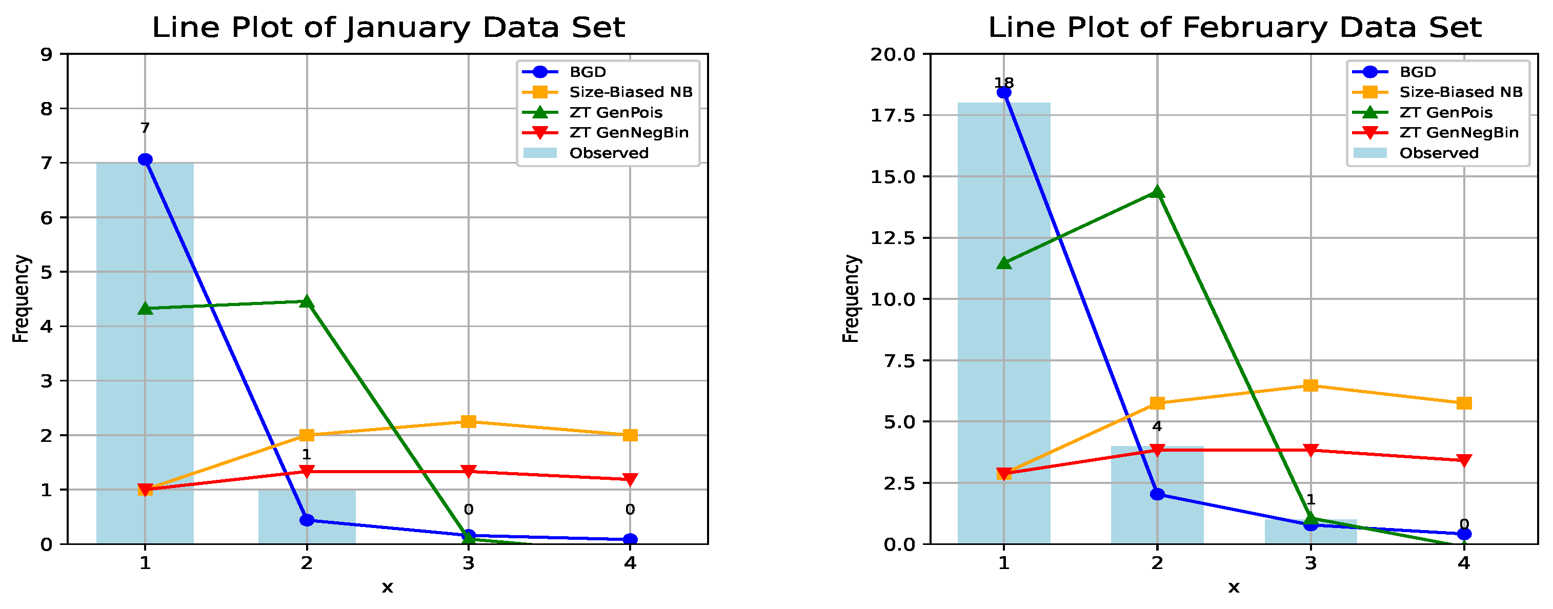
The BGD is the only model that consistently and adequately fits the data. In every table, its ${\chi }^2$ value is the lowest, and its p-value is well above the 0.05 significance threshold, ranging from 0.1545 to 0.4290. This indicates that the differences between its predicted frequencies and the actual observed data are small and statistically insignificant. For instance, in the first table for January thunderstorms, the BGD’s prediction of 7.06 events for x = 1 is almost identical to the observed frequency of 7, leading to an excellent fit.

In stark contrast, the other three models—SBNB, ZTGP, and ZTGNB—consistently and decisively fail to fit the data. All of them produce p-values of 0.0000 in every test, firmly rejecting the hypothesis that they are a good fit for these datasets. Their predicted frequencies are often wildly inaccurate. For example, the SBNB model predicts 9 thunderstorms for x = 1 in January when only 7 were observed, and a nonsensical 18 for x = 2 when only 1 was observed. Similarly, the ZTGP model severely over-predicts the frequency for x = 2 in multiple datasets. The ZTGNB model also fails dramatically, with χ² values that are often an order of magnitude larger than those of the BGD.

In conclusion, the results from the goodness-of-fit tests perfectly reinforce the findings from the AIC/BIC analysis. The BGD is unequivocally the superior model, demonstrating a statistically significant and accurate fit to the observed thunderstorm frequency data across all months. The other models are statistically invalid for this data, as their predictions consistently and significantly deviate from reality.

Interpretation Based on Vuong Statistics: The Vuong test is a statistical method used to compare non-nested models, assessing not only which model fits better but also whether the difference is statistically significant. The results across five datasets portrayed in

Table A3. Vuong Test Results for January Data Set.

Model 1	Model 2	Vuong Statistic	p-Value	Remarks
BGD	SBNB	32.1066	0.0000	GBD
BGD	ZTGP	0.3968	0.6915	No Decision
BGD	ZTGNB	4.1036	0.0000	GBD

,

Table A6. Vuong Test Results for February Data Set.

Model 1	Model 2	Vuong Statistic	p-Value	Remarks
BGD	SBNB	122.3449	0.0000	GBD
BGD	ZTGP	0.0895	0.6915	No Decision
BGD	ZTGNB	5.3326	0.0000	GBD

,

Table A9. Vuong Test Results for November Data Set.

Model 1	Model 2	Vuong Statistic	p-Value	Remarks
BGD	SBNB	76.3215	0.0000	BGD
BGD	ZTGP	0.4763	0.6335	No Decision
BGD	ZTGNB	5.6737	0.0000	BGD

,

Table A12. Vuong Test Results for December Data Set.

Model 1	Model 2	Vuong Statistic	p-Value	Remarks
BGD	SBNB	70.9318	0.0000	GBD
BGD	ZTGP	1.0636	0.6335	No Decision
BGD	ZTGNB	6.3391	0.0000	GBD

and

Table A15. Vuong Test Results for Winter Data Set.

Model 1	Model 2	Vuong Statistic	p-Value	Remarks
BGD	SBNB	NaN	0.0000	No Decision
BGD	ZTGP	0.8571	0.39	ZTGP
BGD	ZTGNB	8.7242	0.0000	GBD

reveal a consistent hierarchy of model performance. When comparing BGD to SBNB and ZTGNB, the test decisively favors BGD, with highly significant Vuong statistics (p-value = 0.0000), confirming that BGD’s fit is superior and that the negative binomial-based models are inferior for this data. In contrast, the comparison between BGD and ZTGP yields no significant difference, with high p-values (ranging from 0.39 to 0.69), indicating that both models are statistically equivalent in their fit. Consolidating all evidence—including AIC/BIC, goodness-of-fit tests, and the Vuong test—leads to the conclusion that SBNB and ZTGNB are definitively rejected, while the competition is primarily between BGD and ZTGP. Although BGD consistently performs slightly better, its advantage is not statistically significant, making ZTGP a viable and robust alternative. Overall, BGD is recommended as the optimal model due to its superior performance, but the non-significant difference with ZTGP highlights the latter’s validity as an equally plausible candidate.

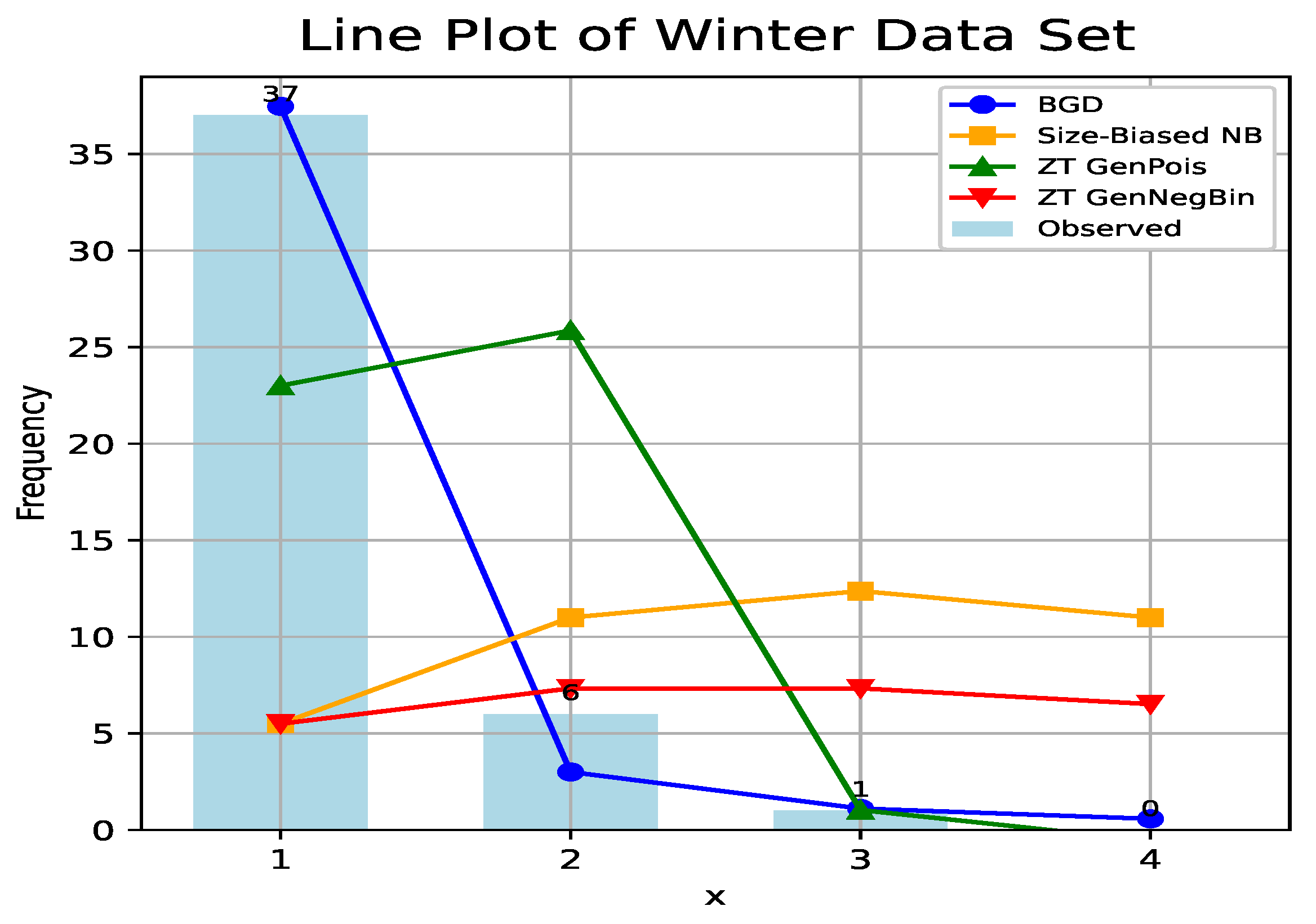
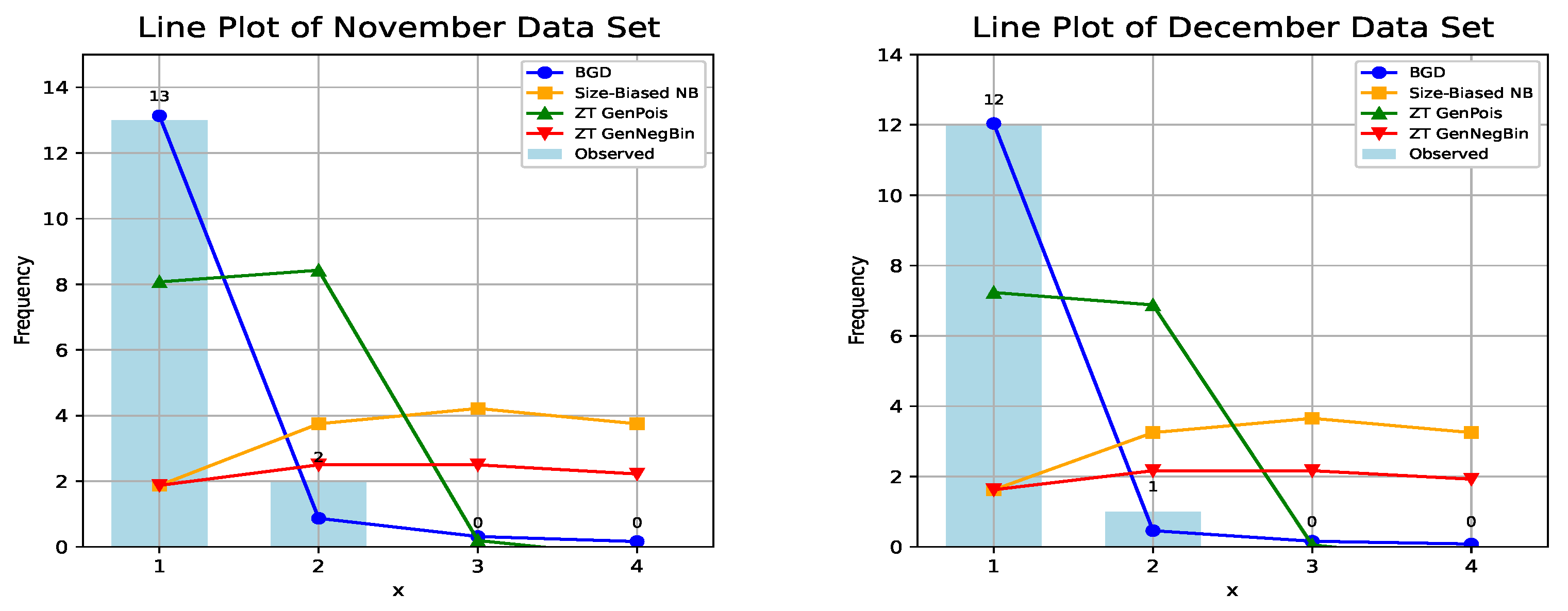
Interpretation Based on Plots: Figure A1, Figure A2 and Figure A3 likely depict the observed frequency of thunderstorm events against the predicted probabilities or frequencies from four models: BGD, ZTGP, SBNB, and ZTGNB. The key insight is a clear demonstration of model performance. The BGD line nearly perfectly follows the observed data points, especially at low values of x, capturing the rapid decay in frequency as x increases. The ZTGP line also aligns well with the data, though with slight deviations, consistent with its marginally worse AIC and the Vuong test’s “no decision.” In stark contrast, the SBNB and ZTGNB lines are severely misaligned, under-predicting at $x=1$ and over-predicting for higher x, with their lines remaining high while the actual frequencies approach zero. This misfit explains their large Chi-square values and insignificant p-values. Overall, these figures visually confirm that the BGD (and closely, the ZTGP) accurately model the underlying process, whereas the SBNB and ZTGNB models are inadequate for this thunderstorm frequency data.

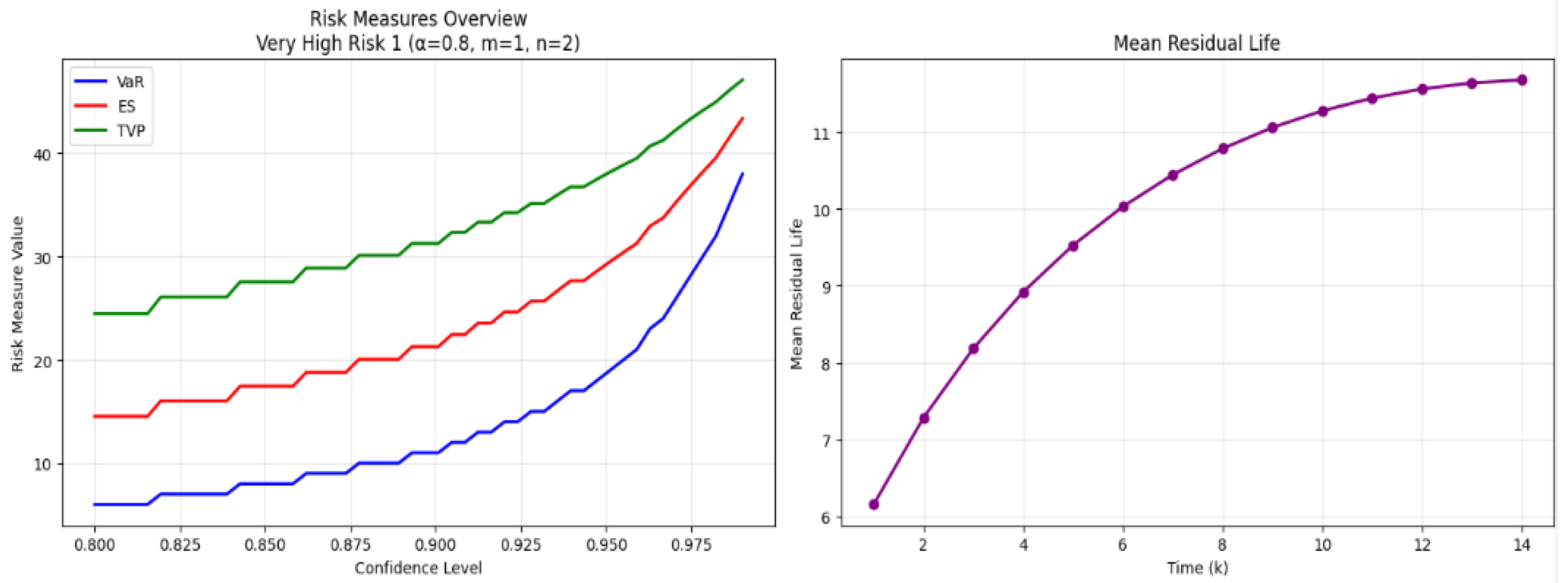
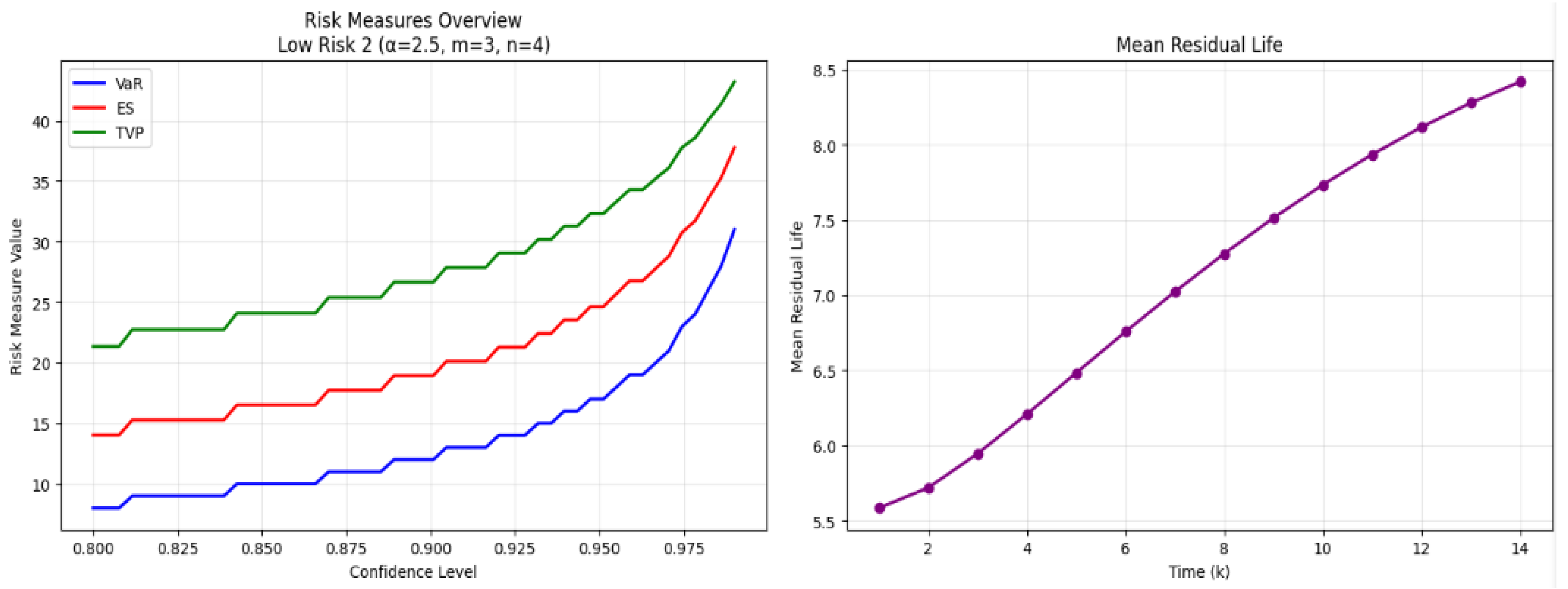
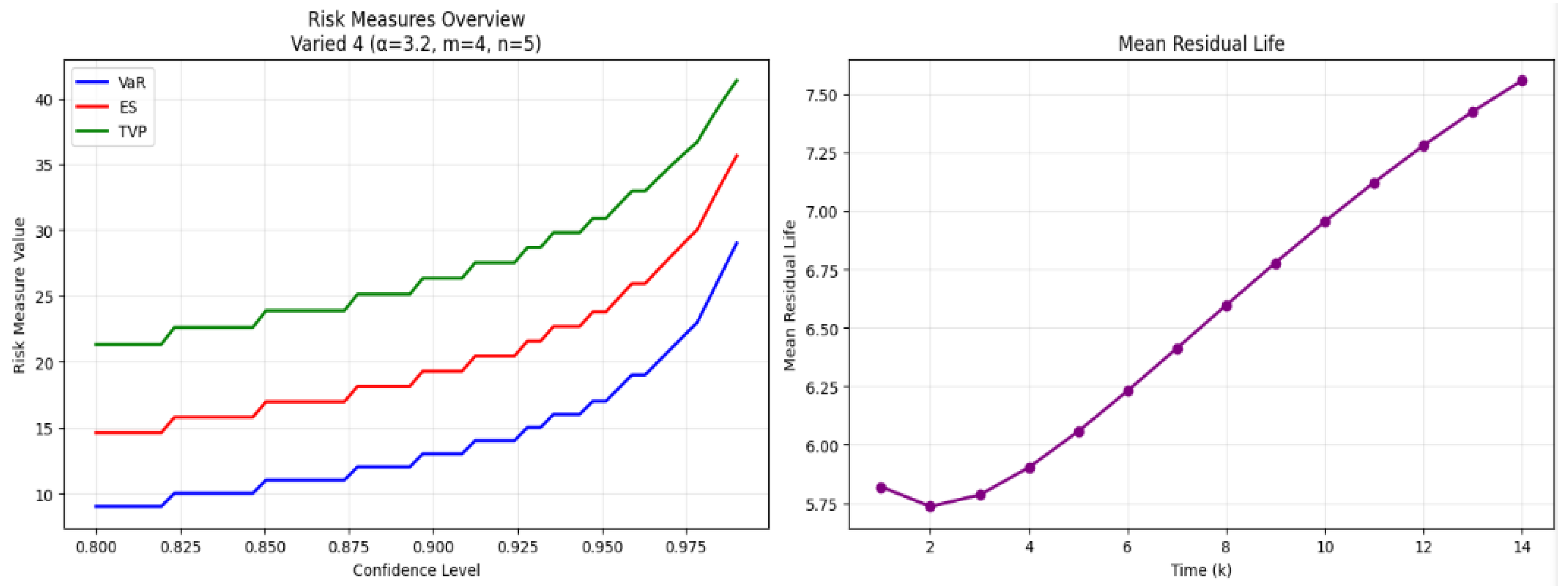
7.9. Risk Measure Results

Table 3. Comprehensive Comparative Risk Measures Summary for All Seasons.

Risk Measure	January	February	November	December	Winter
Mean (E[X])	1.0989	1.2226	1.21	1.1050	1.1651
VaR90%	1.0000	2.0000	2.00	1.0000	2.0000
VaR95%	2.0000	3.0000	2.00	2.0000	2.0000
VaR99%	3.0000	4.0000	3.00	3.0000	4.0000
ES90%	1.0989	2.4969	2.40	1.1050	2.4840
ES95%	2.2655	3.3445	2.40	2.3125	2.4840
ES99%	3.0000	4.0000	3.20	3.2500	4.0000
TVP90%	0.0989	0.4969	0.40	0.1050	0.4840
TVP95%	0.2655	0.3445	0.40	0.3125	0.4840
TVP99%	0.0000	0.0000	0.20	0.2500	0.0000
MRL(0)	1.0989	1.2226	1.21	1.1050	1.1651
MRL(1)	1.2655	1.4969	1.40	1.3125	1.4840
MRL(2)	1.0000	1.3445	1.20	1.2500	1.3432
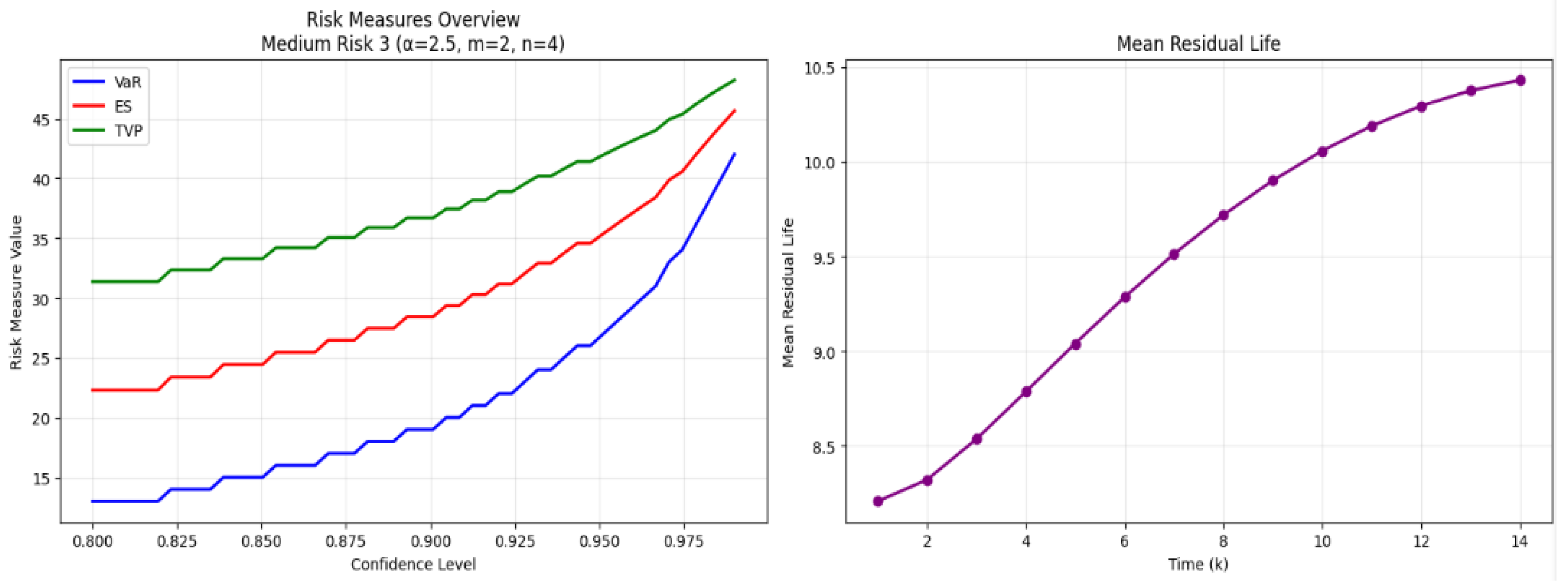
MRL(3)	–	1.0000	1.00	1.0000	1.0000

reveals distinct risk profiles across the winter months. The data indicates that February is the riskiest period, exhibiting the highest mean loss (1.2226), the highest Value at Risk (VaR) across all confidence levels, and the most severe ES. The significant disparity between February’s VaR_99% (2.0000) and its ES_99% (2.4969), quantified by a high Tail Value at Risk Premium (TVP_99% of 0.4969), signals a pronounced fat-tailed distribution where losses in the worst-case scenarios are substantially larger than the VaR threshold would suggest. This is further corroborated by the escalating MRL values; for instance, MRL(1) being much greater than MRL(0) indicates that once a threshold is exceeded, expected losses intensify considerably.

In contrast, January and December present a much milder risk environment, with lower mean losses, VaR, and ES. Their TVP values, particularly at the 99.9% level (0.0000), indicate that extreme losses are not significantly worse than the average, suggesting thinner tails. The overall Winter aggregate risk profile is heavily influenced by February’s severity, sitting between the riskiness of November and February. Consequently, a risk manager should prioritize February, employing the more conservative ES measure for capital allocation, as relying solely on VaR would underestimate the potential for severe, tail-risk events during this period.

7.9.1. Risk Level Assessment for January

Total thunderstorm days: 8. The average number of thunderstorms per event is 1.10. The 95% VaR indicates that up to two thunderstorms are expected with 95% confidence, while the worst-case scenario at the 99% VaR level suggests three thunderstorms. The expected shortfall at 95% is approximately 2.27 thunderstorms. Overall, the risk level is considered low, based on the 95% VaR of thunderstorms in January. Distribution characteristics show a 92.2% probability of experiencing exactly one thunderstorm, a 7.8% probability of two or more thunderstorms, and a 2.1% probability of three or more thunderstorms. The model quality assessments indicate that the BGD model has an excellent fit with a p-value of 0.3980, and an AIC difference of 0.227 provides moderate evidence in favor of BGD. The estimated parameters are $\alpha =0.133$, $m=1$, and $n=1$, with a very low variance of 0.1306 indicating high predictability. These findings have direct implications for launch operations and ground crew safety at KSC. For instance, the 95% VaR of two thunderstorms provides a statistically robust upper bound for baseline operations planning. Knowing that the probability of exceeding this threshold is only 5% allows mission planners to schedule critical, weather-sensitive activities with high confidence.

More importantly, the expected shortfall (ES) provides a conservative metric for contingency planning and resource allocation. For example, the ${\mathrm{ES}}_{95}$ of 2.48 thunderstorms indicates that, on the rare days where the 95% VaR is exceeded, one should expect an average of 2.48 storms. This insight is crucial for sizing emergency response teams, determining the duration of launch delays, and evaluating the financial risk of potential asset damage. The MRL function, which estimates the expected number of additional storms given that one has already occurred, offers real-time decision support. A high $\mathrm{MRL}\left(1\right)$ value would signal to forecasters that an ongoing event is likely to be complex and prolonged, warranting continued caution and potentially a decision to halt outdoor work or roll back sensitive hardware.

This information supports mission planning and risk management by providing reliable forecasts. In terms of risk quantification for insurance purposes, the expected loss frequency is approximately 1.099 events per occurrence, with a 99% worst-case scenario of 3 events. The risk premium, represented by the tail value at risk (TVP), is 0.265 additional events beyond VaR, indicating a well-defined and comprehensive tail risk quantification.

7.9.2. Risk Level Assessment for February

The risk assessment for February indicates a total of 23 thunderstorm days, with an average of 1.22 thunderstorms per event. The 95% VaR is three thunderstorms, and the worst-case scenario at 99% VaR is four thunderstorms, with an expected shortfall of 3.34 thunderstorms. The overall risk level is classified as medium, slightly higher than January but still manageable. Distribution characteristics show an 85.1% probability of a single thunderstorm and a 14.9% chance of multiple thunderstorms, with a small tail probability for four or more events. Model quality assessments favor the BGD model, which demonstrates a good fit and reasonable predictability, while the ZTGP model, despite a lower AIC, was rejected by goodness-of-fit tests. Compared to January, February exhibits a slightly higher mean frequency and a heavier tail, but both months maintain a low risk classification. Operationally, there is a high degree of predictability, with a maximum of three thunderstorms expected with 95% confidence, supporting effective mission planning and risk management.

7.9.3. Risk Level Assessment for November

The average number of thunderstorms in December is 1.21. The 95% value at risk (VaR) indicates that there are two thunderstorms, while the worst-case scenario at 99% VaR suggests up to three thunderstorms. The expected shortfall at 95% is 2.40 thunderstorms, reflecting the average number of thunderstorms exceeding the VaR threshold. Overall, the risk level for November is considered LOW, based on the 95% VaR of thunderstorms. Distribution characteristics show an 85.0% probability of exactly one thunderstorm, a 15.0% probability of two or more thunderstorms, and a 5.0% probability of three or more thunderstorms. Regarding model quality, the BGD model has a significantly lower AIC (20.8) compared to the next best model (22.4), with an AIC difference greater than two, indicating a substantially better fit. Additionally, the BGD parameters suggest a light-tailed distribution.

7.9.4. Risk Level Assessment in December

The average number of thunderstorms in December is 1.10. The 95% value at risk (VaR) indicates that there are two thunderstorms, while the worst-case scenario at 99% VaR suggests up to three thunderstorms. The expected shortfall at 95% is 2.31 thunderstorms, reflecting the average number of thunderstorms exceeding the VaR threshold. Overall, the risk level for December is considered LOW, based on the 95% VaR of thunderstorms. Distribution characteristics show a 92.0% probability of exactly one thunderstorm, a 8.0% probability of two or more thunderstorms, and a 2.0% probability of three or more thunderstorms. Regarding model quality, the BGD model has a significantly lower AIC (14.5) compared to ZTGP (19.3), with an AIC difference of 4.8, providing very strong evidence favoring BGD. Additionally, a very small $\alpha$ parameter (0.080) indicates a highly concentrated distribution. When comparing seasonally, December has the lowest mean (1.10) among all analyzed months, with the most concentrated distribution (92% probability of exactly one thunderstorm), and it exhibits the lowest tail risk and the most predictable pattern.

7.9.5. Risk Level Assessment-Winter

Total observations: in total, 44 thunderstorm days. The average number of thunderstorms per event is 1.17. The 95% VaR indicates that there are typically no more than two thunderstorms, while the worst-case scenario at 99% VaR is four thunderstorms. The expected shortfall at 95% is 2.48 thunderstorms. Overall, the risk level is considered LOW based on the 95% VaR of thunderstorms during winter, reflecting a relatively stable and predictable pattern.

The distribution characteristics reveal an 88.9% probability of experiencing exactly one thunderstorm, with a 11.1% chance of having two or more, a 4.0% chance of three or more, and a 1.4% chance of four or more thunderstorms. The model quality assessment shows that the BGD fits the data very well, with a p-value of 0.1545 and an AIC difference of 8.4, providing overwhelming evidence in favor of this model. The estimated parameters, $\alpha =0.174$, $m=1$, and $n=1$, suggest a light-tailed distribution that accurately captures the observed data.

Operationally, these findings imply that with 95% confidence, no more than two thunderstorms are expected during winter, and there is only an 11.1% probability of multiple thunderstorms occurring. This indicates a highly predictable pattern, making it suitable for mission planning purposes. The winter season exhibits a stable, low-risk thunderstorm pattern.

In a seasonal context, the winter mean of 1.17 thunderstorms aligns with the typical behavior observed in individual winter months. The distribution tends to concentrate at lower values, consistent with winter conditions. The BGD model continues to provide an excellent fit across all winter data, reinforcing the stability and low-risk nature of thunderstorms during this season.

8. Conclusions

This study successfully developed and presented the BGD distribution, a flexible compound distribution defined on the positive integers. The theoretical foundation of the BGD was thoroughly established, with explicit derivations of its fundamental properties, such as its probability mass function, moments, and reliability characteristics like the hazard rate and mean residual life functions. A significant contribution is the characterization theorem, which confirms the unique identifiability of the distribution through its characteristic function.

The hands-on dominance of the BGD was decisively confirmed through an empirical application. The model’s presentation establishes its crucial recompenses: its computational manipulability was established by the successful and stable convergence of parameter estimates across all datasets, a known encounter for the ZTGP. Its superior interpretability and sturdiness are reflected in its accurate fit without the systemic biases that can plague the misapplication of the SBNB.

The application to KSC thunderstorm data underscores a common scenario in risk analysis: the critical variable is often the severity of an event, given that it has occurred. The BGD distribution is uniquely suited for such contexts where the sample space is inherently conditioned on a positive count, providing a statistically sound and operationally relevant tool for conditional risk assessment.

Finally, its parameter parsimony prohibited the overfitting issues inherent to the more complex ZTGNB, resulting in a model that is both powerful and trustworthy for practical forecasting and risk assessment. Furthermore, it was the only model to consistently pass the Chi-square goodness-of-fit test, with high p-values confirming its predictions were not significantly different from the observed frequencies. While the Vuong test indicated that the BGD and the second-best model, the ZTGP, were statistically equivalent for these datasets, the BGD’s consistent edge in all other metrics solidifies its position as the recommended model. In summary, the BGD distribution proves to be a powerful and versatile tool for statistical modeling of positive count data. Its theoretical soundness, coupled with its demonstrated empirical performance in a critical real-world application, makes it a valuable addition to the statistician’s toolkit, particularly in fields like meteorology, reliability engineering, and risk and survival analyses where understanding the behavior of count processes that cannot be zero is essential.