Abstract
In a variety of applications, including signal processing, clock referencing, sensing, and others, microelectromechanical systems (MEMS) have been shown to be effective and broadly used. This study explores the dynamical response of a nonlinear MEMS resonator when subjected to a sudden mechanical shock under electrical excitation in the presence of quintic nonlinearity. The method of multiple scales (MMS) is utilized to construct the analytical formulas for analyzing the amplitude and phase response during primary resonance conditions. The analytical results are verified and compared with numerical simulations performed using the fourth-order Runge–Kutta method. Additionally, a parametric analysis is performed to examine the effect of different shock values on the resonator’s response and stability utilizing the Jacobian matrix. The agreement between analytical and numerical approaches proves MMS’s effectiveness in analyzing the shock impact on the MEMS resonator. The results provide valuable knowledge about the response and stability of MEMS resonators under mechanical shock, which is crucial for robust design in challenging conditions.
Keywords:
MEMS resonator; mechanical shock; frequency response; shock response; method of multiple scales; quintic nonlinearity MSC:
34C23; 34D10; 34D20; 34E13
1. Introduction
MEMS, or micro-electromechanical systems, have been an integral part of technological advancements in several fields over the past decades. MEMS devices are widely utilized as inertial sensors [1,2,3,4,5], micro-switches [6,7,8], biomass sensing [9,10,11], and resonators for different applications [12,13,14,15,16,17]. The reliability of MEMS devices when subjected to mechanical stress and impact during fabrication, shipping, or operation in harsh environments is a critical factor that must be considered and evaluated during the design process. Therefore, many researchers devote remarkable attention to studying the effect of the mechanical disturbance on MEMS devices [18,19,20].
The failure mode of MEMS suspended inductors is investigated by Yiyuan et al. [21] through the use of theoretical and experimental methodologies. This study identified critical stress as the failure criterion by combining the single degree of freedom (SDOF) model and solving a statically indeterminate structure. Stiction and electric short circuits occur when the vibrating beam makes contact with the fixed beam due to electrostatic force and mechanical stress. This contact causes pull-in instability, which is undesirable in many applications, which should be avoided to provide safe operation. Mechanical shock can produce early dynamic pull-in instability in microbeam structures due to unanticipated dynamic loading and impact.
For space applications, different designs of capacitive MEMS accelerometers were tested in [22] by Marozau et al. to identify the common failure causes and suggest an acceptable design. Lixin et al. [23] studied the Radio Frequency (RF) performance variation and failure scheme of a MEMS suspended inductor under high-g shock, with acceleration amplitudes as high as tens of thousands of g. The manufacturing process and air cannon impact testing were performed. The results indicated that the quality factor and inductance value of the inductors diminish to varying extents following shock exposure.
There has been a lot of interest in the analysis of electrically-actuated beams subjected to mechanical shock in recent years because it could provide guidance for designing robust MEMS devices with resistance to shock or investigate the possibility of using nonlinear phenomena for switching applications [15,24,25,26]. Jrad et al. [24] introduced a novel device consisting of an electrostatically actuated cantilever microbeam affixed to a tip mass and positioned atop a compliant board or printed circuit board. They constructed a mathematical model of the proposed device, demonstrating its significant tunability with variations in DC and AC voltages, as well as its capacity to detect a broad spectrum of acceleration (ranging from 0.33 to 200 g).
In [25], Wang et al. designed an inertial microswitch with a multi-directional compact constraint structure, which showed shock-resistance improvement. The simulation findings of ultra-high g acceleration (tens of thousands) in the reverse sensitive direction suggested a design of an inertial microswitch that can avoid false triggers. Igor et al. [26] introduced an analytical approach to construct the best ratio of parameters for specific applications. As an example, they created a design for an integrated RF MEMS switch that uses a capacitive switching principle, has low control voltages, a high switching speed, and is suitable for use in the X frequency range (8–12 GHz) in terrestrial and satellite radio communication devices.
The category of high-g MEMS devices, which are designed to be responsive to excessive shock levels (operating in the range of thousands of g), is frequently utilized in military applications [27,28,29,30]. Conversely, the performance of numerous electrically-actuated microsensors may be adversely impacted by mechanical stress [31,32,33]. To guarantee the dependability of these sensors, it is essential to mitigate mechanical shock effects by employing various designs that exhibit greater robustness to minimize dynamic pull-in. Ilyas et al. [34] successfully created and tested a new design of a resonator that is constructed out of dual cantilever microbeams that are electrically related to one another. The dynamic characteristics of the coupled microsystem offered potential for a variety of MEMS applications. In [35], Ahmed et al. simulated the dynamic responses of single and dual electrically actuated microbeams when subjected to mechanical shock. Their findings suggested the use of a dual-beam system in lower frequency ranges applications because it offered a reduction in both the static pull-in voltage and the switching time.
Fadi et al., in [36], considered the influence of printed circuit board (PCB) motion on the microstructure of MEMS devices subjected to varying shock pulse settings. The research revealed that inadequate PCB design may result in premature dynamic instability when subjected to shock loads. The research additionally showed that elevated vibration modes exert less influence on the microstructure’s reaction, unless their natural frequency is proximate to both the PCB and shock pulse frequency. In [37], Younis et al. examined the influence of mechanical shock and its effect time on an electrostatically driven resonator. The results showed that the resonator may fail as a result of its response being either amplified or weakened, and AC and DC loads needed to be taken into account for dependable MEMS resonator functioning.
Recent studies in nonlinear dynamics have revealed different approaches to enhance the stability and resilience of synchronized systems such as electrostatically coupled microscale oscillators and macroscale mechanically coupled rotors under disturbance conditions. Shi et al. [38] presented an approach demonstrating that white noise of appropriate intensity can enhance the stability of synchronized systems by diluting the energy of unwanted fluctuations from external disturbances, thereby preserving synchronization through the system’s inherent noise suppression at the synchronized frequency. Chen et al. [39] proposed a novel diamond honeycomb-like disk resonator gyroscope to enable operation under extremely high overload conditions by applying geometric shape refinement.
The necessity of incorporating quintic nonlinearity in the modeling of MEMS resonators has been firmly established through recent experimental and theoretical investigations. Liu et al. [40] demonstrated through parametrically excited MEMS micro-resonators that fifth-order nonlinearity is required to accurately describe the amplitude-frequency curves when parametric excitation strength exceeds certain thresholds. Their investigation and experimental findings of this work revealed an amplitude deflection phenomenon that occurs when parametric excitation strength surpasses critical values, which could only be explained by establishing a dynamic model incorporating fifth-order nonlinearity and nonlinear damping. This supports the inclusion of quintic terms in the present shock response analysis, as mechanical shock inherently introduces large transient amplitudes and strong excitation conditions that push the system beyond the cubic nonlinearity regime.
The dynamical response of a nonlinear MEMS resonator is investigated in this study. In the presence of quintic nonlinearity, the MEMS resonator is subjected to a rapid mechanical shock while simultaneously being electrically activated. To the best of our knowledge, this work represents the first systematic investigation of mechanical shock effects on electrostatically actuated MEMS resonators exhibiting quintic nonlinearity, which distinguishes it from previous studies that have primarily focused on cubic nonlinear models or static excitation conditions. When doing an analysis of the amplitude and phase response under primary resonance conditions, the method of multiple scales (MMS) is applied to create the analytical formulas that are necessary for the analysis. Using numerical simulations that are carried out with the fourth-order Runge–Kutta (RK4) method, the outcomes of the analysis are validated and contrasted with one another. Furthermore, this study presents novel insights into the electro-mechanical dynamics under transient shock loading, revealing previously unreported bifurcation phenomena and hysteretic behavior specific to quintic nonlinear systems. Using the Jacobian matrix, a parametric analysis is carried out in order to study the impact that different shock levels have on the responsiveness and stability of the resonator. The comprehensive parametric investigation systematically maps the basins of attraction and stability boundaries across varying detuning parameters and shock acceleration magnitudes, which provides new design guidelines for shock-resistant MEMS devices that leverage higher-order nonlinearities for enhanced sensitivity and multi-stable operation.
This paper is organized as follows: The clamped-clamped microbeam’s under the effect of mechanical shock mathematical modeling is examined in Section 2. The MEMS response equations to the electric stimulation in the presence of the mechanical shock are then obtained by applying perturbation analysis to the model in Section 3. Section 4 and Section 5 present the detailed results and discussion of frequency, shock responses and numerical simulations. Lastly, the article’s conclusions are summarized in Section 6.
2. Mathematical Modeling of MEMS Vibration Subject to a Mechanical Shock
Shock is a sudden force or impulse applied over a tiny time. This sudden application of force results in a rapid transmission of energy into the system, causing significant and often nonlinear changes in its mechanical state. When modeling the dynamic effects of mechanical shock on structural systems, several pulse shapes are utilized to approximate real-world shock profiles. Among these, the half-sine pulse is widely regarded as the most illustrative form due to its smooth curvature and close similarity to the actual shock experienced in physical systems. This shape offers a practical balance between mathematical simplicity and physical accuracy [41]. Consequently, the half-sine pulse, Figure 1, has become the standard in shock modeling across commercial, industrial, and military applications. In this study, the half-sine pulse form is adopted for the simulations as follows:
where is the shock duration and is the Heaviside step function.
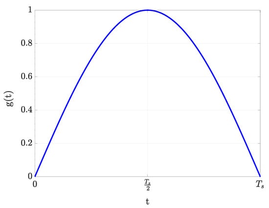
Figure 1.
Half-sine pulse used to model mechanical shock. This profile is commonly adopted in simulations due to its smooth curvature and resemblance to real-world shock conditions.
The nonlinear governing equation for the microbeam, which is subjected to both a DC voltage () and an AC voltage () with excitation frequency , as well as mechanical loading [35] (as illustrated in Figure 2), is given by:
where is the vertical deflection at any position and time , is the area moment of inertia, is its density, b is its width, h is its thickness, is the axial load, L is the beam’s length, d is the gap distance between the electrodes, m is the beam’s mass per unit length, E is Young’s modulus, c is the viscous damping coefficient, is the dielectric constant, f is the shock acceleration and A is the cross sectional area of the beam. The physical parameters utilised in the present model are derived from [42] and are outlined as follows. The beam material possesses a Young’s modulus and a density . The geometric dimensions of the microbeam are specified as a length , width , and thickness . The gap between the beam and the electrode is specified as .
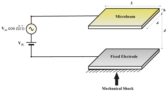
Figure 2.
Schematic of a clamped clamped MEMS resonator under mechanical shock.
The beam is subjected to the fixed-fixed boundary conditions:
To facilitate the analytical treatment and reduce the number of physical parameters, the governing equations are reformulated using the following set of non-dimensional variables:
where quantities denoted by a hat represent dimensional parameters, and the corresponding symbols without a hat denote their dimensionless counterparts. It is particularly noteworthy that the numerous design variables governing the system have been reduced to a small set of non-dimensional parameters by scaling the vertical displacement, time, and source frequency with the system’s characteristic quantities, such as gap distance, beam length, and natural frequency. One vital purpose of using the non-dimensional variables is comparing the system response amplitude to the gap distance, which helps identify the impact of the forcing variations on the system response. Moreover, using non-dimensional variables helps to generalize the characterization of systems rather than describing a specific system with particular specifications, thus avoiding divergence in computational processing. Upon applying this transformation, Equation (2) is cast into the dimensionless form:
where the parameter represents the dimensionless magnitude of the shock. The solution to Equation (5) is expressed as a combination of static and dynamic deflections. The static component is denoted by and the dynamic component is given by . The static component corresponds to the case where the transverse displacement does not vary with time.
Equation (6) is solved numerically using Algorithm 1 in [43]. Now, inserting into Equation (5),
Simplifying and multiplying both sides of Equation (7) by , yields
A further simplification is made to Equation (8) and the linear free vibration is obtained by dropping the forcing, damping and nonlinear terms.
Assuming a dynamic response of the form , where is the natural frequency and denotes the associated mode shape for the linear dynamic response, and substituting this expression into Equation (9), followed by applying the orthogonality condition of the mode shapes, yields
which characterizes the relationship between the natural frequency and the mode shape function in the presence of the DC component. The mode shape is numerically approximated using Algorithm 2, provided in Appendix A in [43]. For the nonlinear dynamic Equation (8) is discretized using the Galerkin method by assuming an approximate solution of the form . In the absence of internal resonance, and when the system operates near primary resonance conditions, a single-mode approximation is typically sufficient to capture the dominant dynamics [42]. This is because the first mode dominates the response under typical operating conditions, with the contribution of higher modes being relatively small. Therefore, focusing on one mode provides a clear understanding of the primary resonance characteristics and the onset of nonlinear phenomena such as amplitude jumps and bifurcations resulting from forcing variations. Substituting into Equation (8) results in
Here, and represent the spatial and temporal components of the dynamic deflection, respectively. By grouping like terms in Equation (11) and applying the orthogonality property of the mode shapes, the governing equation for the temporal function can be derived as follows:
where the dimensionless coefficients M’s are defined in Appendix A. Equation (12) features quintic nonlinearity resulting from the combined contributions of both higher-order geometric stretching effects and the nonlinear electrostatic forcing. The mid-plane stretching effect introduces a cubic nonlinearity related to geometric stiffening. Additionally, the electrostatic forcing shows second-order nonlinearity due to the inverse-square relationship between force and gap distance. The quintic nonlinearity arises from the multiplicative coupling of these two mechanisms, where the cubic geometric nonlinearity interacts with the quadratic electrostatic nonlinearity, leading to fifth-order terms in displacement.
3. Analytical Prediction of MEMS Response to Source Voltage and Mechanical Shock
To analyze the nonlinear dynamic behavior of a MEMS resonator subjected to both electrostatic excitation and external mechanical shock acceleration f, we apply the Method of Multiple Scales (MMS). MMS is a well-known method for solving equations with mixed quadratic, cubic, and higher-order nonlinear terms. It has been thoroughly tested in the nonlinear dynamics literature. The effectiveness of MMS for analyzing MEMS devices with mixed nonlinearities is shown in [44,45,46]. These studies developed extensive MMS-based analytical methodologies for systems with quadratic, cubic, and higher-order nonlinear terms, effectively forecasting intricate phenomena such as internal resonances, bifurcations, and hysteretic behavior, thereby validating its efficacy in managing multiple coexisting nonlinearities in electrostatically actuated MEMS devices. The goal is to derive the frequency response equation and perform a stability analysis via the Jacobian matrix. MMS is applied to derive an approximate analytical solution to Equation (12). This technique assumes that the solution can be expanded as a perturbation series in terms of a small bookkeeping parameter , yielding:
where the independent time scales are defined as , , and , corresponding to fast and slow temporal variations in the system response. The parameter is a small nondimensional quantity that reflects the strength of nonlinearity and the order of the perturbation expansion [47,48]. In Equation (13), denotes the zeroth-order approximation, capturing the dominant behavior of the system in the absence of perturbation effects. The term represents the first-order correction that incorporates the linear influence of the small perturbation parameter . Finally, is the second-order correction function, which accounts for higher-order nonlinear interactions or secondary effects induced by the perturbation.
To ensure that all essential system parameters, including damping, nonlinearity, and external forcing appear in the final frequency response expression, the relevant coefficients in the governing equation are perturbed accordingly [49]. This perturbation incorporates both even and odd-order nonlinearities and leads to an accurate understanding of how the system’s dynamic behavior is affected by quadratic, cubic, and higher-order terms. The scaling choice is selected to capture the physical dynamics of our electrostatically actuated MEMS resonator under shock excitation and is consistent with established practices for studying strongly nonlinear systems. Seminal and recent works [45,46,50,51,52,53] scaled the forcing terms as to achieve a balance between excitation, damping, and nonlinear effects at the same order. If the forcing were scaled at , it would overwhelm the nonlinear and damping effects, leading to a trivially dominated linear response that fails to capture the rich nonlinear phenomena including bifurcation, hysteresis, and amplitude jumps. After performing the necessary perturbations and substitutions, Equation (12) is reformulated as:
The function is approximated using Fourier approximation to take the form
The time derivatives transform according to the chain rule as:
where . In this study, the primary resonance is examined, where the detuning parameter indicates the degree to which the natural frequency differs from the source frequency. The zeroth-order equation is obtained by substituting Equation (13) into the governing nonlinear differential Equation (14) and collecting terms of ,
with the general solution:
where and are complex conjugate amplitude functions. The first-order equation is obtained at ,
Substituting Equation (18) into Equation (19) and eliminating secular terms imply that and are functions of z only; that is, . Accordingly, is obtained as follows:
The second-order equation is
By substituting A and B into Equation (21), eliminating the secular terms, and assuming and , where and represent the amplitude and phase of the resonator’s temporal displacement , respectively, we obtain the following system by separating the real and imaginary parts.
The amplitude-phase system given by Equations (22) and (23) is converted into an autonomous form by introducing the variable . The following system is the one obtained:
The steady-state operation is achieved at , where and ; under this condition, the following nonlinear frequency response equation of the MEMS resonator is obtained:
where are given in the Appendix A Equations (A7)–(A12). Considering the right-hand sides of Equations (24) and (25) as and , respectively, the local stability of the steady-state response is determined by computing the elements of the Jacobian matrix , which are the partial derivatives of the functions and as shown in the appendix Equation (A13). The eigenvalues of determine the stability regions. If the real parts of all eigenvalues are negative, the solution is stable. If any eigenvalue has a positive real part, the solution is unstable. The elements of Jacobian matrix are
4. Frequency and Shock Response Under Electrostatic and Mechanical Impact
This section investigates the frequency response Equation (26) of a MEMS resonator under moderate electrostatic excitation, where both the DC and AC voltages are set to along with mechanical shock of second, close around the resonator’s natural frequency, with natural period of and the computed parameters provided in the Appendix A. In this analysis, the applied shock duration is , it is evident that . This indicates that the shock event occurs on a timescale much shorter than the system’s characteristic dynamic response. Consequently, the shock acts effectively as an impulsive excitation to deliver a sudden burst of energy [41]. The structure does not reach steady state during the shock loading but instead undergoes a transient free vibration response following the impulse. This justifies modeling the shock as an instantaneous excitation when analyzing the subsequent dynamic behavior of the MEMS resonator. In all frequency and shock response figures, solid curves represent stable branches, while dashed curves indicate unstable ones.
Figure 3, Figure 4, Figure 5, Figure 6 and Figure 7 are derived from the analytical response using Equations (26)–(30) to study steady-state behaviors predicted analytically. Figure 3 and Figure 4 show the response amplitude is plotted as a function of the detuning parameter of the MEMS resonator under a constant DC and AC voltage of 5 V. The response of the resonator is depicted in the baseline Figure 3a, which is obtained without any mechanical shock being applied. One can plainly see the nonlinear behavior that is characteristic of the phenomenon, and a hysteresis behavior is present. The crucial locations for jump phenomena are defined by the stable and the unstable branches, and when rises, the system changes between a bistability and multi-stability states. In Figure 3a, when increases, the system evolves from a bi-stable configuration (two stable branches separated by an unstable one on left side) to a multi-stable regime with multiple coexisting steady states.
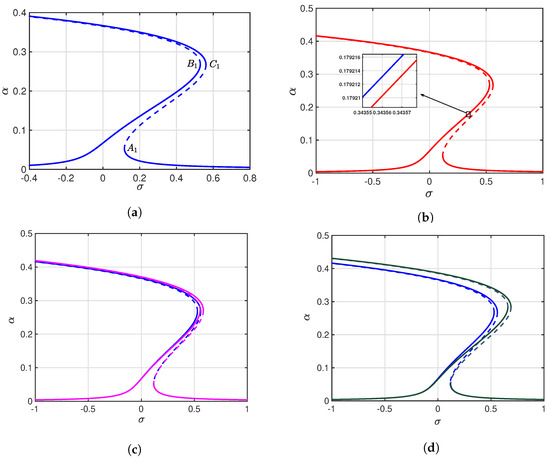
Figure 3.
Frequency response curves of the MEMS resonator at V for varying mechanical shock accelerations. (a) Frequency response at zero shock acceleration (blue). (b) Frequency response at 0 (blue) vs. 100 m/s2 shock (red). (c) Frequency response at 0 vs. m/s2 shock (magenta). (d) Frequency response at 0 vs. m/s2 shock (green).
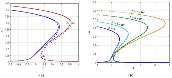
Figure 4.
Frequency response curves of the MEMS resonator at V. (a) Frequency response at 0 (blue) vs. m/s2 shock (brown). (b) Frequency response at 0 vs. various shock values.
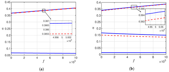
Figure 5.
The MEMS resonator’s shock response curves at V. (a) . (b) . The blue solid curves indicate stable branches, while the red dashed curves represent unstable ones.
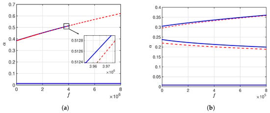
Figure 6.
The MEMS resonator’s shock response curves at V. (a) . (b) . The blue solid curves indicate stable branches, while the red dashed curves represent unstable ones. (The horizontal axis scale differs, about in (a) and in (b).)
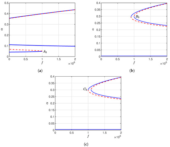
Figure 7.
Shock response curves of the MEMS resonator at V for various values. (a) . (b) . (c) . The blue solid curves indicate stable branches, while the red dashed curves represent unstable ones.
As shown in Figure 3 (before and after applying shock), the presence of three stable states in the electrostatically actuated MEMS resonator arises from the coupled effects of geometric midplane stretching and electrostatic nonlinearities, which generate quintic terms in the governing equations. Identifying bistable and multistable regions is vital for assessing the device’s safety margin against pull-in instability. At the saddle-node bifurcation points, the amplitudes along the stable branches must remain well below the normalized pull-in limit () to avoid electrode contact and device failure. When approaches , the resonator becomes prone to dynamic pull-in, while maintaining ensures safe and reliable operation within the multistable regime. Consequently, bifurcation analysis offers a practical means to define safe operating ranges that balance high sensitivity with structural stability under shock loading. Additionally, within the range of to , three saddle-node bifurcations occur, when a stable branch intersects with an unstable branch of solutions. One saddle-node bifurcation point is located on the left at , while two points and are situated on the right at and , respectively.
In Figure 3a, when the detuning parameter is forward swept from small values to higher ones, the amplitude response of the microbeam increases rapidly until reaching point . At this saddle-node bifurcation point, a jump occurs in the amplitude, transitioning either to the upper stable branch at or to the lower stable branch at . If the system jumps to the upper stable branch and continues to increase beyond point , a downward jump to the lower stable branch occurs. Conversely, during a backward frequency sweep where decreases past point , an upward jump to one of the upper stable branches at either or is produced.
In Figure 3b, with only a minor change in the peak amplitude and hysteresis boundaries, the response closely resembles the zero-shock curve at a comparatively small mechanical shock of 100 m/s2 (red). The slight bifurcation changes brought on by the weak perturbation are highlighted by the inset zoom. This indicates that the dynamic range and multi-stability of the resonator are slightly impacted by low value shocks.
Moving from Figure 3a–d, it can be noted that when the shock acceleration increases, the turning points locations are shown to be moved and the curve bending increases toward the right, indicating an enhancement of nonlinear behavior. In Figure 3c,d, the frequency response is slightly shifted to the right with the increase in f to m/s2 (magenta) and m/s2 (green), respectively. In addition, the frequency response curve exhibits an overall increase in the response amplitude which suggests that the shock input enhances the energy of the system. Furthermore, the left stable branch clearly stretches to the right, which means that the system can sustain higher oscillation amplitudes over a wider range of detuning values. Figure 4a reveals that the system responds very differently when the shock value is m/s2 (brown). The unstable branch moves to a more central area of the response curve as the hysteresis loop lengthens.
It is noted that the saddle-node bifurcations (at ), (at ) and (at ) emerge to right of the corresponding points , and . Figure 4b shows the response of the system under higher levels of shock acceleration f. As the value of f increases, some characteristics can be noted. Firstly, the stable branch spreads over a wider frequency range which indicate the resonator keep a wider stable operation. Additionally, overall increase in the amplitude which suggests providing the system with energy. Significantly, an upper unstable branch starts to appear when f reaches which emphasis the impact of the shock on changing the stability landscape of the resonator.
The shock response curves in Figure 5, Figure 6 and Figure 7 show the MEMS resonator response to a wide range of shock acceleration, for different values of the detuning parameter . In Figure 5a, the shock response is investigated at , where two stable branches are observed, divided by an unstable region in proximity to the upper stable branch. With a value of , Figure 5b displays multi-stable branches in addition to two unstable branches, one of which is located in close range to the upper stable branch. The insets in both Figure 5a,b can be used to confirm the value of at with the frequency response curve in Figure 3d.
In Figure 6a, where , the amplitude increases to higher levels as shock acceleration increases, compared to Figure 5a,b. At the same time, the unstable portion continues throughout a wide range of f, along with only one stable branch. This unstable part indicates that the resonator dynamics are significantly affected by the unstable solutions of the corresponding values of f. Figure 6b shows the presence of three stable branches alongside two unstable ones. The bottom stable branch remains nearly invariant with rising f, whereas the top stable branch progressively increases with f.
Figure 7 presents the shock response curves of the MEMS resonator operating at V over a wide range of shock acceleration frequencies for three detuning parameter values: , , and . For (Figure 7a), the upper branch demonstrates a gradual amplitude increase from approximately to as the shock acceleration increases, while the lower branch decreases slightly from to . In Figure 7b () demonstrates a bistability and multi-stability behaviors in the shock acceleration range –. Figure 7c () exhibits qualitatively similar behavior to the case, where a distinct jump from a stable equilibrium state to an unstable branch is clearly evident. When the value of is swept past any of saddle-node bifurcation point, the resonator response state changes qualitatively.
Figure 7a illustrates the shock response at , where a saddle-node bifurcation point is apparent at . This point corresponds to the saddle-node bifurcation point in Figure 4a at which increasing frequency sweep result in a jump in the response amplitude from to or on the far upper stable branch. Figure 7b depicts the shock response at , revealing a saddle-node bifurcation point at . The point corresponds to the saddle-node bifurcation point in Figure 4a, where frequency forward sweep makes jumps from up to or down to on the lower stable branch. In Figure 7c, the saddle-node bifurcation point corresponds to the point in Figure 4a, where increasing frequency sweep results in a jump in the response amplitude from to on the lower stable branch. None of the response amplitude values that result from the sudden jumps approach unity, which is the crucial value for pull-in instability. This means that the system stays away from the dynamic pull-in condition and indicates higher resistance to the mechanical shock.
5. Time-Response and Phase Plane Analysis
The dynamic behavior of the MEMS resonator is shown in Figure 8, Figure 9, Figure 10 and Figure 11, with a constant actuation voltage of V, and changing shock acceleration f and detuning parameter by applying RK4 on Equation (12). These results display the necessity to know what makes shock loading and frequency detuning interact to affect stability of the system, transient dynamics, and steady-state response.
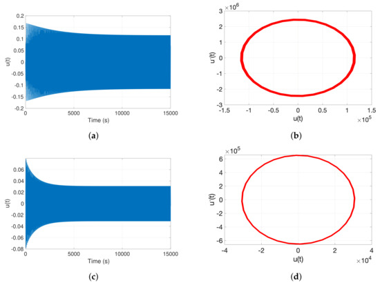
Figure 8.
Time response and phase-plane (u, ) plots of the MEMS resonator at V, zero initial conditions for varying . (a,b) ; (c,d) ; all at .
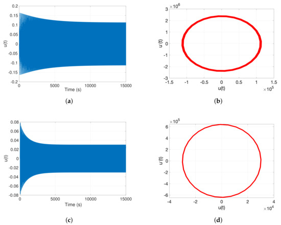
Figure 9.
Time response and phase-plane (u, ) plots of the MEMS resonator at V, zero initial conditions for varying . (a,b) ; (c,d) ; all at .
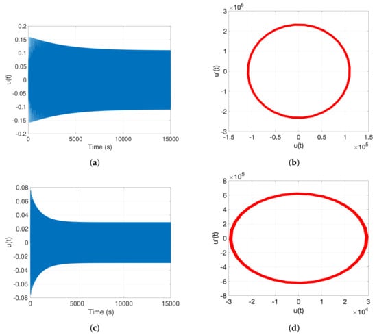
Figure 10.
Time response and phase-plane (u, ) plots of the MEMS resonator at V, zero initial conditions for varying . (a,b) ; (c,d) ; all at .
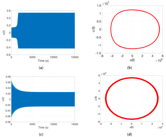
Figure 11.
Time response and phase-plane (u, ) plots of the MEMS resonator at V, zero initial conditions for varying . (a,b) ; (c,d) ; all at .
Figure 8 and Figure 9 illustrate the dynamic response of the MEMS resonator at two different shock acceleration levels, and , for narrowly spaced detuning values. At the lower shock acceleration of (Figure 8), Figure 8a,b show that for , the resonator exhibits a relatively large response amplitude and slow convergence toward the steady-state, indicating prolonged transient behavior. The corresponding phase plane trajectory forms a large elliptical orbit, reflecting high oscillatory energy. A slight increase in detuning to (Figure 8c,d) leads to a significant reduction in amplitude and a quicker stabilization, as well as a noticeably smaller elliptical orbit in the phase plane.
A similar trend is observed under a higher shock level of (Figure 9). For (Figure 9a,b), the system demonstrates pronounced oscillatory motion and a gradual approach to steady-state, with a large phase portrait loop indicating elevated dynamic energy. Increasing the detuning slightly to (Figure 9c,d) results in a markedly diminished amplitude and rapid convergence, with a corresponding phase portrait that is more compact. The comparison across both shock levels reveals consistent sensitivity of the resonator’s dynamics to minor detuning variations near resonance. Minor variations in result in significant alterations in amplitude and convergence properties at elevated shock accelerations, when this sensitivity becomes more pronounced.
Figure 10 and Figure 11 show the MEMS resonator’s time-domain and phase-plane responses under higher shock accelerations. In Figure 10, corresponding to , the time response for (Figure 10a,b) exhibits a moderately large amplitude with relatively slow decay. The associated phase portrait confirms this behavior with a wide elliptical trajectory. However, when is increased slightly to (Figure 10c,d), the response amplitude decreases sharply, and convergence to steady-state is much faster. The corresponding phase plane exhibits a compact and stable orbit, further indicating energy reduction.
In contrast, Figure 11 examines a significantly larger shock acceleration of . For , the system exhibits a very large amplitude response (Figure 11a), characterized by a slow and complex transient regime with delayed convergence. The phase portrait (Figure 11b) shows a large, slightly distorted elliptical orbit, signaling strong nonlinear dynamics. Interestingly, a minor increase in to (Figure 11c,d) leads to a substantial suppression of oscillation amplitude and a highly compact, rapidly decaying response, both in the time domain and the phase plane. The comparison of Figure 10 and Figure 11 underscores a consistent trend: at elevated shock levels, the system remains highly sensitive to small perturbations in the detuning parameter. Nevertheless, the nonlinearities become more pronounced at higher shocks, as seen in the more distorted orbits and stronger oscillatory responses. These results indicate the role of fine-tuning in regulating the dynamic stability and energy dissipation of MEMS resonators under harsh shock environments.
To provide quantitative validation of our analytical MMS predictions against numerical RK4 simulations, the Root Mean Square (RMS) error has been calculated across multiple parameter configurations. For the amplitude responses presented in Figure 3c and Figure 8a,c, at detuning parameters and under shock acceleration , the calculated RMS error is 0.24%. For the amplitude responses shown in Figure 4a and Figure 10a,c, at detuning parameters and under shock acceleration , the RMS error is 0.07%. This excellent agreement demonstrates the high accuracy of the MMS approach in the moderate shock regime where perturbation assumptions remain valid. For the amplitude responses depicted in Figure 4b and Figure 11a,c, at detuning parameters and under shock acceleration , the RMS error increases to 3.2%. While still within acceptable engineering tolerance, this elevated error reflects the approaching validity boundary of the perturbation expansion at high shock magnitudes. The applicability range of our analytical approach is defined by the shock magnitude. The MMS predictions maintain high accuracy (RMS error ) for shock accelerations up to , as shown in Figure 4b. Beyond this threshold, particularly when (RMS error = 3.2%), accuracy deteriorates due to the transient dynamic effects, and potential higher-mode excitation.
Equations (24) and (25) are used to determine the system response state plane for various shock accelerations f and . In Figure 12, Figure 13, Figure 14 and Figure 15, the MEMS resonator system’s state plane portraits (, ) are shown at and without and with a variety of mechanical shock excitation. The figures show the nonlinear dynamics and how the amplitude and phase change over time from different initial conditions. In all cases, the driving voltages of the MEMS are .
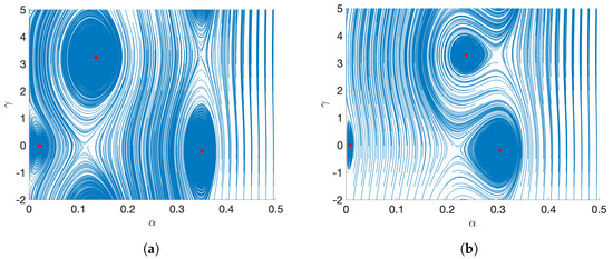
Figure 12.
The MEMS resonator’s state plane curves at V for zero shock acceleration. (a) . (b) .
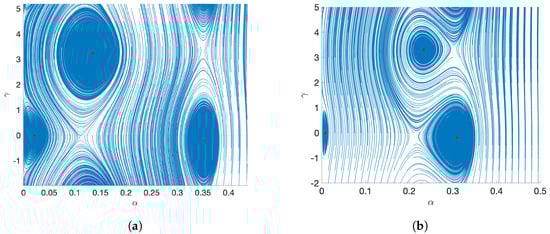
Figure 13.
The MEMS resonator’s state plane at V for shock acceleration . (a) . (b) .
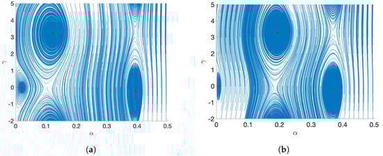
Figure 14.
The MEMS resonator’s state plane at V for shock acceleration . (a) . (b) .
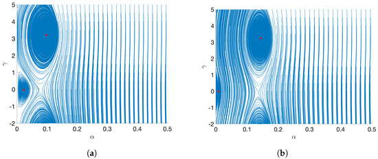
Figure 15.
The MEMS resonator’s state plane at V for shock acceleration . (a) . (b) .
In Figure 12, which shows the scenario of no mechanical shock (), the system acts in a conventional nonlinear way, with steady-state responses and clear zones of attraction. The trajectories show how the system changes from different initial conditions to its steady-state response. As seen in Figure 12a,b, three distinct stable spiral points (small red ones) are present. Depending on initial conditions, low-amplitude, medium-amplitude and high- amplitude steady-state develop. In Figure 3a, at the detuning parameter value , the amplitude response exhibits three distinct equilibrium states corresponding to , , and . These three amplitude values represent stable fixed points of the system, as evidenced by their appearance as attractors (red points) in the phase plane portrait presented in Figure 12a. The phase plane analysis reveals that each of these equilibrium amplitudes is associated with its own basin of attraction, delineated by the concentric contour patterns surrounding each red point. Trajectories initiating within a particular basin will converge to the corresponding attractor, demonstrating the multistable nature of the system at this detuning value. The coexistence of these three stable equilibrium states explains the complex amplitude-frequency relationship observed in Figure 3a, where the system can settle into different oscillation amplitudes depending on the initial conditions. In Figure 12b, for , a notable deformation in the geometry of the state plane is shown which indicates response sensitivity to the detuning parameter .
In Figure 13a, low-amplitude, medium-amplitude and high- amplitude steady-state oscillations present near , and , respectively. A saddle point exists between them, forming separatrices that divide the domains of attraction. The spiral trajectories signify eventual decay towards a spiral point based on initial conditions. At , , the state plane shown in Figure 13b reveals the existence of three steady-state: a low-amplitude steady-state at approximately , a medium-amplitude steady-state at , and a high-amplitude steady-state occur at . These results match the amplitude levels shown in the shock response in Figure 6b.
At the higher mechanical shock level , as illustrated in Figure 14, the state-plane trajectories for both detuning values become more orderly and symmetric compared to lower shock levels. When the shock acceleration is extremely high, denoted as , as seen in Figure 15, the system displays two spiral points at low-amplitude steady-stat. When the value of is reached, the trajectories become thin vertical bands. On the other hand, when the value of is reached, the state plane exhibits prominent vertical features with lateral spread which suggests that the dynamics of the resonator in this case become shock-dominated.
6. Conclusions
This study explored the dynamic behavior of a clamped-clamped MEMS resonator under the impact of a mechanical shock in the presence of nonlinearities ranging from quadratic to quintic order. The beam was actuated by both AC and DC electric fields and was modeled to include the effects of axial loading and mid-plane stretching. To analyze the system near primary resonance, the method of multiple scales was employed to derive approximate analytical solutions for the amplitude and phase of the response. Stability characteristics were examined using a Jacobian matrix-based approach, which provided the criteria for identifying stable and unstable operating regions. A series of response curves were generated at various shock accelerations f and detuning parameter to illustrate the system’s behavior under varying operational parameters. The results showed that the MEMS resonator kept working normally when it was subjected to different levels of mechanical shock. It was able to resist disturbances and continue to work within its typical dynamic range which is a crucial characteristic for practical MEMS applications requiring reliability in adverse environments. The system showed nonlinear behavior which was clear in the frequency-response characteristics. The frequency-response and shock response graphs showed a noticeable jump in the response amplitude , along with areas of bistability and multi-stability. These nonlinear properties suggest that the system has complicated dynamic behavior, which indicates that is has more than one steady-state solution at the same time. The system kept stable oscillations at the saddle-node bifurcation sites on the frequency-response and state plane graphs. In addition, the system’s time-response and phase-plane exhibit a consistent sensitivity to slight detuning adjustments around resonance at elevated shock accelerations. Nevertheless, at increased shock levels, the system exhibits significant sensitivity to minor changes in the detuning parameter. The nonlinearities intensify with increased shocks, evidenced by increasingly deformed orbits and heightened oscillatory responses.
Moreover, the system’s response to shock changed from initial conditions to a steady-state, exhibiting three separate stable spiral points. The state plane displayed low-amplitude (), medium-amplitude (), and high-amplitude () steady-states dependent upon initial conditions and the detuning parameter . In addition, the response sensitivity to the detuning parameter was apparent in the geometry of the state plane. At elevated shock levels, the state plane trajectories exhibited increased order and symmetry. When the shock acceleration was excessively high, the system showed two spiral points at low-amplitude steady-state. Finally, future research should focus on performing experimental studies to validate the theoretical predictions drawn from this work. The empirical investigations provide deeper knowledge about the practical implementation challenges, fabrication tolerances, and real-world nonlinear behavior under coupled electrostatic and mechanical disturbances. Additionally, exploring the effects of temperature variations, material imperfections, and environmental disturbances could further enhance the reliability and applicability of MEMS resonators in advanced sensing and actuation systems.
Author Contributions
Conceptualization, A.K.; Methodology, A.K.; Software, M.E.A.; Validation, M.E.A., K.M. and A.K.; Formal analysis, A.K.; Investigation, M.E.A. and A.K.; Writing—original draft, M.E.A.; Writing—review & editing, A.E., K.M., W.K.Z. and A.K.; Supervision, A.E., W.K.Z. and A.K. All authors have read and agreed to the published version of the manuscript.
Funding
This research work is supported by the Egyptian Ministry of Higher Education (MOHE) in the scope of the Egypt-Japan University of Science and Technology(E-JUST).
Data Availability Statement
The original contributions presented in this study are included in the article. Further inquiries can be directed to the corresponding authors.
Conflicts of Interest
The authors declared that there are no conflicts of interest related to the research, authorship, and/or publication of this article.
References
- Ghommem, M.; Nayfeh, A.H.; Choura, S. Model reduction and analysis of a vibrating beam microgyroscope. J. Vib. Control 2013, 19, 1240–1249. [Google Scholar] [CrossRef]
- Mo, Y.; Du, L.; Qu, B.; Peng, B.; Yang, J. Squeeze film air damping ratio analysis of a silicon capacitive micromechanical accelerometer. Microsyst. Technol. 2018, 24, 1089–1095. [Google Scholar] [CrossRef]
- Peng, T.; You, Z. Reliability of mems in shock environments: 2000–2020. Micromachines 2021, 12, 1275. [Google Scholar] [CrossRef] [PubMed]
- Ru, X.; Gu, N.; Shang, H.; Zhang, H. Mems inertial sensor calibration technology: Current status and future trends. Micromachines 2022, 13, 879. [Google Scholar] [CrossRef]
- Al Jlailaty, H.; Celik, A.; Mansour, M.M.; Eltawil, A.M. Imu hand calibration for low-cost mems inertial sensors. IEEE Trans. Instrum. Meas. 2023, 72, 1–16. [Google Scholar] [CrossRef]
- Cao, T.; Hu, T.; Zhao, Y. Research status and development trend of mems switches: A review. Micromachines 2020, 11, 694. [Google Scholar] [CrossRef]
- Du, L.; Yang, X.; Guo, B.; Dong, Y.; Yuan, B.; Zhao, J.; Liu, J. A novel mems inertial switch with frictional electrode. J. Micromech. Microeng. 2022, 32, 065008. [Google Scholar] [CrossRef]
- Kurmendra; Agarwal, S. Mems switch realities: Addressing challenges and pioneering solutions. Micromachines 2024, 15, 556. [Google Scholar] [CrossRef]
- SoltanRezaee, M.; Bodaghi, M. Simulation of an electrically actuated cantilever as a novel biosensor. Sci. Rep. 2020, 10, 3385. [Google Scholar] [CrossRef]
- Mansoorzare, H.; Shahraini, S.; Todi, A.; Azim, N.; Rajaraman, S.; Abdolvand, R. Liquid-loaded piezo-silicon micro-disc oscillators for pico-scale bio-mass sensing. J. Microelectromech. Syst. 2020, 29, 1083–1086. [Google Scholar] [CrossRef]
- Deshwal, D.; Narwal, A.K. Analysis of surface deviation impact on bio-mass sensing application of boron nitride nanotubes. Results Eng. 2023, 19, 101282. [Google Scholar] [CrossRef]
- Zhang, C.; Jiang, W.; Ghosh, A.; Wang, G.; Wu, F.; Zhang, H. Miniaturized langasite mems micro-cantilever beam structured resonator for high temperature gas sensing. Smart Mater. Struct. 2020, 29, 055002. [Google Scholar] [CrossRef]
- Pillai, G.; Li, S.-S. Piezoelectric mems resonators: A review. IEEE Sens. J. 2020, 21, 12589–12605. [Google Scholar] [CrossRef]
- Colombo, L.; Kochhar, A.; Vidal-Alvarez, G.; Piazza, G. High-figure-of-merit x-cut lithium niobate mems resonators operating around 50 mhz for large passive voltage amplification in radio frequency applications. IEEE Trans. Ultrason. Ferroelectr. Freq. Control 2020, 67, 1392–1402. [Google Scholar] [CrossRef]
- Kurmendra; Kumar, R. A review on rf micro-electro-mechanical-systems (mems) switch for radio frequency applications. Microsyst. Technol. 2021, 27, 2525–2542. [Google Scholar] [CrossRef]
- Abdelraouf, M.E.; Kandil, A.; Zahra, W.K.; Elsaid, A. Investigation of a mems resonator model with quintic nonlinearity. In Journal of Physics: Conference Series; IOP Publishing: Bristol, UK, 2024; Volume 2793, p. 012019. [Google Scholar]
- Zhao, H.; Chen, X.; Xin, C.; Zhao, F.; Cheng, S.; Lei, M.; Wang, C.; Zhang, J.; Chen, X.; Tian, H.; et al. High-sensitivity and self-powered flexible pressure sensor based on multi-scale structured piezoelectric composite. Chem. Eng. J. 2025, 519, 164787. [Google Scholar] [CrossRef]
- Qiao, Y.; Xu, W.; Sun, J.; Zhang, H. Reliability of electrostatically actuated mems resonators to random mass disturbance. Mech. Syst. Signal Process. 2019, 121, 711–724. [Google Scholar] [CrossRef]
- Peng, B.; Hu, K.-M.; Fang, X.-Y.; Li, X.-Y.; Zhang, W.-M. Modal characteristics of coupled mems resonator array under the effect of residual stress. Sens. Actuators A Phys. 2022, 333, 113236. [Google Scholar] [CrossRef]
- Gasparin, E.; Hoogerwerf, A.; Bayat, D.; Durante, G.S.; Petremand, Y.; Tormen, M.; Despont, M.; Close, G. An integrated mems magnetic gradiometer rejecting vibrations and stray fields. In Proceedings of the 2024 IEEE European Solid-State Electronics Research Conference (ESSERC), Bruges, Belgium, 9–12 September 2014; pp. 532–535. [Google Scholar]
- Li, Y.; Li, J.; Xu, L. Failure mode analysis of mems suspended inductors under mechanical shock. Microelectron. Reliab. 2018, 85, 38–48. [Google Scholar] [CrossRef]
- Marozau, I.; Auchlin, M.; Pejchal, V.; Souchon, F.; Vogel, D.; Lahti, M.; Saillen, N.; Sereda, O. Reliability assessment and failure mode analysis of mems accelerometers for space applications. Microelectron. Reliab. 2018, 88, 846–854. [Google Scholar] [CrossRef]
- Xu, L.; Li, Y.; Li, J. Analysis of the failure and performance variation mechanism of mems suspended inductors with auxiliary pillars under high-g shock. Micromachines 2020, 11, 957. [Google Scholar] [CrossRef]
- Jrad, M.; I Younis, M.; Najar, F. Modeling and design of an electrically actuated resonant microswitch. J. Vib. Control 2016, 22, 559–569. [Google Scholar] [CrossRef]
- Xu, Q.; Yang, Z.; Sun, Y.; Lai, L.; Jin, Z.; Ding, G.; Zhao, X.; Yao, J.; Wang, J. Shock-resistibility of mems-based inertial microswitch under reverse directional ultra-high g acceleration for iot applications. Sci. Rep. 2017, 7, 45512. [Google Scholar] [CrossRef]
- Lysenko, I.E.; Tkachenko, A.V.; Sherova, E.V.; Nikitin, A.V. Analytical approach in the development of rf mems switches. Electronics 2018, 7, 415. [Google Scholar] [CrossRef]
- Parkos, D.; Raghunathan, N.; Venkattraman, A.; Sanborn, B.; Chen, W.; Peroulis, D.; Alexeenko, A. Near-contact gas damping and dynamic response of high-g mems accelerometer beams. J. Microelectromech. Syst. 2013, 22, 1089–1099. [Google Scholar] [CrossRef]
- Zhao, Y.; Li, X.; Liang, J.; Jiang, Z. Design, fabrication and experiment of a mems piezoresistive high-g accelerometer. J. Mech. Sci. Technol. 2013, 27, 831–836. [Google Scholar] [CrossRef]
- Shi, Y.; Zhao, Y.; Feng, H.; Cao, H.; Tang, J.; Li, J.; Zhao, R.; Liu, J. Design, fabrication and calibration of a high-g mems accelerometer. Sens. Actuators A Phys. 2018, 279, 733–742. [Google Scholar] [CrossRef]
- Holm, R.; Petersen, H.; Normann, S.; Schou, H.; Horntvedt, M.; Hage, M.; Martinsen, S. High–g (20,000 g+) testing of an existing tactical grade gyro design. In Proceedings of the 2020 DGON Inertial Sensors and Systems (ISS), Braunschweig, Germany, 15–16 September 2000; pp. 1–10. [Google Scholar]
- Srikar, V.; Senturia, S. The reliability of microelectromechanical systems (mems) in shock environments. J. Microelectromech. Syst. 2002, 11, 206–214. [Google Scholar] [CrossRef]
- Sundaram, S.; Tormen, M.; Timotijevic, B.; Lockhart, R.; Overstolz, T.; Stanley, R.P.; Shea, H.R. Vibration and shock reliability of mems: Modeling and experimental validation. J. Micromech. Microeng. 2011, 21, 045022. [Google Scholar] [CrossRef]
- Ouakad, H.M. The response of a micro-electro-mechanical system (mems) cantilever-paddle gas sensor to mechanical shock loads. J. Vib. Control 2015, 21, 2739–2754. [Google Scholar] [CrossRef]
- Ilyas, S.; Chappanda, K.N.; Al Hafiz, A.; Ramini, A.; Younis, M.I. An experimental and theoretical investigation of electrostatically coupled cantilever microbeams. Sens. Actuators A Phys. 2016, 247, 368–378. [Google Scholar] [CrossRef]
- Ahmed, M.S.; Ghommem, M.; Abdelkefi, A. Nonlinear analysis and characteristics of electrically-coupled microbeams under mechanical shock. Microsyst. Technol. 2019, 25, 829–843. [Google Scholar] [CrossRef]
- Alsaleem, F.M.; Younis, M.I.; Ibrahim, M.I. A study for the effect of the pcb motion on the dynamics of mems devices under mechanical shock. J. Microelectromech. Syst. 2009, 18, 597–609. [Google Scholar] [CrossRef]
- I Ibrahim, M.; I Younis, M. The dynamic response of electrostatically driven resonators under mechanical shock. J. Micromech. Microeng. 2009, 20, 025006. [Google Scholar] [CrossRef]
- Shi, Z.; Lv, Q.; Fu, M.; Wang, X.; Huang, Z.; Wei, X.; Amabili, M.; Huan, R. Noise-enhanced stability in synchronized systems. Sci. Adv. 2025, 11, eadx1338. [Google Scholar] [CrossRef]
- Chen, H.; Wu, K.; Li, Q.; Xiao, D.; Wu, X. Design method for mode matching of a novel diamond honeycomb-like disk resonator gyroscope with high shock resistance. In Journal of Physics: Conference Series; IOP Publishing: Bristol, UK, 2025; Volume 2982, p. 012025. [Google Scholar]
- Liu, Z.; Xu, Y.; Lv, Q.; Wang, X.; Chen, Y.; Dai, H.; Wei, X.; Huan, R. Amplitude deflection in a nonlinear mems resonator under parametric excitation. Int. J. Non-Linear Mech. 2024, 163, 104754. [Google Scholar] [CrossRef]
- Younis, M.I. MEMS Linear and Nonlinear Statics and Dynamics; Springer Science & Business Media: New York, NY, USA, 2011; Volume 20. [Google Scholar]
- Rocha, R.T.; Alfosail, F.; Zhao, W.; Younis, M.I.; Masri, S.F. Nonparametric identification of a micro-electromechanical resonator. Mech. Syst. Signal Process. 2021, 161, 107932. [Google Scholar] [CrossRef]
- Abdelraouf, M.E.; Kandil, A.; Zahra, W.K.; Elsaid, A. Analyzing mems resonator static pull-in and dynamics under electric excitation via position feedback controller. Phys. Scr. 2024, 100, 0152a2. [Google Scholar] [CrossRef]
- Zhao, J.; Sun, R.; Kacem, N.; Lyu, M.; Liu, P. Multi-channel mass sensing based on multiple internal resonances in three electrostatically coupled resonators. Nonlinear Dyn. 2023, 111, 18861–18884. [Google Scholar] [CrossRef]
- Nayfeh, A.H.; Mook, D.T. Nonlinear Oscillations; John Wiley & Sons: New York, NY, USA, 2024. [Google Scholar]
- Wu, J.; Song, P.; Zang, S.; Li, L.; Zhang, W.; Shao, L. Limit cycle convergence leads to period-doubling and cyclic-fold bifurcation in internal resonance-induced mechanical frequency combs. Nonlinear Dyn. 2025, 113, 19289–19310. [Google Scholar] [CrossRef]
- Francis, A.C.; Zahra, W.K.; Elsaid, A.; Kandil, A. Improvement of the non-periodic energy harvesting behavior of a non-ideal magnetic levitation system utilizing internal resonance. J. Vib. Eng. Technol. 2024, 12, 8363–8382. [Google Scholar] [CrossRef]
- Ibrahim, M.M.M.; Kandil, A.; Zahra, W.K.; Elsaid, A. Elimination of the vibration center shift in the nonlinear oscillations of a maglev vehicle subjected to steady and unsteady aerodynamic forces: Second-order multiple scales analysis. ZAMM-J. Appl. Math. Mech./Z. Angew. Math. Mech. 2025, 105, e70125. [Google Scholar] [CrossRef]
- Nayfeh, A.H. Introduction to Perturbation Techniques; John Wiley & Sons: New York, NY, USA, 2011. [Google Scholar]
- Younis, M.I.; Nayfeh, A.H. A study of the nonlinear response of a resonant microbeam to an electric actuation. Nonlinear Dyn. 2003, 31, 91–117. [Google Scholar] [CrossRef]
- Alsaleem, F.M.; I Younis, M.; Ouakad, H.M. On the nonlinear resonances and dynamic pull-in of electrostatically actuated resonators. J. Micromech. Microeng. 2009, 19, 045013. [Google Scholar] [CrossRef]
- Sun, R.; Zhao, J.; Kacem, N.; Dong, Z.; Song, J.; Liu, P. A new sensitivity enhancement scheme for resonant mass sensors based on 2: 1 internal resonance bifurcation topology tuning. Nonlinear Dyn. 2025, 113, 11193–11214. [Google Scholar] [CrossRef]
- Zamanzadeh, M.; Ouakad, H.M.; Azizi, S. Theoretical and experimental investigations of the primary and parametric resonances in repulsive force based mems actuators. Sens. Actuators A Phys. 2020, 303, 111635. [Google Scholar] [CrossRef]
Disclaimer/Publisher’s Note: The statements, opinions and data contained in all publications are solely those of the individual author(s) and contributor(s) and not of MDPI and/or the editor(s). MDPI and/or the editor(s) disclaim responsibility for any injury to people or property resulting from any ideas, methods, instructions or products referred to in the content. |
© 2025 by the authors. Licensee MDPI, Basel, Switzerland. This article is an open access article distributed under the terms and conditions of the Creative Commons Attribution (CC BY) license (https://creativecommons.org/licenses/by/4.0/).