1. Introduction
As the demographic factor, captured by the dependency ratio, is the driving force behind upward expenditure trends [
1], many countries that traditionally avoided funded pensions are now incorporating these into their main pillars. One example is Greece, which established its first fully funded pension fund in the first pensions pillar in 2021. Looking at developed countries as a whole, ref. [
2] discusses how many OECD (Organisation for Economic Co-operation and Development) countries have undertaken pension reforms to address pension and aging-related challenges. These reforms often include raising the retirement age, adjusting benefit formulas, and promoting private pension schemes to complement public pensions. Additionally, the report notes the importance of adapting pension systems to demographic changes to ensure that they remain both adequate and financially viable. On the other hand, many countries have been retracting privatization reforms and have returned to more traditional, Pay-as-you-go Pension Plan (PAYG) systems [
3]. In total, eighteen countries, thirteen in Eastern Europe and the former Soviet Union and five in Latin America, reversed privatizations, meaning 60 per cent of the countries that had privatized pensions reversed the process and started to switch back to public systems [
4].
The replacement rate has long been a key consideration in pension planning, reflecting how effectively a pension system can replace a retiree’s pre-retirement earnings. This metric is invaluable for both policymakers and pension planners, serving as a foundational tool to design systems that balance adequate retirement income with the sustainability of the pension framework [
5]. Therefore, replacement rate helps determine if retirees will be able to sustain their standard of living after they stop working. A higher replacement rate indicates a pension system that provides greater financial security for retirees, offering a more comfortable standard of living during retirement. In contrast, a lower replacement rate may signal potential economic difficulties for retirees, raising concerns about the adequacy of their retirement income.
Given the complexity and dynamic nature of pension systems, there is a growing need for advanced tools that can accurately estimate and predict replacement rates. Recent actuarial studies have shown that deep learning can effectively model complex demographic and financial relationships, particularly in mortality forecasting and longevity risk estimation [
6]. These developments demonstrate that AI techniques are increasingly capable of addressing dynamic, non-linear pension-related phenomena, motivating their use in this study.
While replacement rates can be calculated deterministically from known inputs, real-world applications often involve uncertainty, incomplete data, or multi-pillar interactions where deterministic formulas alone may be insufficient. Techniques rooted in Artificial Intelligence (AI) and Decision Sciences, such as neural networks [
7] and fuzzy logic [
8], offer robust solutions to these challenges. Furthermore, explainable AI methods are gaining importance in actuarial and financial modeling, as they enable transparency and trust in predictive systems [
9]. This aspect is particularly relevant in pension planning, where interpretability supports regulatory compliance and stakeholder confidence.
In the context of pension planning, AI tools can play a pivotal role in (i) analyzing extensive datasets, (ii) identifying intricate patterns, (iii) developing decision-support tools, and (iv) delivering highly accurate predictions. For instance, these tools can provide preliminary replacement rate estimates, particularly in scenarios involving large-scale data analysis, enabling experts to make well-informed decisions based on data-driven insights. Even in scenarios where deterministic calculations exist, AI provides a scalable approach for integrating expert knowledge, handling large datasets, and supporting preliminary decision-making, enabling pension experts to focus on nuanced or multi-criteria adjustments.
This study investigates two innovative approaches for estimating replacement rates: (i) Artificial Neural Networks (ANNs) and (ii) a Fuzzy Inference System (FIS). Using a synthetic dataset, it evaluates the predictive capabilities of these AI-driven methods in comparison to traditional calculation techniques. These calculations take into account factors such as annuity values, contribution rates, and expected return rates. For both ANNs and FIS, the study explores various parameter configurations, aiming to identify optimal setups based on insights from previous research [
10]. Furthermore, to leverage the complementary strengths of ANNs and FIS, this study introduces a conceptual integration using the Analytic Hierarchy Process (AHP). This multi-criteria decision-making framework enables the systematic combination of the predictive accuracy of neural networks with the interpretability of fuzzy systems.
The novelty of this research does not lie merely in approximating deterministic outputs but also in demonstrating how AI can serve as a decision-support system, offering flexible, extensible, and scalable tools that can adapt to more complex or uncertain pension scenarios. This study therefore fills a gap in the literature by providing the first comparative assessment of ANN and Mamdani FIS models for replacement-rate estimation under a controlled experimental framework.
This work aligns with recent advances in hybrid AI systems that combine neural and fuzzy reasoning to achieve interpretable and adaptive decision-making frameworks [
11], further underscoring the potential of explainable intelligence in financial forecasting contexts. Particularly, this research lies in demonstrating how neural networks and fuzzy logic can enhance the precision and reliability of replacement rate estimations, offering significant improvements over conventional methods and paving the way for more effective pension management strategies.
The remainder of this paper is structured as follows:
Section 2 provides a brief literature review on the introduction of funded schemes internationally and the relevance of the latter to the promotion of savings and potential growth, as well as the application of AI techniques in pension modeling. In the following section (
Section 3), the methodology and all necessary equations together with the corresponding parameters are discussed. Moreover, the section outlines the methodology employed in this study, detailing the use of synthetic datasets and the implementation of neural networks and FIS for replacement rate calculations.
Section 4 presents computational experiments and results, including computer specification, data generation processes and results for both AI methods and traditional calculations. In addition to this, we analyze and discuss the results obtained from our experiments, highlighting the performance of neural networks and FIS compared to conventional approaches. Finally,
Section 5 concludes the paper with a summary of key findings and their implications for the future of pension planning. Moreover, it outlines future research directions, suggesting potential enhancements and expansions of the proposed methodologies. Additional details on the fundamental concepts of neural networks and fuzzy logic are provided in
Appendix A and
Appendix B, respectively.
2. Literature Review
Some countries decided to introduce mandatory fully funded pension schemes, as a second tier to the PAYG tier. Recent developments have led policy makers to recognize that fully funded components can be an integral part of an adequate retirement income. In this direction, several countries, including Sweden and some Eastern Member States such as Bulgaria, Estonia, Croatia, Latvia, Lithuania, Poland and Slovakia, and Sweden have switched part of their public pension schemes into (quasi-) mandatory private funded schemes [
1]. These arrangements are typically statutory, but the insurance relationship is between the individual and the pension fund. As a result, insured individuals retain ownership of their pension assets, allowing them to benefit from the returns but also assume the associated risks.
The introduction of funded pillars became popular across Europe after the 1990’s [
12], however, the reversals which followed the 2008 economic and financial crisis actually reduced or completely eliminated the role of funding in many countries [
13]. There were also serious disagreements about the effect of these privatizations [
4].
One of the main arguments in favor of funded schemes is that they promote growth. Based on the econometric results found in [
14], it can be confirmed that the investments of pension funds have had a positive impact on the economic growth of selected non-OECD countries. It is found that the strong performance of pension funds from 2002 to 2018 directly boosted the economies of non-OECD countries. Increased funds available for pension asset investments led to improved efficiency in their capital markets, fueling economic growth.
For OECD countries, a recent study by the OECD [
2] likewise stresses the importance of private pensions to economic growth. The underlying logic is that larger pension assets can translate into greater investment, which in turn can fuel economic activity and growth. OECD also shows that pension fund assets in the OECD area exceeded USD 35 trillion at end-2020, versus 32.3 in 2019 [
15]. There was an increasing trend despite COVID-19 in almost all countries except those facing significant early withdrawals.
Having said that, let there be no doubt that funded schemes, as PAYG schemes, also come with flaws. In 2018, a study of the International Labour Organization (ILO) presented an extensive list of these flaws, as perceived by its authors [
4]. Examples are the stagnation of coverage rates, the deterioration of pension benefits, the increase in gender and income inequality, the high transition costs and respective large fiscal pressures, high administrative costs, weak governance, the concentration of the private insurance industry, the actual benefits and their recipients, the actual effect on capital markets in developing countries, the transfer of financial markets and demographic risks from states to individuals and the deteriorated social dialogue.
In any case, the typology of the pension funds around the world shows an increase in funded pensions systems and an overall inclination of countries to implement these [
1,
2], without this meaning that negative aspects of funded schemes are neglected.
It is worth mentioning that the field of pension systems and aging populations has witnessed significant progress, largely driven by the integration of machine learning and advanced statistical techniques. Research reviewed in this survey highlights a wide range of applications for these methodologies, covering various aspects of pension management and elderly care. Recent studies demonstrate that deep learning techniques, such as Long Short-Term Memory (LSTM) models, have been successfully applied to mortality forecasting in developing countries, highlighting their potential for actuarial applications in pension systems [
16]. In parallel, AI-driven portfolio optimization has proven valuable for managing pension fund assets, supporting both individual and institutional investment decisions [
17].
Liu et al. (2024) [
18] conducted a study aimed at predicting osteoporotic fractures using Electronic Health Records (EHR). Their work tested 12 machine learning algorithms and 3 hybrid models, focusing on identifying risk factors. The top-performing model combined Support Vector Machine (SVM) with XGBoost, achieving over 90% accuracy and highlighting key clinical variables. In another study, ref. [
19] applied survival analysis techniques to Turkey’s private pension system, utilizing Cox regression, accelerated failure time models, and machine learning methods. Their findings show that machine learning provides non-parametric alternatives to traditional models, revealing socio-economic disparities in private pension participation.
In Hungary, the research by [
20] compared the effectiveness of (LSTM) neural networks with the traditional Lee-Carter model for mortality forecasting. Their findings showed that LSTM models achieved higher accuracy, underscoring their potential to enhance actuarial calculations and contribute to the sustainability of pension systems. Similarly, ref. [
21] examined the link between income-expenditure balance and retirement age in pension systems through machine learning techniques. Their analysis revealed a strong correlation between retirement age and life expectancy, offering important insights to guide policy decisions for creating sustainable pension schemes.
In Denmark, ref. [
22] employed statistical regularization and group bridge methods to analyze retirement transitions in the country’s pension programs, identifying significant factors that influence retirement decisions. Expanding on the evaluation of pension services, ref. [
23] introduced a novel method for assessing service quality by utilizing multi-dimension attention Convolutional Neural Networks (MACNN). The proposed method integrated emoticons, sentiment analysis, and textual features to provide deeper and more accurate insights into consumer sentiment compared to traditional methods.
Further advancing the role of AI technology, ref. [
24] addressed gaps in smart home pension systems by combining machine learning with wireless sensor networks. The proposed combination improved elderly care services by providing detailed data-driven insights into daily routines and health status. Additionally, ref. [
25] developed a machine learning algorithm specifically designed to model lexicographic preferences in decision-making. Applied to occupational pension schemes, this approach effectively supported decision-making by evaluating multiple attributes simultaneously.
In the field of public policy, researchers have also made significant contributions by advocating for Fuzzy Set Qualitative Comparative Analysis (FSQCA) as a valuable alternative to traditional case-oriented and regression-based methods. This method is particularly effective for research designs with smaller sample sizes, offering concise results while addressing the complexity of individual cases [
26].
Fuzzy decision-making methods have recently been extended to pension fund management and identification of medical insurance fraud, enabling adaptive strategies for risk assessment and asset/resource allocation [
27,
28]. Moreover, hybrid architectures that combine neural networks with fuzzy inference systems (ANFIS) have been explored to enhance prediction accuracy while maintaining interpretability, reflecting contemporary trends in AI-driven financial modeling [
29]. It should be noted that few studies on hybrid AI architectures have explored formal multi-criteria decision-making frameworks to systematically integrate the outputs of neural networks and fuzzy inference systems. This gap is particularly evident in pension planning, where balancing predictive accuracy with interpretability and expert knowledge is critical. Our study addresses this limitation by introducing AHP, providing a structured methodology to combine complementary AI approaches into a coherent decision-support framework.
Although numerous qualitative and quantitative studies have advanced the understanding of pension systems, a notable gap remains in the application of neural networks and fuzzy logic to replacement-rate estimation. Systematic reviews of fuzzy set applications in finance mostly emphasize their broad utility in risk management and decision-making [
30]. Moreover, few studies have adopted a comparative framework that incorporates explainable models such as fuzzy inference systems. This gap highlights the novelty and significance of exploring these methodologies further.
It is worth mentioning that while deterministic formulas exist for replacement rate estimation, they are often rigid and do not easily accommodate uncertainty, large-scale data, or multi-criteria considerations. The application of AI approaches such as neural networks and fuzzy logic provides scalable, adaptable, and extensible frameworks that can serve both as accurate predictors and as decision-support tools. This flexibility underscores the practical relevance of our study beyond simple function approximation.
3. Methodology
In this study, we aim to provide a controlled comparative evaluation of two alternative AI methodologies, Neural Networks (NNs) and Mamdani FIS, for estimating replacement rates in funded pension schemes. The selected variables, including annuity, contribution rate, return rate, total working years, and expected life of the annuity, are standard and theoretically grounded determinants in pension modeling [
10], capturing the key factors affecting replacement rate outcomes. The use of a large synthetic dataset allows precise benchmarking against exact calculations while ensuring diverse and realistic scenarios. While some linear relationships exist in the data, both AI methods are fully extensible to non-linear, stochastic, or real-world datasets. The models are intentionally presented independently as alternative approaches rather than hybridized, enabling a clear comparison of their respective strengths, limitations, and applicability for decision support.
In addition to separately modeling replacement rates using NN and FIS approaches, the study conceptually explores their potential integration through a multi-criteria decision-making framework based on the AHP, as described in
Section 3.6.
3.1. Overview of the Replacement Rate Concept
This paper will follow and showcase the three parameters mentioned above, as these are presented and analyzed in [
10]. These parameters are annuity, return on investment and contribution rate. In funded systems, a contributor puts aside a certain amount of money per period of time; in the end of their working life, they get back the accumulated funds. These comprise the future present value of the amounts paid, increased by the return on investment, and paid out in the form of a lifelong pension flow (annuity).
A simplified formula describing the accrued amount would be:
where:
: is the accrued amount at retirement;
X: is the amount of contributions per year (assumed fixed);
i: is the yearly rate of return on investment;
n: is the number of years of contribution.
3.1.1. The Baseline Scenario Analysis
As stated earlier, this paper will use the same baseline as in [
10] and build up the examples with neural networks and fuzzy logic, respectively. We will, however, mention the most essential points of the scenario to avoid extensive need of reference to the original text.
In a fully funded system that is implemented de novo, without any financial burden from past commitments. The potential transition from an already existing system, which is many times the case, along with its financial burden, is not analyzed in this paper. As in all pensions, the single most critical indicator is the projected replacement rate at the time of retirement. The replacement rate is defined as the fraction of the first pension amount, over the last wage. An alternative not used in this paper, substitutes the denominator with the average career income instead of the last wage.
In order to calculate representative replacement rates for the fully funded system, we expand Equation (1) to account for income variability and maturity. This allows us to calculate the required contribution rate as a percentage of a specific amount of income (e.g., 6% on earnings). We also account for a percentage of expenses on contributions. In this context, the accrued amount at time
n shall be given by:
where:
: is the accrued amount at time n;
: is the amount of contributions at time n as a percentage of income, before expenses;
E: is the percentage of expenses on contributions;
i: is the yearly rate of return on investment;
n: is the number of years of contributions.
The annual return rate on investment (i) is assumed to be constant for the purpose of simplicity. This means we practically use an average return rate overall instead of the different yearly rates. Payments are assumed monthly; hence, the amount of the last year is multiplied by as if there were one payment in the middle of the year, to simplify.
Let us use Equation (2) and proceed to calculate the replacement rate for a proposed funded scheme. To do that, certain additional assumptions are needed. These are the salary maturity per year (i.e., the percentage of increase in a person’s salary due to legislated increase based on more years of work, an increase in pay or a promotion), a baseline contribution rate which would serve as a norm or as the minimum (i.e., legislators are expected to present people with a standard percentage of contribution to either begin with or serve as the standard where choice is not made), an expense rate on contributions, and a real return rate (deducing expenses).
After careful considerations [
10], the full career is assumed to be 40 years, annuity is set to 15.64, the baseline contribution rate on pensionable earnings is set at 6% of pensionable earnings, maturity per year on income and expense rates on contributions are both set at 0.5% (see
Table 1). Finally, the real return rate (RRR) is carefully looked into [
10] using historical returns of 100 years along with experience from literature, OECD and EU publications, and the 30-year maturity of the Zero-coupon yield curve spot rates of AAA-rated euro area central government bonds and the whole euro area central governments bonds, and is set at 3.5% for the baseline, ranging from 2% to 6% for the sensitivity scenarios.
Using these assumptions, we calculate the replacement rate at 26.02% for 40 years or 0.65% yearly, which constitutes the baseline calculation.
We observe that the replacement rate covers a significant amount of return on retirement, with a contribution of 6% on pensionable income.
3.1.2. Sensitivity Analysis
In the previous subsection, a careful selection of assumptions was made in order to depict the baseline scenario. Drawing on research from [
10] we will now present the variations/sensitivity analysis for the three variables chosen, annuity, contribution, and return rate, respectively.
Based on different life tables and adjustments for the increase in life expectancy in the last years, ignoring the COVID-19 years which could lead to a serious miscalculation, we derive a span of 14.00 to 18.00, with a 0.1 interval. The replacement rates arising from the main annuity values can be found in
Table 2.
Respectively, we may assume values for the return rate varying between 2% and 6% based on extensive analysis and careful consideration of historical returns, experience from literature, publications of international institutions, and government bonds. Under these considerations, the baseline was set at 3.5%, while the sensitivity scenarios will range from 2% to 6%. Using a step of 0.1%, the results for the main values of the return rate and respective replacement rates are depicted in
Table 3 below.
Finally, the contribution rate is presented using values between 5% and 9%, based mainly on European experience. A step of 0.1% has been used.
Table 4 below shows the main contribution rate values and respective replacement rates.
3.2. Computational Methodology Overview
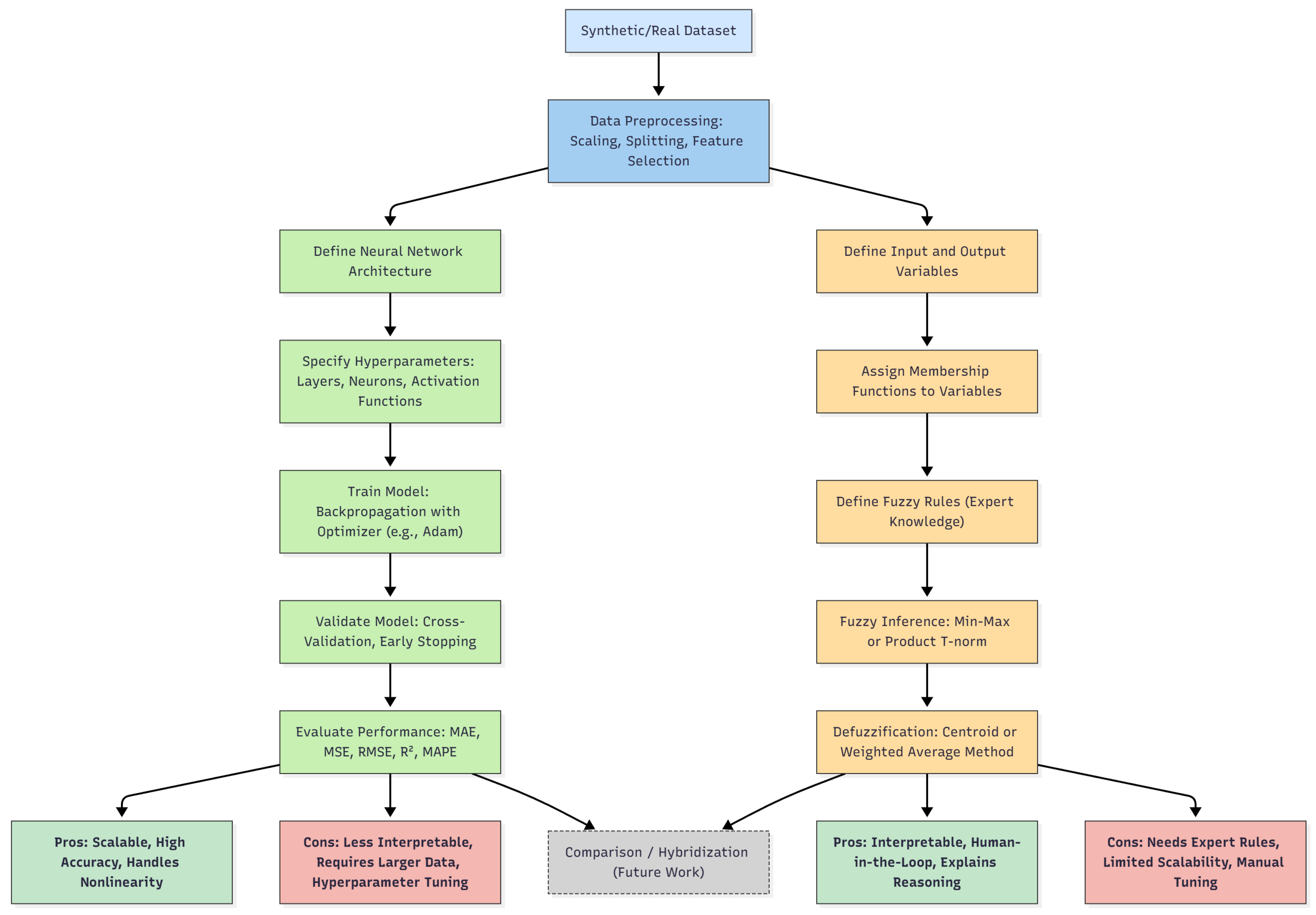
The computational methodology for estimating replacement rates in pension systems is designed as a structured pipeline that transforms raw inputs into predictive outputs through well-defined algorithmic steps. This framework aims to formalize the sequence of data preprocessing, model training, inference, and evaluation, allowing a rigorous understanding of the procedures while providing reproducibility and transparency.
The methodology can be conceptualized as a set of complementary toolboxes. The first toolbox is a neural network-based approach, where parameters are estimated through optimization over training data. This method is fully data-driven and suitable for high-dimensional problems. The second toolbox is a Mamdani FIS, which is human-in-the-loop and rule-based, enabling interpretable predictions without the need for iterative training. Both toolboxes share the same input space but differ fundamentally in the way knowledge is incorporated and outputs are generated. The combination of these two frameworks provides a versatile and rigorous computational environment for replacement rate estimation, allowing analysts to select the appropriate method based on data availability, interpretability requirements, and computational resources.
Figure 1 presents a schematic overview of the computational methodology developed in this study. The diagram illustrates two complementary analytical pipelines built upon a shared preprocessing stage. The lower section of the figure also highlights the comparative strengths and limitations of each method, as well as their potential hybridization for future research.
3.2.1. Mathematical Formalization of the Neural Network Pipeline
Let the dataset be denoted by:
where
represents the input features (such as annuity, contribution rate, return rate, and years of contributions), and
is the target replacement rate. The dataset is first partitioned into training, validation, and test sets, denoted
,
, and
, respectively. Feature standardization is applied:
where
and
are the empirical mean and standard deviation of feature
over the training set.
The neural network is formalized as a function:
where
is the set of all weights and biases. For a network with
L layers, the forward propagation is defined recursively by:
where
and
are the weight matrix and bias vector for layer
ℓ,
is the activation function for hidden layers (e.g., ReLU), and
is the output layer activation function (Softplus to ensure positive predictions).
The network parameters
are optimized by minimizing the mean squared error over the training set:
Hyperparameters, including the number of layers
L, neurons per layer, learning rate, dropout rates, and batch size, are selected via
K-fold cross-validation. The cross-validation loss is defined as:
Once trained, the network is evaluated on the test set using multiple metrics, including mean absolute error (MAE), mean squared error (MSE), root mean squared error (RMSE), R-squared (
), adjusted R-squared (
), and mean absolute percentage error (MAPE). The complete formal definitions of these metrics are provided in
Appendix A.
3.2.2. Mathematical Formalization of the Fuzzy Inference System Pipeline
Let the input space be
and the output space
. Each input variable
is associated with a set of
fuzzy sets
, each with a membership function:
The output variable
y has
M fuzzy sets
with membership functions
.
A set of
R rules is defined as:
For an input
, the firing strength of rule
r is computed using the minimum t-norm:
The aggregated fuzzy output is then:
and a crisp output is obtained using a defuzzification method.
Appendix B presents a complete formal definitions of the fuzzy logic concepts.
The FIS approach provides interpretable predictions without the need for training, relying instead on expert-defined rules and membership functions. It is particularly advantageous in low-dimensional settings or when human-in-the-loop control is desired. Limitations include scalability issues and the need for careful design of fuzzy sets.
3.3. Description of the Synthetic Datasets Used
To assess the performance of our models, we created a comprehensive synthetic dataset designed to simulate realistic pension planning scenarios. The dataset was generated with a large number of data points to ensure reliable model training and evaluation. In total, we generated 500,000 samples, offering a diverse range of values for key variables relevant to pension systems.
It is important to note that the synthetic dataset is intentionally used for controlled benchmarking, allowing us to directly compare the predictive performance of NN and Mamdani FIS against exact replacement rate calculations. While some linear relationships exist in the data, the methodology is fully extensible to non-linear, stochastic, or real-world datasets, which represent potential future applications. This controlled setup ensures robust validation of the models before deployment in complex real-world scenarios.
The synthetic data was constructed by defining specific intervals for the main parameters involved in estimating replacement rates. The parameters and their corresponding ranges are as follows:
Annuity Interval: Annuity values were sampled between 14.00 and 18.00, covering a realistic range of potential annual pension payouts.
Return Rate Interval: The expected return on investment, a crucial factor in pension planning, was varied from 2.0% to 6.0%, reflecting a range from conservative to moderately aggressive investment strategies.
Contribution Rate Interval: The contribution rate, representing the percentage of income allocated to the pension, was sampled between 6.00% and 10.00%, capturing a variety of typical contribution rates.
Years: The number of contributing years was fixed at 40, representing a typical full career span for pension contributions.
These intervals were selected to reflect realistic pension scenarios and to ensure the dataset covers a wide range of potential outcomes for model evaluation.
Although the dataset is synthetic, the proposed computational framework is fully transferable to empirical pension data. The mathematical formulations of both the neural network and FIS pipelines (
Section 3.2.1 and
Section 3.2.2) are agnostic to the data source, requiring only consistent feature alignment and normalization. Application to real-world datasets would involve standard preprocessing steps, including data anonymization, noise filtering, and handling missing values, followed by retraining the models with observed variables such as income distributions, contribution patterns, and demographic characteristics. Consequently, the synthetic dataset serves as a controlled validation stage, while the overall methodological design remains directly applicable as a decision-support prototype in practical pension planning contexts.
3.4. Details of the Deep Learning Model
The primary goal of the neural network in this study is to provide an alternative approach for estimating replacement rates, rather than to replace deterministic formulas. The model evaluates how well NN can predict replacement rates based on key variables, offering a scalable and flexible method for preliminary decision support. Interpretability and feature-importance analysis, while valuable, are beyond the scope of this comparative study.
The development of our deep learning (DL) model involved two primary phases: an initial baseline neural network and a more exhaustive search for an optimal model architecture. Below, we detail the methodology followed for each phase.
3.4.1. Baseline Neural Network Approach
In the baseline approach (Algorithm 1), we started by constructing a straightforward neural network model using TensorFlow and Keras libraries in Python 3.12.7. Initially, the data preparation involved splitting the dataset into training and testing sets with an 80-20 ratio. The features were then standardized to ensure each feature had a mean of zero and a standard deviation of one, enhancing the model’s convergence.
| Algorithm 1 Baseline Neural Network Approach |
- 1:
Load and Preprocess Data - 2:
Load the dataset into a DataFrame - 3:
Split the dataset into features (X) and target (y) - 4:
Split the data into training (80%) and testing (20%) sets using train_test_split - 5:
Standardize the features using StandardScaler - 6:
Build the Neural Network Model - 7:
Initialize a sequential model - 8:
Add a dense layer with 64 neurons and ReLU activation - 9:
Add a dropout layer with 20% dropout rate - 10:
Add a dense layer with 32 neurons and ReLU activation - 11:
Add a dropout layer with 20% dropout rate - 12:
Add a dense layer with 16 neurons and ReLU activation - 13:
Add a dropout layer with 20% dropout rate - 14:
Add a dense output layer with 1 neuron and Softplus activation - 15:
Compile the model with Adam optimizer, MSE loss function, and MAE metric - 16:
Train the Model - 17:
Define early stopping with patience of 10 epochs - 18:
Train the model using training data with validation split of 20%, for up to 100 epochs, and batch size of 32, including early stopping - 19:
Evaluate the Model - 20:
Evaluate the model on the test set and print MAE - 21:
Plot training and validation loss over epochs - 22:
Plot training and validation MAE over epochs - 23:
Make Predictions and Visualize - 24:
Make predictions on the test set - 25:
Plot true vs. predicted values - 26:
Plot the residuals distribution - 27:
Save the Model and Scaler - 28:
Save the model to an H5 file - 29:
Save the scaler to a PKL file
|
The model architecture for the baseline approach comprised three hidden layers with 64, 32, and 16 neurons, respectively. Each of these layers was followed by a dropout layer to prevent overfitting. Rectified Linear Unit (ReLU) activation functions were employed for the hidden layers, and a Softplus activation function was used for the output layer to ensure positive predictions.
During the training phase, the model was compiled with the Adam optimizer and MSE loss function, tracking MAE as a metric. Early stopping was implemented to monitor validation loss and halt training when improvements ceased, thus preventing overfitting. The model was trained for up to 100 epochs with a batch size of 32, using 20% of the training data as a validation set.
The model’s performance was evaluated on the test set, reporting the MAE. Additionally, training and validation loss, along with MAE, were plotted over epochs to visualize the model’s learning process. Predictions were compared to true values using scatter plots, and residuals were analyzed to assess the model’s accuracy.
3.4.2. Exhaustive Search Approach
To optimize the model architecture, we conducted an exhaustive search exploring various network topologies (Algorithm 2). This phase aimed to identify the most effective neural network configuration for our predictive model. Initially, data preparation mirrored the baseline approach, involving standardization and splitting the dataset into training and testing sets.
| Algorithm 2 Exhaustive Search Neural Network Approach |
- 1:
Load and Preprocess Data - 2:
Load the dataset into a DataFrame - 3:
Split the dataset into features (X) and target (y) - 4:
Split the data into training (80%) and testing (20%) sets using train_test_split - 5:
Standardize the features using StandardScaler - 6:
Define Model Building Function - 7:
Initialize a sequential model - 8:
for each hidden layer do - 9:
Add a dense layer with specified number of neurons and ReLU activation - 10:
Add a dropout layer with 20% dropout rate - 11:
end for - 12:
Add a dense output layer with 1 neuron and Softplus activation - 13:
Compile the model with Adam optimizer, MSE loss function, and MAE metric - 14:
Experiment with Different Topologies - 15:
Define the range of hidden layers and neurons per layer - 16:
Initialize variables to track the best model and lowest MAE - 17:
Train and Evaluate Models - 18:
for each configuration of hidden layers and neurons do - 19:
Build the model with the current configuration - 20:
Define early stopping with patience of 10 epochs - 21:
Train the model using training data with validation split of 20%, for up to 100 epochs, and batch size of 32, including early stopping - 22:
Evaluate the model on the test set - 23:
if the model’s MAE is lower than the best MAE then - 24:
Update the best MAE - 25:
Save the current model and training history as the best model - 26:
end if - 27:
end for - 28:
Plot Training History of Best Model - 29:
Plot training and validation loss/MAE over epochs - 30:
Make Predictions and Visualize - 31:
Make predictions with the best model on the test set - 32:
Evaluate the model using MAE, MSE, RMSE, , and MAPE - 33:
Plot true vs. predicted values & Plot the residuals distribution - 34:
Save the Best Model and Scaler - 35:
Save the best model to an H5 file - 36:
Save the scaler to a PKL file
|
Exploration of model architectures involved testing multiple configurations, varying the number of hidden layers from 1 to 5 and adjusting the number of neurons per layer (specifically 64, 32, 16, 8, and 4 neurons). Each architecture configuration incorporated dropout layers to mitigate overfitting and ReLU activation functions for the hidden layers, while employing a Softplus activation function for the output layer to ensure positive predictions.
During training, early stopping mechanisms were implemented to prevent overfitting, utilizing the Adam optimizer and the MSE loss function. The models were trained with a focus on minimizing validation MAE, which served as the primary criterion for selecting the best-performing model.
Evaluation of the selected model encompassed multiple metrics including MAE, MSE, RMSE, , , and MAPE. To visualize model performance, predictions were plotted against true values, while residual analysis provided insights into the accuracy and effectiveness of the selected architecture.
3.5. Explanation of the Mamdani Fuzzy Inference System
The Mamdani FIS allows us to model complex relationships between input variables (i.e., annuity, return rate, and contribution rate) and an output variable, replacement rate, using fuzzy logic principles (Algorithm 3). Fuzzy logic is particularly suited for handling imprecise and uncertain information by assigning degrees of membership to linguistic terms, such as “low”, “medium”, and “high”, rather than crisp numerical values.
The process begins with defining the range of values, or the universe of discourse, for each variable. For instance, the annuity spans values from approximately 14.0 to 18.0, the return rate varies between 2.0% and 6.0%, and the contribution rate ranges from 6.0% to 10.0%. These ranges are divided into smaller segments to ensure that the fuzzy sets accurately capture the variations within the input data.
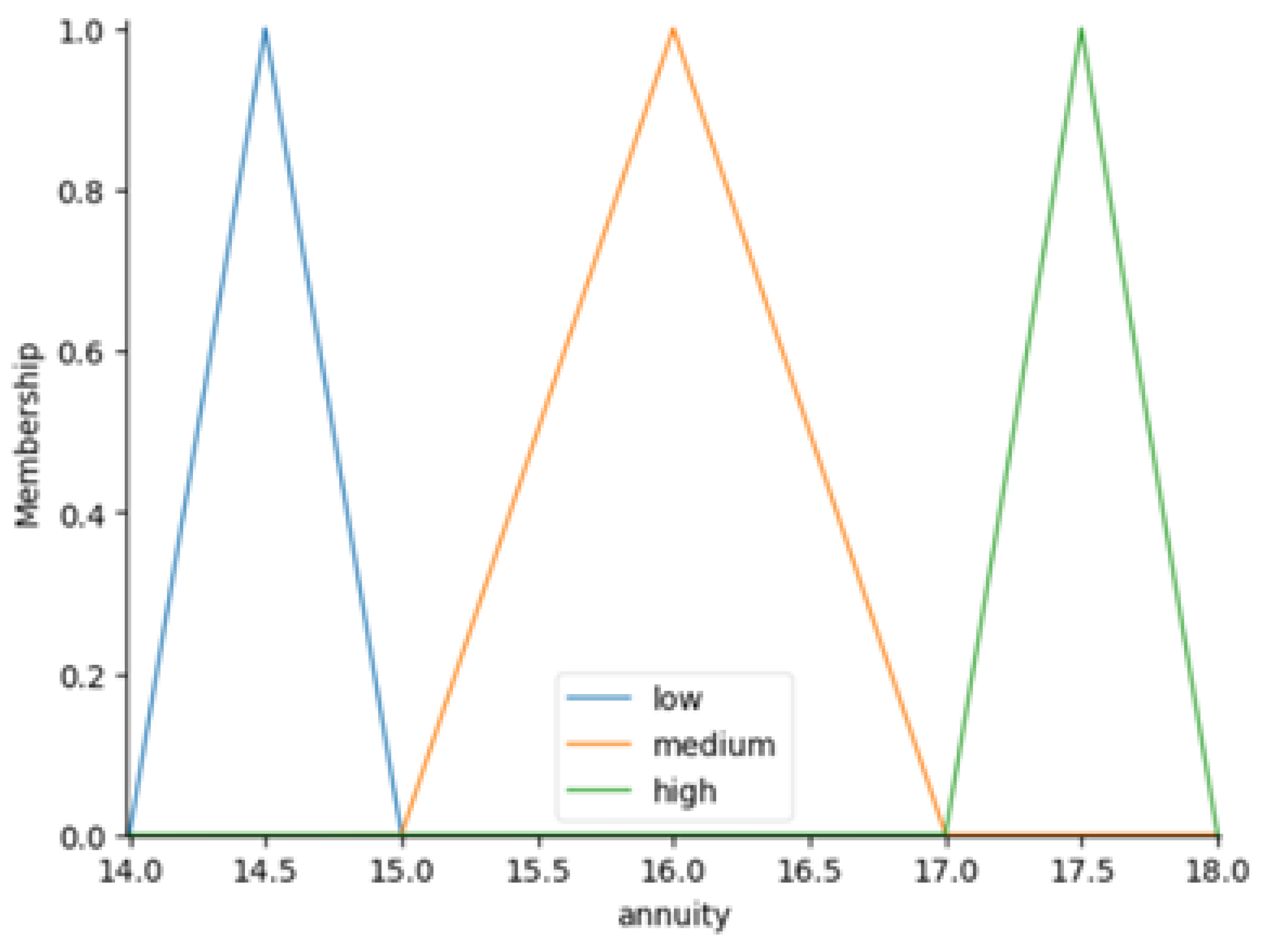
Membership functions are then created for each variable, employing triangular shapes to represent different categories. For example, the annuity variable is divided into the categories “low”, “medium”, and “high”, with centers at 14.0, 15.5, and 17.0, respectively. Additional triangular membership functions are developed for the return rate and contribution rate, with linguistic terms tailored to reflect the unique characteristics of each variable’s range.
The output variable, which is the replacement rate, is also assigned membership functions that describe varying levels of desirability across its possible values. Categories such as “low”, “low to medium”, “medium”, “medium to high”, and “high” are used, covering a range from 0 to 100. Each category is represented by a triangular fuzzy set to indicate degrees of membership. For instance, “low” might correspond to replacement rates under 30.0, “medium” could represent rates between 30.0 and 60.0, and “high” might include rates above 60.0.
Once the membership functions are defined, a series of fuzzy rules is established to determine how the input variables influence the replacement rate. These rules reflect domain-specific knowledge and expert’s insights. For example, one rule might state, “If the annuity is high, the return rate is low, and the contribution rate is medium, then the replacement rate is medium to high”, producing consistent and meaningful output for a specific combination of input values.
| Algorithm 3 Mamdani Fuzzy Inference System (FIS) |
- 1:
Define Universe Variables and Membership Functions - 2:
Define antecedent variables (e.g., , , ) and consequent variable (Y) with linguistic terms (e.g., low, medium, high) - 3:
Define membership functions for each antecedent variable using triangular or Gaussian functions - 4:
Define membership functions for the consequent variable with linguistic terms and corresponding fuzzy sets - 5:
Define Fuzzy Rules - 6:
Define a set of fuzzy rules linking antecedent variables to consequent variables: - 7:
- Rule 1: If is low and is high, then Y is medium - 8:
- Rule 2: If is medium and is low, then Y is high - 9:
- … - 10:
Create Fuzzy Control System - 11:
Create a fuzzy control system using the defined rules - 12:
Initialize the fuzzy control system simulation - 13:
Apply Inputs and Compute Outputs - 14:
for each input set in the dataset do - 15:
Pass input values to the fuzzy control system simulation - 16:
Compute the inferred output using the fuzzy inference mechanism - 17:
Store computed fuzzy output in the dataset - 18:
end for
|
Finally, a control system is built to facilitate the inference process. This system integrates all the defined rules and membership functions, creating a comprehensive framework for decision-making based on fuzzy logic principles. These principles allow for the simulation of the control system with specific input values. That is, when inputs are processed through the FIS, the system generates outputs designed to be straightforward and easy to understand.
3.6. Conceptual Integration Framework Through Analytic Hierarchy Process
To establish a unified and interpretable decision-support framework, this subsection formalizes the conceptual integration of the DL and Mamdani FIS results using the AHP [
31]. The AHP provides a multi-criteria decision-making structure in which each modeling paradigm is evaluated under several criteria reflecting quantitative performance and qualitative interpretability.
3.6.1. Definition of Alternatives and Criteria
Let the set of modeling alternatives be:
and let the evaluation criteria be:
Each alternative
is evaluated under each criterion
by means of a normalized score
, forming the performance matrix:
3.6.2. Criterion-Specific Score Computation
For each criterion
, a raw metric
is computed from the output of model
. To enable comparison across heterogeneous scales, the normalized score is defined as:
where
Specifically:
Accuracy (
): quantified by the MAE, denoted
; its explicit formula is given in
Appendix A. Since smaller values indicate better accuracy, the undesirable form in Equation (
16) applies.
Interpretability (
): represented by
where
denotes the number of fuzzy rules (FIS) or neurons per layer (DL),
is the fuzzy entropy of the rule base, and
is a sparsity or feature-importance index from SHAP values.
Stability (
): quantified by the variance
of model predictions under small input perturbations; the corresponding measure is
with larger values denoting more stable behavior.
Computational Cost (
): expressed by the total training time
or parameter count
,
for which the undesirable form of Equation (
16) applies.
3.6.3. AHP Weight Determination
In the AHP, pairwise comparisons between criteria define the positive reciprocal matrix:
The criterion weights
are obtained as the normalized principal right eigenvector of
:
Consistency of judgments is assessed via the consistency ratio (CR),
where RI is the random index for a matrix of order
m (given by Saaty [
31]);
indicates satisfactory consistency.
3.6.4. Integration of FIS-Derived Fuzzy Weights
The FIS yields fuzzy weights
representing the subjective importance of each criterion
. Each fuzzy weight is characterized by its membership function
, with
(see
Appendix B for more details). Defuzzification by the centroid (center-of-gravity) method produces a crisp equivalent:
The resulting values are normalized so that:
These
may directly replace the eigenvector weights in Equation (
22) or serve to generate a consistent comparison matrix via:
3.6.5. Global Score Aggregation
Given the normalized performance matrix
and the criterion weights
(or
), the overall score of each alternative
is:
and the preferred model is selected as
3.6.6. Illustrative Example and Discussion
Table 5 reports a simplified example with hypothetical normalized scores and AHP-derived weights.
In this hypothetical case, the Hybrid model attains the highest global score (), representing the best compromise among the four evaluation criteria.
Equations (
13)–(
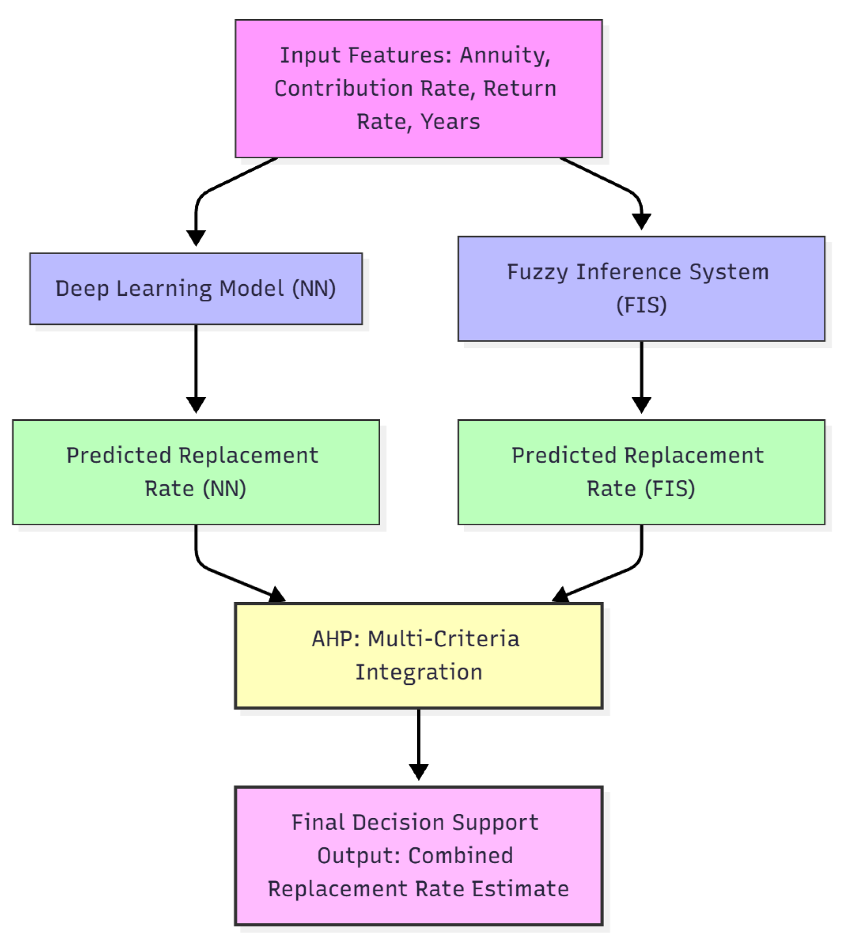
28) formalize how AHP can systematically integrate DL and FIS outputs into a coherent multi-criteria decision-support framework. The DL model contributes quantitative precision (via lower MAE), while the FIS provides qualitative interpretability and fuzzy-derived weighting of criteria. The AHP layer then aggregates these complementary perspectives into an analytically consistent decision metric (see
Figure 2). Although implemented here conceptually, this formulation establishes a rigorous mathematical foundation for future hybrid systems that combine predictive performance and expert reasoning in pension planning.
4. Computational Experiments and Results
4.1. Computer Specifications and Model Implementation Framework
The experiments were conducted on a system featuring an AMD Ryzen 5 5500U processor with Radeon Graphics, operating at a base speed of 2.10 GHz. The computer was equipped with 8 GB of RAM, with about 5.83 GB available for use, and ran on the 64-bit version of Windows 11 Pro. Python served as the primary programming language for implementing the study’s methodologies.
The deep learning models were implemented using the Keras Sequential API, which allows a clear and structured definition of neural network architectures as sequences of layers. In this framework, the model parameters are optimized by minimizing a loss function, which in our case is the mean squared error. The choice of MSE was motivated by its stability during training and its sensitivity to large deviations, making it suitable for financial predictions where significant errors can have high impact. Complementary metrics, including MAE and MAPE, were used during evaluation to provide interpretable insights for decision-makers. These metrics, together with the formal definitions of network transformations and loss functions, are detailed in
Section 3.2 of the methodology, as well as in
Appendix A.
4.2. Data Preparation
We generated a synthetic dataset consisting of 500,000 entries, each capturing three key financial parameters: annuity, return rate, and contribution rate. The annuity values ranged from 14.00 to 18.00, with an average close to 16.00 and a standard deviation of 1.15, indicating a moderate degree of variation. The return rate spanned from 2.00 to 6.00, averaging around 4.00 with a comparable standard deviation. Contribution rates showed an average of approximately 8.00, fluctuating between 6.00 and 10.00, also with a standard deviation of 1.15.
The dataset was partitioned into training (80%) and test (20%) subsets, with the training subset further used in a five-fold cross-validation scheme for model selection and hyperparameter optimization.
4.3. Baseline Neural Network Approach Results
In our baseline neural network, we used the Keras Sequential API to build a straightforward layered architecture [
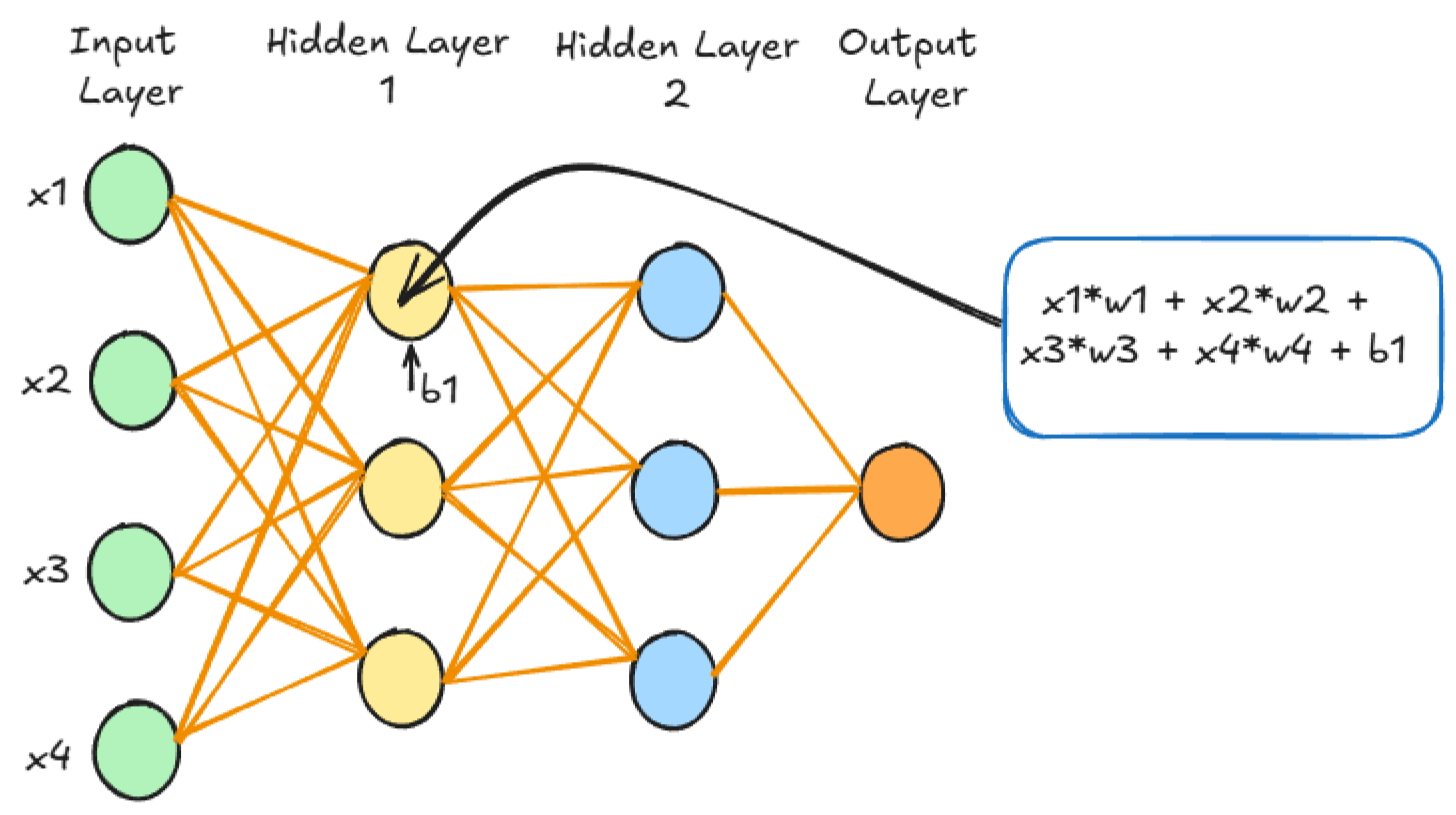
32]. The network included an input layer, three hidden layers, and an output layer. The input layer matched the number of features in the dataset, while the hidden layers had 64, 32, and 16 neurons, respectively, with ReLU as the activation function (ReLU was chosen because it introduces non-linearity into the model, enabling it to effectively learn and represent complex patterns in the data).
To prevent overfitting, we added dropout layers after each hidden layer with a 20% dropout rate (this regularization technique temporarily deactivates a random subset of neurons during training, encouraging the model to rely on a broader set of features and improving its ability to generalize to unseen data). The output layer used a single neuron with a Softplus activation function, ensuring non-negative predictions, which are important for regression tasks.
The model was trained on the dataset over 100 epochs (each epoch represents one complete pass through the entire dataset) with a batch size of 32, allowing the data to be processed in manageable chunks before updating the model’s weights (this setup struck a balance between computational efficiency and stable training dynamics). To guide the optimization process, we used the MSE loss function to measure prediction accuracy and the Adam optimizer with a learning rate of 0.001 to fine-tune the weights efficiently (Adam optimizer adjusts the learning rate during training, ensuring efficient convergence while minimizing the loss function).
When tested on the evaluation dataset, the model achieved an MAE of approximately 1.086. This metric, which reflects the average magnitude of prediction errors, indicated that the model’s predictions were closely aligned with the actual values (a lower MAE suggests strong predictive accuracy, confirming the network’s capability in addressing this regression task).
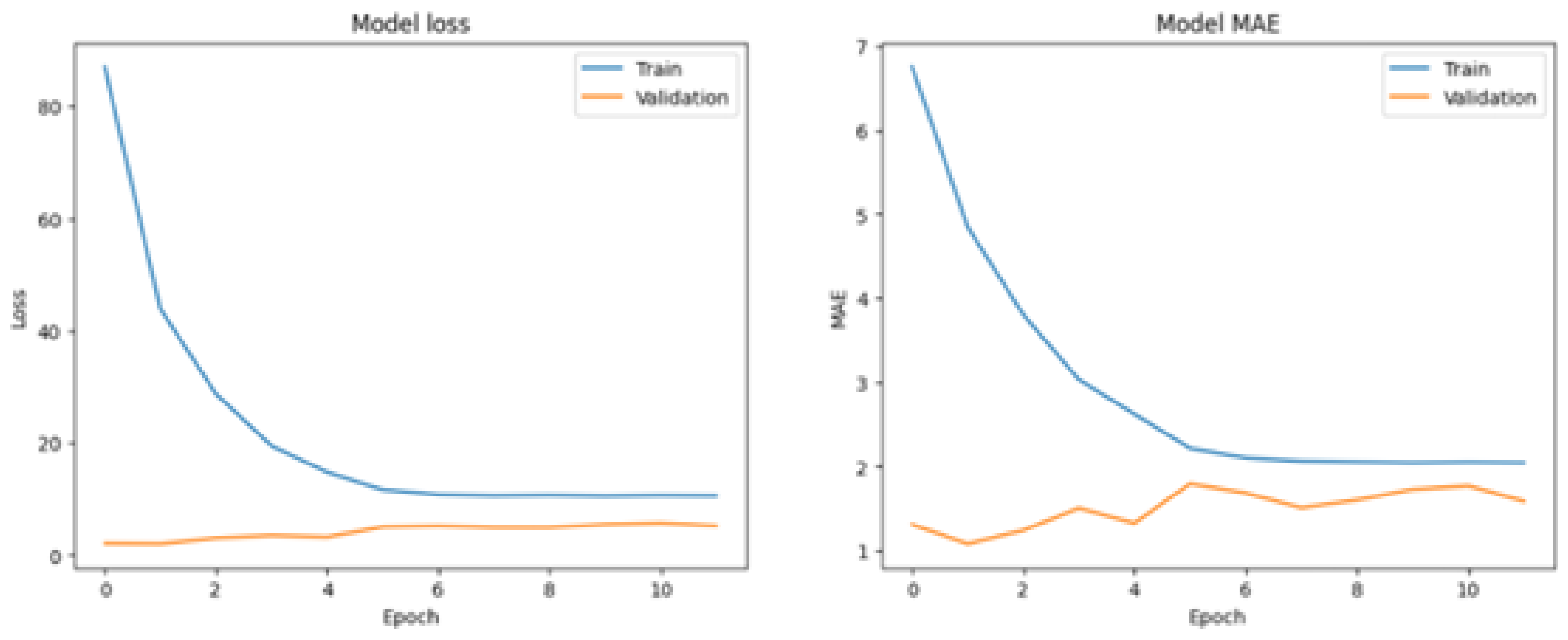
To further evaluate the baseline model’s performance and identify areas for improvement, we generated a series of diagnostic visualizations. One key plot, shown in
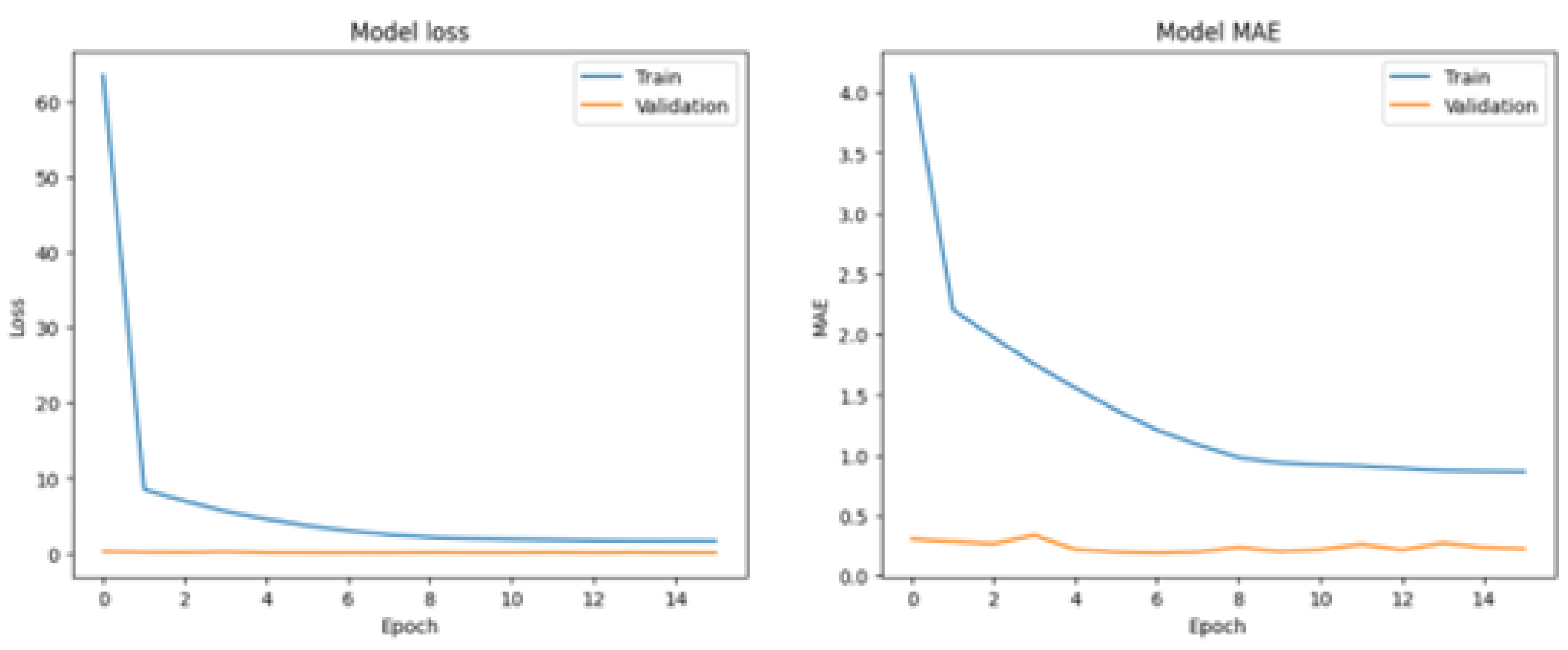
Figure 3, illustrates the loss and MAE trends across training epochs for both the training and validation datasets. This visualization is invaluable for understanding the model’s learning progression. Ideally, it demonstrates a steady decline in both loss and MAE, indicating that the model is improving without signs of overfitting.
The second visualization (
Figure 4) presents a line plot of residuals, offering a detailed look at the model’s predictive errors. Residuals are the differences between the predicted values and the actual target values. In this plot, the residuals fluctuate, revealing that while the model performs well overall, there are instances where its predictions deviate significantly from the actual outcomes. These deviations suggest room for improvement, emphasizing the need for additional model refinement and optimization to minimize fluctuations and boost overall accuracy.
The third visualization (
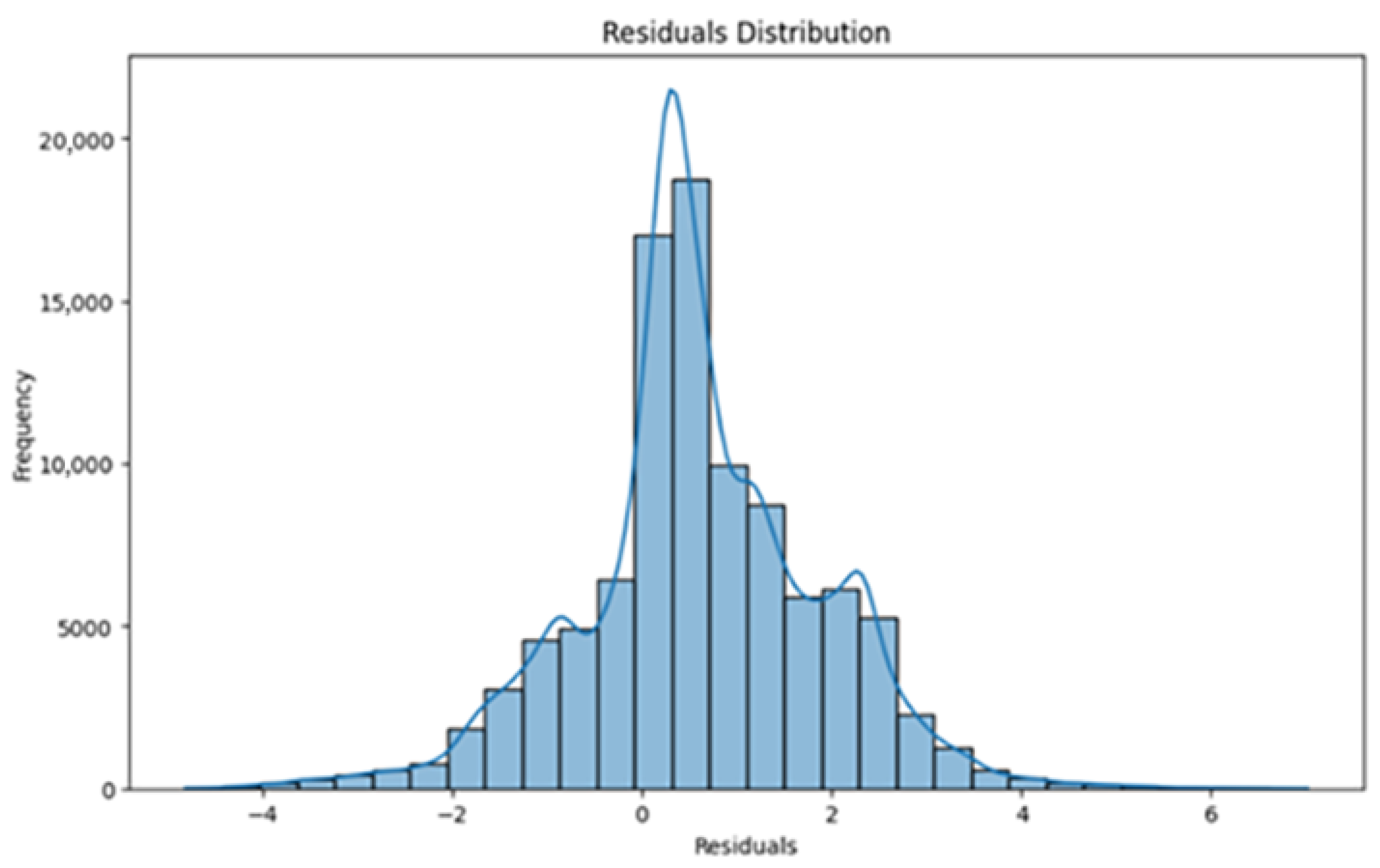
Figure 5) illustrates the distribution of residuals using a histogram, providing a clear overview of the prediction errors across the dataset. Most residuals are concentrated between −2 and 2, indicating that the model’s predictions are generally close to the actual values. However, there are some noticeable outliers, particularly at the distribution’s tails, where residuals range from −4 to −2 and from 4 to 6. These outliers highlight cases where the model’s predictions differ significantly from the true values, pointing to areas where adjustments to the model or input features could improve performance.
Together, these visualizations offer a comprehensive evaluation of the baseline neural network model’s performance. They highlight the model’s ability to learn from the data and produce accurate predictions while also pinpointing areas that could benefit from further fine-tuning. By analyzing these insights, we can make targeted improvements to the model, enhancing its effectiveness in the regression task.
4.4. Optimized Neural Network Approach
To improve the predictive accuracy of the neural network model, we systematically tested several configurations and carefully documented their results. The first setup, with a single hidden layer of 64 neurons, achieved a notably low MAE of 0.2006. Building on this, we explored a second configuration with two hidden layers (64 and 32 neurons), which resulted in a slightly higher MAE of 0.3472. Adding a third hidden layer (64, 32, and 16 neurons) increased the MAE to 0.6720, indicating that greater complexity did not necessarily improve performance.
When we expanded to four hidden layers (64, 32, 16, and 8 neurons), the MAE rose further to 1.2302. Finally, a configuration with five hidden layers (64, 32, 16, 8, and 4 neurons) recorded the highest MAE of 1.9828, suggesting diminishing returns with increased depth. Interestingly, the model with the lowest MAE (0.2006) also demonstrated strong overall performance across additional metrics, providing a balanced and effective solution. These included MSE (to measure the average squared differences between predicted and actual values, serving as an indicator of prediction variance), RMSE (to offer a more intuitive interpretation by aligning its scale with the target variable’s units), (to assess how much of the variation in the target variable can be explained by the predictors, with values close to 1 reflecting a better fit), (to account for the number of predictors, providing a refined measure of model fit, particularly for complex models), and MAPE (to express prediction errors as a percentage of the actual values, offering a practical perspective on the relative magnitude of errors).
In all our experiments, we kept parameters like the number of epochs, batch size, activation functions, and optimization methods consistent with those used in the baseline neural network configuration. This allowed us to directly compare performance differences and attribute them to changes in the network’s architecture. With this approach, we could carefully assess the impact of model complexity on predictive accuracy, finding a balance between simplicity and complexity that worked best for our objectives.
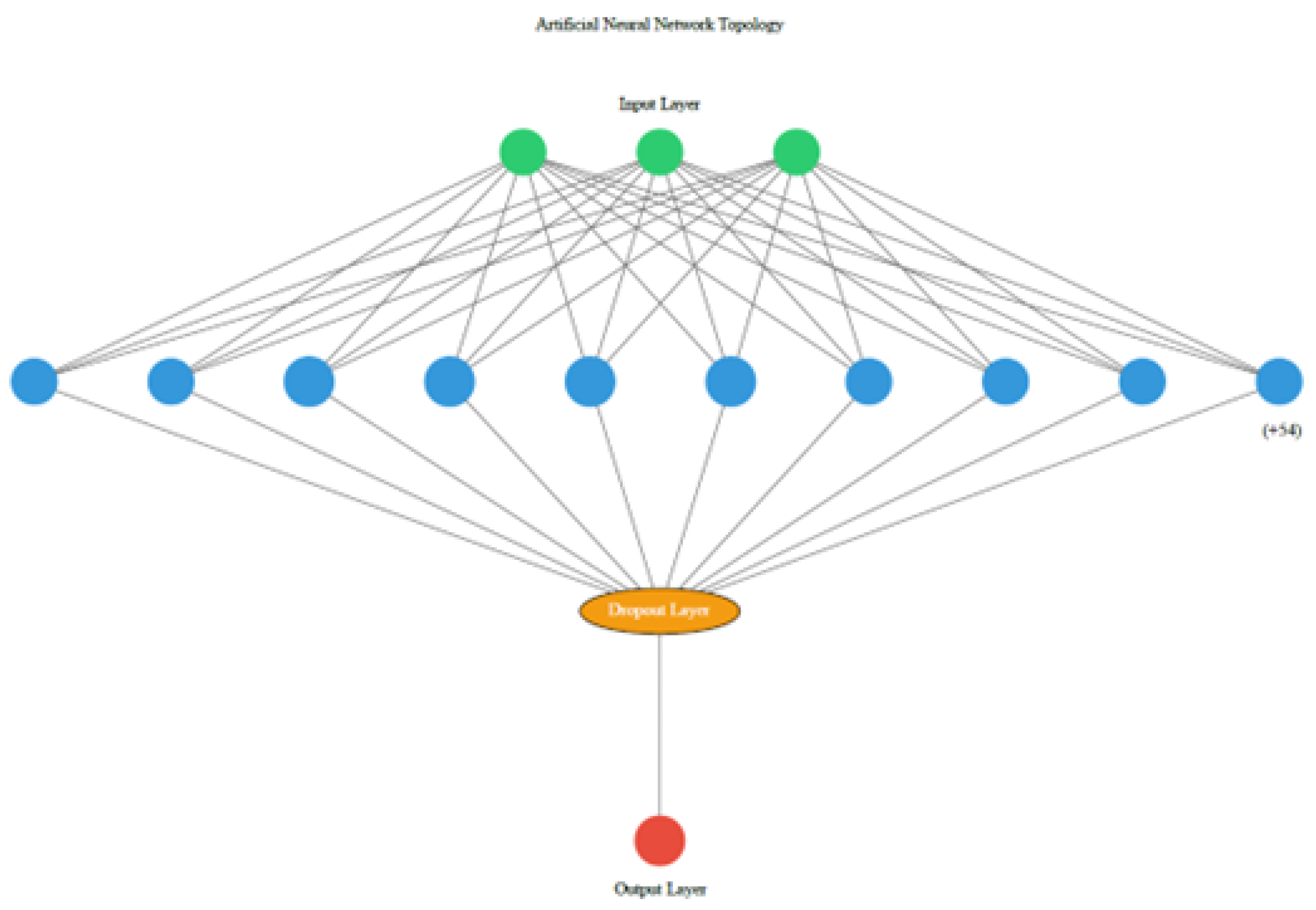
The configuration that performed best consisted of a single hidden layer with 64 neurons (
Figure 6), achieving an MAE of 0.2006. But the numbers tell only part of the story. The model’s performance was further highlighted by its impressively low error values, including an MSE of 0.0718, RMSE of 0.2680,
of 0.9995, and an
of 0.9995. What stood out most, however, was its minimal MAPE of 0.0055, which underscores the model’s reliability in delivering accurate predictions. This not only confirms the model’s effectiveness but also makes it a robust solution for the regression task.
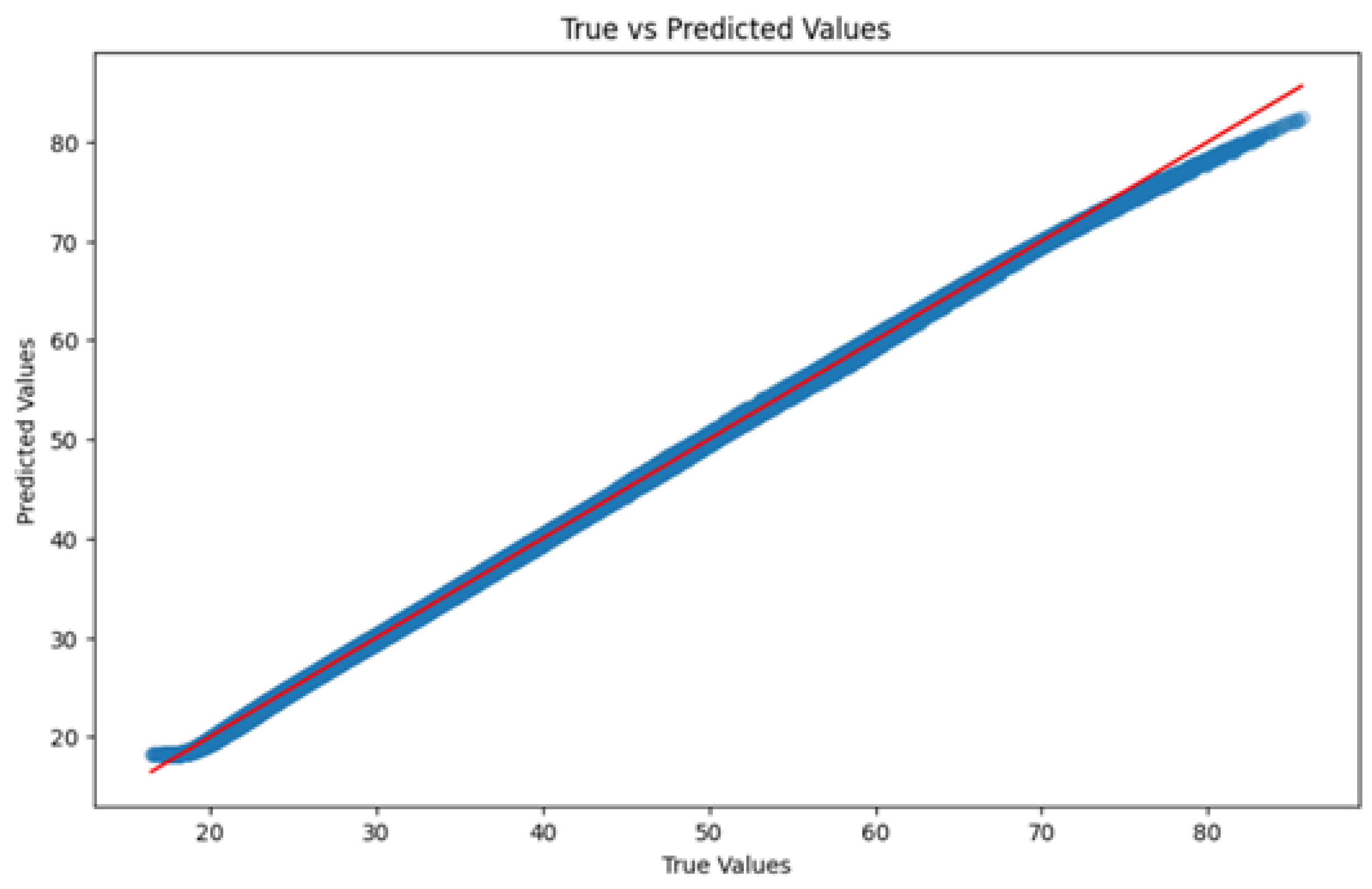
In contrast to the baseline model, the optimized neural network configurations have shown notable improvements in model performance metrics. The line plot (
Figure 7 and
Figure 8) depicting the convergence of model loss and MAE over epochs indicates enhanced stability and faster convergence during both training and validation phases.
Furthermore, the distribution plot of residuals (
Figure 9) reveals a significant refinement. Most residuals are now concentrated within a narrower range, specifically between −1 and 1, indicating that the model predictions align closely with the actual values for most instances. There are some outliers visible on the right tail extending up to 3, but their reduced frequency compared to the baseline suggests better overall model accuracy and consistency.
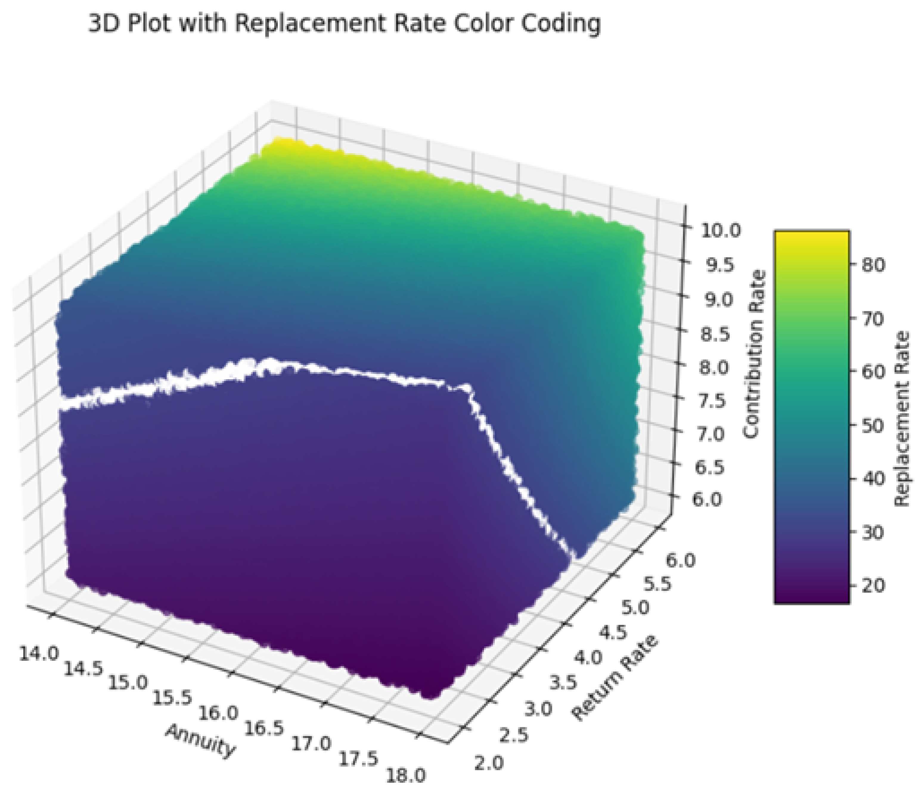
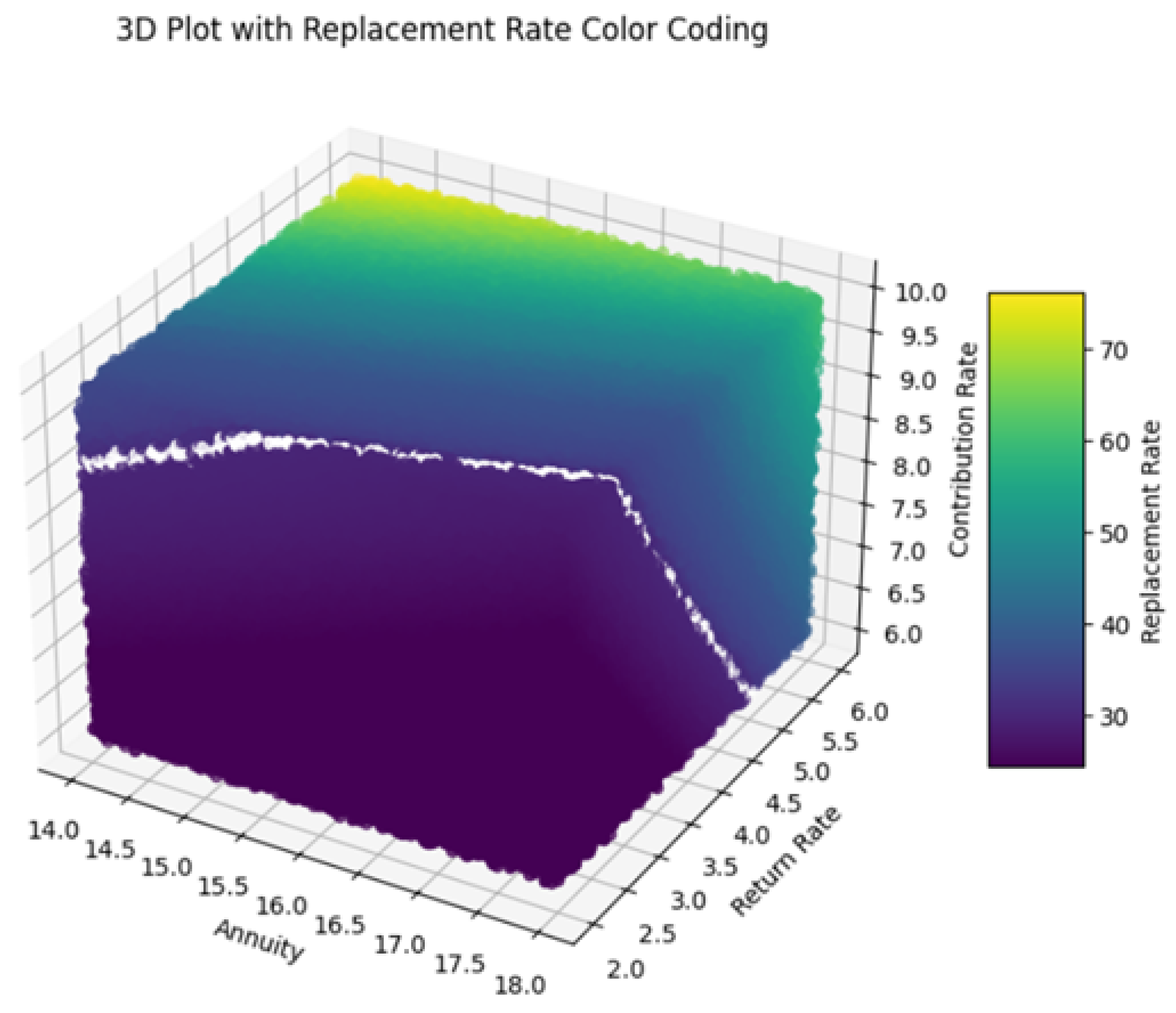
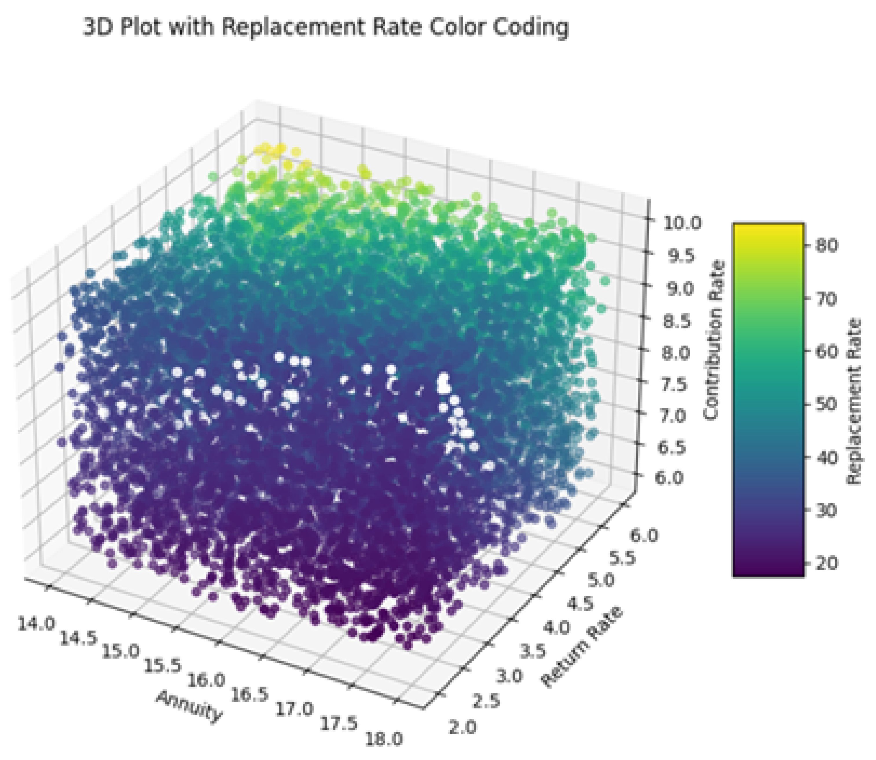
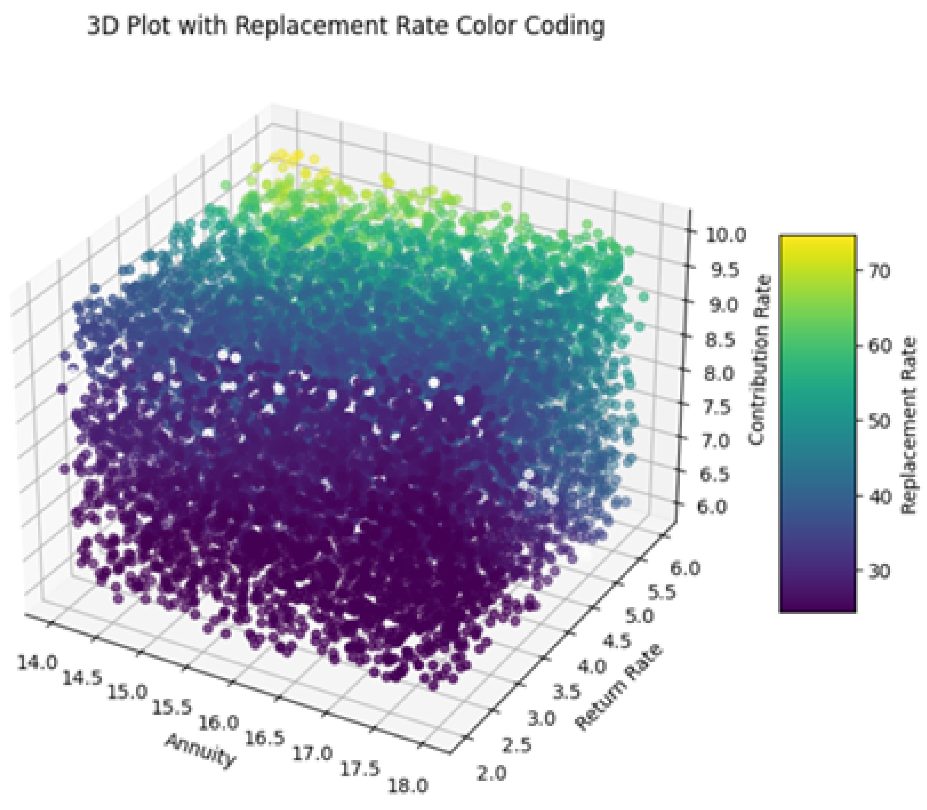
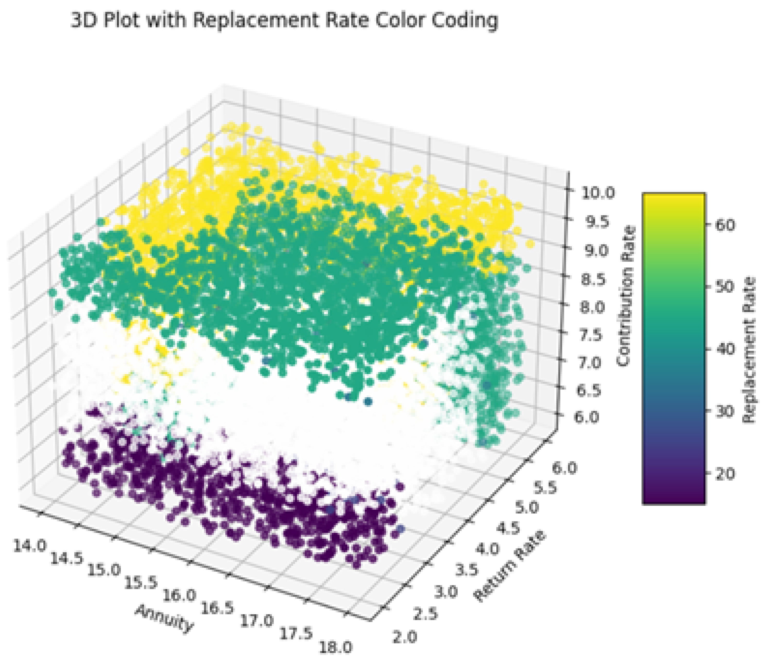
In addition to this, the following 3D plots (
Figure 10 and
Figure 11) visualize the relationship between the variables annuity, return rate, and contribution rate, with the color of each data point representing the corresponding actual replacement rate (computed with exact formulas mentioned in previous sections) and replacement rate predicted by the optimized neural network model. Each axis of the plot represents a different variable: annuity, return rate, and contribution rate. The color bar on the right side of the plot indicates the scale of replacement rates, ranging from lower values (purple) to higher values (yellow).
The plot reveals how different combinations of annuity, return rate, and contribution rate contribute to actual (
Figure 10) and predicting replacement rates (
Figure 11). Data points are scattered across the plot, with colors varying based on the replacement rate values. The colormap helps distinguish between different levels of replacement rates, facilitating visual interpretation of the predictions.
The use of color coding plays a key role in enhancing the interpretability of the model’s performance across the dataset. In particular, we are visually distinguishing areas where the model accurately predicts replacement rates (shown by consistent color regions) from those where discrepancies or outliers exist (indicated by shifts in color). This approach provides an intuitive way to assess prediction quality. The inclusion of white as a marker for replacement rates around 30 further aids clarity, effectively highlighting specific ranges of both actual values and predictions.
In both visualizations, the data points are carefully color-coded to represent predicted replacement rates, with white explicitly indicating values close to 30. The presence of consistently white-colored data points suggests that the models perform exceptionally well when predicting replacement rates near this threshold. This uniformity reflects the accuracy of the models and indicates their ability to handle scenarios around this key value with minimal error. The similarity observed between the two visualizations reinforces the models’ effectiveness in generalizing across the dataset, capturing the relationships between input variables and replacement rates with remarkable consistency.
These results (see
Table 6) underscore the reliability and precision of the neural network models in estimating replacement rates. By successfully learning the underlying patterns in the data and delivering stable predictions, the models demonstrate their capability to achieve high levels of accuracy in this regression task.
4.5. Mamdani Fuzzy Inference System
The Mamdani FIS designed for predicting replacement rates utilizes linguistic variables defined over specific intervals for its inputs and outputs. Here are the linguistic variables and their intervals:
Inputs:
- −
Annuity: Low [13.99–15.0], Medium [14.0–17.0], High [17.0–18.01];
- −
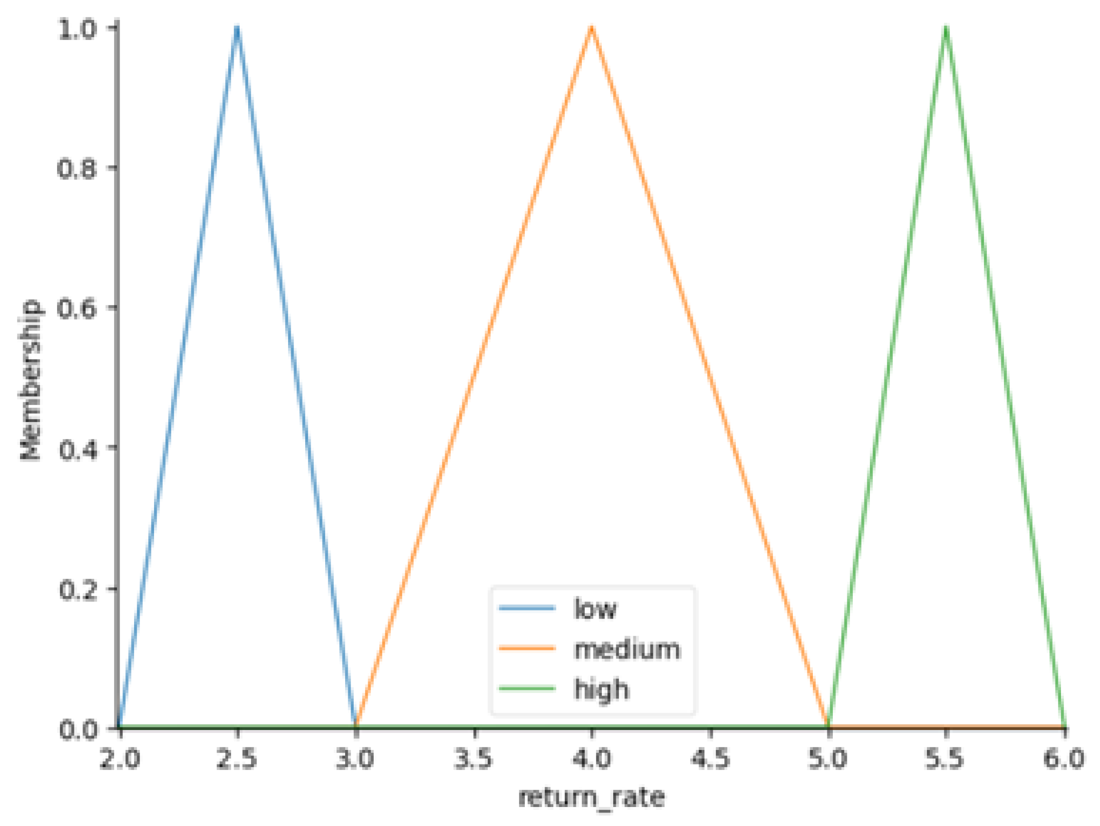
Return Rate: Low [1.99–3.0], Medium [2.0–5.0], High [5.0–6.01];
- −
Contribution Rate: Low [5.99–7.0], Medium [6.0–9.0], High [9.0–10.01].
Output:
- −
Replacement Rate: Low [0.0–30.0], Low to Medium [0.0–60.0], Medium [30.0–100.0], Medium to High [30.0–100.0], High [60.0–100.0].
The Mamdani FIS employs 27 fuzzy rules to map the input variables to the output replacement rate. These rules are defined as follows:
If annuity is low and return rate is low and contribution rate is low, then replacement rate is low.
If annuity is low and return rate is medium and contribution rate is low, then replacement rate is medium.
If annuity is low and return rate is high and contribution rate is low, then replacement rate is medium to high.
If annuity is low and return rate is low and contribution rate is medium, then replacement rate is low to medium.
If annuity is low and return rate is medium and contribution rate is medium, then replacement rate is medium to high.
If annuity is low and return rate is high and contribution rate is medium, then replacement rate is medium to high.
If annuity is low and return rate is low and contribution rate is high, then replacement rate is medium.
If annuity is low and return rate is medium and contribution rate is high, then replacement rate is medium to high.
If annuity is low and return rate is high and contribution rate is high, then replacement rate is medium to high.
If annuity is medium and return rate is low and contribution rate is low, then replacement rate is low.
If annuity is medium and return rate is medium and contribution rate is low, then replacement rate is low to medium.
If annuity is medium and return rate is high and contribution rate is low, then replacement rate is medium to high.
If annuity is medium and return rate is low and contribution rate is medium, then replacement rate is low to medium.
If annuity is medium and return rate is medium and contribution rate is medium, then replacement rate is low to medium.
If annuity is medium and return rate is high and contribution rate is medium, then replacement rate is medium to high.
If annuity is medium and return rate is low and contribution rate is high, then replacement rate is medium.
If annuity is medium and return rate is medium and contribution rate is high, then replacement rate is medium.
If annuity is medium and return rate is high and contribution rate is high, then replacement rate is medium to high.
If annuity is high and return rate is low and contribution rate is low, then replacement rate is low.
If annuity is high and return rate is medium and contribution rate is low, then replacement rate is low to medium.
If annuity is high and return rate is high and contribution rate is low, then replacement rate is medium.
If annuity is high and return rate is low and contribution rate is medium, then replacement rate is low to medium.
If annuity is high and return rate is medium and contribution rate is medium, then replacement rate is low to medium.
If annuity is high and return rate is high and contribution rate is medium, then replacement rate is medium.
If annuity is high and return rate is low and contribution rate is high, then replacement rate is medium.
If annuity is high and return rate is medium and contribution rate is high, then replacement rate is medium.
If annuity is high and return rate is high and contribution rate is high, then replacement rate is medium to high.
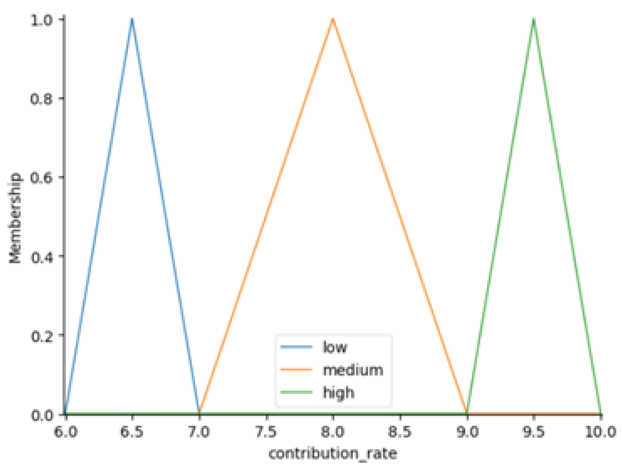
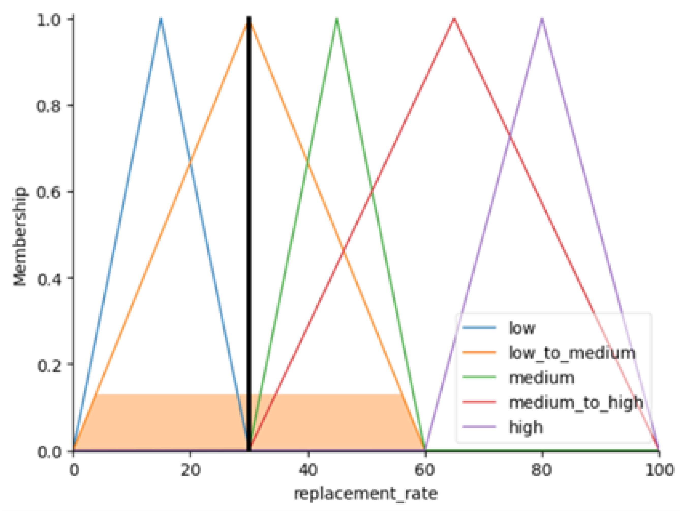
Figure 12,
Figure 13,
Figure 14 and
Figure 15 depict the triangular membership functions for the input variables of interest (i.e., annuity, return rate and contribution rate), as well as the output variable of interest (i.e., replacement rate).
As an illustrative example, consider the following values:
Annuity: 16.746141;
Return rate: 3.67;
Contribution rate: 7.13.
Using the membership degrees, the Mamdani FIS applies the rules and aggregates them using triangular membership functions for the output replacement rate. In this case, it predicts a replacement rate of approximately 30.0, demonstrating how the Fuzzy Inference System effectively handles inputs and generates corresponding outputs based on fuzzy logic principles (
Figure 16).
In order to mitigate computational demands, the Mamdani FIS was applied to a subset of 11,000 samples from the dataset. Similar to our previous analysis, 3D plots were generated to compare the behavior of the FIS-predicted replacement rate values against those predicted by the optimized neural network (
Figure 17). Upon examination, it was observed that the neural network’s predicted values closely approximated the actual replacement rates (
Figure 18). However, contrasting results were noted with the FIS predictions (
Figure 19), revealing significant fluctuations. This suggests that further investigation is necessary to refine the rules and membership function intervals according to expert knowledge and preferences.
Investing more time and effort into refining these aspects is crucial for achieving a closer alignment between the FIS (i.e., the predictive accuracy and stability of the FIS) and the desired outcomes (i.e., estimated replacement rates). While the FIS method offers valuable advantages, especially in dealing with uncertain or imprecise data through fuzzy logic, it also comes with its own set of challenges. One key obstacle is the heavy reliance on expert knowledge to design rules and membership functions. If these rules are not clearly defined, the predictions may become unreliable, leading to inconsistent outcomes. This highlights the critical role experts play in optimizing FIS models and ensuring their effectiveness. Ultimately, developing precise rules and carefully tuning the parameters are essential steps for making the most of the FIS approach.
4.6. Discussion and Practical Considerations
4.6.1. Data Quality and Availability for Neural Networks
Implementing neural networks in real-world pension fund scenarios entails several challenges related to data quality and availability. Pension datasets are often incomplete or contain noisy entries due to reporting errors or heterogeneous data sources. Our synthetic experiments (see
Table 6 and
Figure 8,
Figure 9,
Figure 10 and
Figure 11) demonstrate that the optimized neural network can achieve high predictive accuracy (MAE = 0.2006,
) under controlled conditions. In practice, preprocessing techniques such as imputation, outlier removal, and normalization, along with data augmentation strategies, can help mitigate the impact of missing or noisy data, ensuring robust model performance.
4.6.2. Dynamic Updating of Fuzzy Rules
The Mamdani Fuzzy Inference System relies on expert-defined rules and membership functions, which may need frequent updates in response to fluctuating macroeconomic conditions, such as changes in interest rates, inflation, or pension policy. While our experiments applied the FIS to a subset of 11,000 samples (
Figure 17,
Figure 18 and
Figure 19), demonstrating reasonable performance, practical implementation would require a dynamic rule adaptation mechanism. Techniques such as adaptive fuzzy systems, rule-weight adjustment, or integration with reinforcement learning could allow the FIS to automatically adjust its rules over time, maintaining predictive accuracy in changing environments.
4.6.3. Interpretability of Neural Networks
One limitation often associated with deep learning models is their ‘black-box’ nature. In the context of pension advisory services, transparency and interpretability are critical for client trust and regulatory compliance. Our 3D visualizations (
Figure 10 and
Figure 11) help interpret the relationship between input parameters and replacement rates, but additional methods such as SHAP (SHapley Additive exPlanations) or LIME (Local Interpretable Model-agnostic Explanations) can further elucidate feature contributions [
33,
34]. These tools can provide insight into individual predictions, supporting explainable and accountable AI deployment in financial decision-making.
4.6.4. Cost-Effectiveness Compared to Traditional Methods
The development, deployment, and maintenance of AI-based systems involve initial investment and technical expertise. However, once implemented, neural networks and FIS models can process large-scale pension datasets with minimal human intervention, offering scalability and operational efficiency. For small and medium-sized pension funds, this automation may reduce reliance on highly specialized financial experts, streamline estimation of replacement rates, and enable rapid scenario analysis. Our results indicate that AI models can achieve precise and consistent predictions (e.g., neural network MAE = 0.2006), suggesting potential advantages in both accuracy and cost-effectiveness over traditional approaches while maintaining the ability to integrate expert knowledge where necessary.
4.6.5. Integration Through AHP and Hybrid Evaluation
Beyond the individual analysis of the DL and Mamdani FIS models,
Section 3.6 introduced a conceptual framework based on the AHP to integrate both approaches within a unified decision-support structure. This framework enables a balanced evaluation of the models by considering multiple criteria such as predictive accuracy, interpretability, stability, and computational cost in a structured, transparent way.
Under this scheme, the DL and FIS models are treated as decision alternatives, while their respective performance metrics provide the criterion scores. The AHP weighting mechanism, optionally enhanced by fuzzy-derived importance factors from the FIS, allows decision-makers to compute a composite score reflecting the overall desirability of each modeling approach. Conceptually, this hybrid evaluation layer demonstrates how quantitative precision from DL can be systematically combined with the qualitative interpretability of FIS to support informed, multi-criteria pension planning decisions.
Although this integration is introduced conceptually rather than implemented empirically in the present study, it strengthens the methodological coherence between the two computational paradigms and outlines a concrete pathway for future work on hybrid AI-based decision-support systems in the pension domain.
5. Conclusions and Future Remarks
This research set out to find better ways to estimate replacement rates, which are key to planning for retirement. We focused on two main approaches: neural networks and the Mamdani FIS. The neural networks showed great promise, with low MAE and steady progress during training. On the other hand, the FIS method proved especially useful when dealing with the uncertainties that often arise in retirement planning. It became clear that the effectiveness of the FIS approach relies heavily on well-defined rules from experts and careful parameter adjustments.
Several limitations of the current study should be acknowledged. First, the analysis relied on synthetic data to enable controlled benchmarking, which limits the immediate applicability of the models to real-world pension systems. Second, the FIS approach, while interpretable, requires expert knowledge for rule definition, which may not always be readily available. Third, the neural network, although accurate, can be less interpretable and may require extensive hyperparameter tuning for optimal performance. Finally, the study considered a relatively small set of input variables, leaving room for expanding the feature space to capture additional financial or demographic factors.
This study also proposed a conceptual integration framework combining neural network and FIS outputs through the AHP, which enables systematic weighting of criteria such as prediction accuracy, interpretability, and stability in pension planning decisions. Future research should focus on the empirical implementation of this hybrid framework using real-world pension datasets, exploring larger and more diverse feature sets, and assessing its robustness in practical settings. Additional enhancements could include the incorporation of explainability tools for neural networks, such as SHAP or LIME, to improve transparency and trust, and further refinement of FIS rules to enhance interpretability and stability.
In addition, the AHP can provide valuable insights and enhance the robustness of the decision-making process. Specifically, AHP facilitates systematic comparisons of pension strategies by evaluating multiple criteria within a hierarchical framework (see
Figure 20). For instance, when assessing and selecting pension strategies (i.e., alternatives), decision-makers can prioritize criteria such as prediction accuracy, risk management, and alignment with broader financial objectives. This approach enables a more effective evaluation of alternatives and supports informed decision-making tailored to individual requirements. Moreover, both individual and group decision-making processes can benefit from the AHP methodology, promoting consistency and agreement in decisions.
In conclusion, this study highlights the efficacy of neural networks in estimating replacement rates and underscores the potential of FIS models, provided that they undergo further refinement. Moreover, the integration of these approaches through the AHP offers a structured, multi-criteria decision-support framework that leverages the complementary strengths of both methods. Future advancements in retirement planning methodologies can help individuals and financial advisors make better-informed choices and achieve more reliable outcomes.
