Abstract
Alzheimer’s disease (AD) affects over 55 million individuals worldwide, yet no transformative disease-modifying therapies exist. Mathematical modelling provides a powerful framework to elucidate complex disease mechanisms, predict therapeutic outcomes, and enable precision medicine—capabilities urgently needed where multiscale spatiotemporal processes defy experimental analysis alone. We developed a mechanistic spatiotemporal model coupling four AD hallmarks: β-amyloid (Aβ) accumulation, T-protein (T-p) aggregation, neuroinflammation and electrical conductivity decline. Formulated as non-linear partial differential equations (p.d.es) on a 3-dimensional biological interpretation of non-linear terms (the ellipsoidal brain domain with biologically grounded parameters), the model was solved using eigenfunction expansion, Fourier analysis and numerical methods. Therapeutic interventions were simulated through mechanistically motivated parameter modifications and validated against longitudinal biomarker data from major cohort studies. Simulations reveal Aβ-initiated spatiotemporal cascades originating in the hippocampus and spreading radially at 0.15–0.20 cm/year, with T-pathology emerging after 2–3 years. Conductivity decline accelerates upon T-onset (year 5–7), reflecting the transition to symptomatic disease. Multimodal intervention at early symptomatic stages reduces peak Aβ by 36% and inflammation by 52% and preserves 41% more conductivity than untreated controls. Sensitivity analysis identifies Aβ production and inflammatory regulation as critical therapeutic targets, with dose–response curves demonstrating linear efficacy relationships. This biologically grounded framework explicitly links molecular pathology to functional decline, enabling patient-specific trajectory prediction through parameter calibration. The model establishes a foundation for precision medicine applications including individualized prognosis, optimal treatment timing and virtual clinical trial design, advancing quantitative systems biology of neurodegeneration.
MSC:
92-10
1. Introduction
Recent years have seen a rapid development of mathematical models for AD and other neurodegenerative disorders, ranging from reaction–diffusion frameworks to network-level transport models, for instance: neural oscillations on evolving networks [1], a multi-physics model of prion-like propagation and tissue atrophy [2], and network-based transport models of T-progression [3,4]. Such multiscale approaches have also been explored in theoretical neuroscience frameworks that couple biophysical diffusion with tissue-level degradation [2]. Building upon these advances, the present study extends previous p.d.e approaches by explicitly coupling electrical conductivity dynamics with molecular pathology, offering a unified quantitative description of AD progression.
AD is a chronic neurodegenerative disorder, characterized by a slow but relentless deterioration of brain structure and function. Comparable multiscale progression has been documented in computational studies integrating molecular and electrophysiological markers [5]. Its core biological features include the accumulation of Aβ deposits, the formation of T-p neurofibrillary tangles, the progressive loss of electrical conductivity in neural tissue, and the activation of chronic inflammation [6,7,8]. Together, these mechanisms form a complex web of interactions that gradually disrupt neural communication and lead to irreversible cognitive decline.
In this study, we construct and analyze an extended mathematical model that captures these coupled processes in both time and space. The model integrates four essential variables: the concentration of Aβ, the concentration of T-p, the inflammatory index, and the electrical conductivity of the brain tissue. Each of these components interacts dynamically with the others, forming a system of non-linear p.d.es describing how pathology evolves within a realistic 3-dimensional brain geometry.
The brain space Β⊂ℝ3 is approximated by an ellipsoidal region:
where a, b and c represent the semi-axes of the ellipsoid. This choice provides a more accurate geometric and topological approximation of the human brain than the standard cubic or spherical assumptions. The boundary (∂B) defines the brain’s outer surface, while the interior domain (B) sets the region where all dependent variables evolve.
The geometry of (B) serves three purposes. First, it defines the physical domain for all field variables. Second, it specifies the boundary surfaces where flux conditions apply. Third, it determines the eigenfunctions of the Laplace operator that govern diffusion. This explicit spatial formulation makes it possible to explore how localized pathological processes—such as amyloid accumulation in the hippocampus—propagate through the surrounding brain tissue.
The system of equations is formulated to ensure physical, biological, and mathematical coherence. Parameters are selected to preserve stability and reflect biologically observed relationships, while the 1-directional decrease in electrical conductivity represents the entropic progression of AD. The use of an ellipsoidal topology allows us to combine analytical and numerical techniques, including separation of spatial variables, eigenfunction expansions of the Laplacian operator, and Fourier transforms.
Beyond serving as a computational framework, this model aims to provide an interpretative tool. It can link mathematical behavior with biological meaning—showing how early molecular imbalances evolve into functional degradation. Finally, its parameters can be adjusted using clinical or imaging data, making the model adaptable for predictive applications and personalized evaluation of disease progression and treatment outcomes.
2. The Role of Aβ
Aβ is a small peptide derived from the proteolytic processing of the amyloid precursor protein (APP), a membrane protein normally expressed in neurons and other cell types. APP can be cleaved through two distinct enzymatic pathways. The first, known as the non-amyloidogenic pathway, results in harmless fragments. The second, the amyloidogenic pathway, involves β- and γ-secretase activity and leads to the production of Aβ. Once released, Aβ tends to aggregate into a variety of forms—monomers, oligomers, and fibrils—with the latter two being particularly toxic to neurons [3,6,9].
As the concentration of Aβ increases, a series of pathological events is triggered. The peptide deposits in the extracellular space, forming amyloid plaques that interfere with neural signaling and promote oxidative stress. Soluble Aβ oligomers have been shown to disrupt synaptic transmission, leading to communication failure between neurons. The resulting oxidative stress causes damage to cell membranes, mitochondria, and even nuclear DNA. Over time, these processes activate apoptotic pathways, causing neural death. Moreover, Aβ stimulates glial cells—especially microglia and astrocytes—initiating a chronic inflammatory state that further amplifies neural injury.
The escalation of Aβ levels is widely associated with the early stages of AD and represents the molecular starting point of disease progression [6]. As pathology advances, Aβ accumulation coexists with other key processes, including the hyperphosphorylation of T-p into neurofibrillary tangles and the widespread loss of neurons driving cortical atrophy [10]. This early amyloid accumulation is consistent with clinical and experimental findings emphasizing Aβ as the primary initiator of neurodegeneration [11,12].
In the present model, Aβ serves as the central pathogenic variable. It is represented by the spatiotemporal function:
which denotes the concentration of Aβ in the brain as a function of space and time within the ellipsoidal region (B). Production is assumed to occur primarily in specific regions—typically near the center of (B), such as the hippocampus—and diffusion extends outward toward the periphery. This spread is influenced by local inflammatory activity and by interactions with T-pathology.
A(x,y,z,t), (x,y,z,t) ∈ B × [0,t0],
Conceptually, Aβ marks the beginning of the pathological cascade in the model. Its behavior follows a chain of linked processes:
Production → accumulation → diffusion → inflammation → conductivity reduction.
Through this sequence, Aβ drives the emergence and spatial expansion of AD pathology within the ellipsoidal brain space. Its distribution and temporal evolution set the pace of the entire disease mechanism, making it the principal agent that connects molecular pathology to large-scale functional decline.
3. The Role of T-p
T-p is a key intracellular molecule that stabilizes microtubules and maintains the structural integrity of neurons. Under normal conditions, it supports axonal transport and contributes to the dynamic organization of the cytoskeleton. In AD, however, Tau undergoes abnormal hyperphosphorylation, leading to the formation of insoluble aggregates known as neurofibrillary tangles [8]. These tangles accumulate within neurons, disrupt intracellular transport, and eventually cause cell death.
In the present model, T-p is described by the spatiotemporal function:
which expresses the concentration of the pathological T-p within the same ellipsoidal domain (B). The evolution of tau follows a delayed response relative to Aβ dynamics, since T-pathology emerges only after sustained exposure to high Aβ levels. Local peaks of T-p concentration tend to appear in regions where Aβ is already abundant, and the geometry of (B) shapes its diffusion, which remains confined within the brain boundaries (∂B).
T(x,y,z,t), (x,y,z,t) ∈ B × [0,t0],
Biologically, T-p acts as a secondary but decisive mediator of neurodegeneration. It translates the extracellular accumulation of Aβ into intracellular toxicity. As the disease advances, T-p spreads from neuron to neuron, contributing to the breakdown of neural architecture and promoting local inflammation.
In the framework of the model, T-p is produced through the influence of Aβ, diffuses within the cerebral space, and induces structural degeneration and inflammation. It is also naturally degraded or removed through immune and enzymatic mechanisms, and serves as an intermediate link between Aβ accumulation and the reduction in electrical conductivity [8].
Thus, T-p represents the stage at which molecular pathology becomes structurally destructive. Its emergence indicates that the system has shifted from early biochemical imbalance to visible neurofibrillary degeneration—a hallmark of the irreversible phase of AD.
4. The Role of Electrical Conductivity
The gradual reduction in brain electrical conductivity, observed in AD, is a multifactorial outcome of structural and biochemical degeneration. Electrical conductivity depends on the integrity of neural membranes, synaptic connections, and the conductive properties of the surrounding extracellular matrix. Computational network models demonstrate similar conductivity decline patterns arising from topological disconnection and synaptic loss [2,5]. As neurodegeneration progresses, this capacity to transmit electrical signals weakens systematically, reflecting the cumulative damage at both cellular and network levels.
Several biological mechanisms account for this decline. The first involves the degeneration of nerve cells, primarily caused by the accumulation of abnormal protein aggregates. Amyloid plaques disrupt extracellular communication, while intracellular neurofibrillary tangles formed by T-hyperphosphorylated distort the cytoskeleton and impede intracellular transport. As neurons die, synaptic density decreases, reducing the number of available pathways for electrical transmission. A second mechanism concerns changes in myelination and axonal structure. Demyelination slows or blocks the propagation of action potentials, while dendritic retraction and shortening limit the complexity and extent of synaptic networks. The third mechanism involves the loss of neural plasticity—the brain’s capacity to reorganize connections—which diminishes its ability to adapt to new stimuli and compensate for damage.
Inflammation also plays a destructive role. Activated microglia release cytotoxic agents and free radicals, which exacerbate oxidative stress and further impair conductivity. At the same time, disturbances in neurotransmission arise, including reduced acetylcholine release and altered ion channel function, both of which interfere with synaptic signaling. Finally, biochemical imbalances in the extracellular fluid, such as changes in ionic composition (Na+, K+ and Ca++), modify the conductive properties of brain tissue.
Increased Aβ concentration contributes directly to conductivity loss through several routes. It alters synaptic architecture, damages neural membranes, and fosters a pro-inflammatory microenvironment. Moreover, Aβ deposition within vascular structures restricts cerebral blood flow and oxygen delivery, further diminishing neural viability. Collectively, these processes produce measurable reductions in electrical conductivity, which can be detected in experimental studies through electroencephalography (EEG) and related brain-imaging modalities that reveal abnormal network activity patterns.
In the mathematical model, conductivity is expressed as the spatiotemporal variable:
representing the ability of brain tissue to transmit electrical signals. Diffusion is not included for this variable. Instead, conductivity evolves locally at each spatial point as a function of the concurrent values of A, T, and I. The process is unidirectional—essentially decreasing—because each pathological component exerts a damaging effect on conductivity [5]. Competing regenerative mechanisms may exist but are not strong enough to reverse the overall downward trend.
C(x,y,z,t), (x,y,z,t) ∈ B × [0,t0],
As time progresses, Aβ levels rise while conductivity declines, with T-pathology and inflammation accelerating the deterioration. The most pronounced drop in conductivity occurs near the center of the ellipsoidal region (B), where Aβ and T-p concentrations peak. In this formulation, conductivity does not influence the other state variables; it is a cumulative result of their pathological interactions:
A(x,y,z,t) → T(x,y,z,t) → I(x,y,z,t) → C(x,y,z,t).
Hence, C(x,y,z,t) serves as a global biomarker of neural function, integrating the combined impact of amyloid accumulation, T-pathology, and inflammation [7]. It represents the functional state of the brain network and provides a direct mathematical measure of the overall cognitive and structural decline associated with AD [4,5].
5. The Role of Inflammation
Inflammation constitutes one of the most complex and paradoxical components in the pathophysiology of AD. While it initially serves a protective purpose—aiming to clear abnormal proteins and cellular debris—it gradually turns into a chronic and self-perpetuating process that accelerates neural damage [7]. The interaction between Aβ, T-p, and the inflammatory response forms a self-reinforcing cycle that sustains the progression of the disease.
In the early stages, Aβ accumulation activates microglial cells, which recognize the peptide as a pathogenic signal and initiate a local immune response. Activated microglia release cytokines, chemokines, and reactive oxygen species that, in principle, help degrade toxic material. However, persistent activation leads to the continuous production of pro-inflammatory mediators, resulting in oxidative stress, synaptic dysfunction, and additional neural loss. The dual protective–destructive role of inflammation has also been modeled in coupled differential frameworks linking microglial activation to protein aggregation [13]. T-pathology further intensifies this process, as degenerated neurons release intracellular contents that act as secondary inflammatory stimuli.
Within the proposed model, inflammation is represented by the spatiotemporal variable:
which quantifies the degree of inflammatory activation across space and time inside the ellipsoidal brain domain (B). The behavior of I depends on the concentrations of Aβ and T-p, as well as on the system’s inherent capacity for immune regulation.
I(x,y,z,t), (x,y,z,t) ∈ B × [0,t0],
Functionally, inflammation plays a dual role. On one hand, it suppresses the pathological agents that activate it—helping to degrade Aβ and T-p, when its regulatory mechanisms remain effective. On the other hand, excessive or prolonged inflammation damages neurons directly and decreases electrical conductivity, reinforcing the degenerative cycle. In this sense, I acts as both a corrective and destructive element within the system: its intensity determines whether the tissue response remains adaptive or becomes pathogenic.
In biological terms, a moderate inflammatory response contributes to the clearance of toxic proteins and the maintenance of homeostasis. Yet when the regulation parameter (associated with self-resolution capacity) weakens, inflammation persists and amplifies neural damage. The balance between these two modes—protective versus destructive—largely dictates the trajectory of disease progression.
In the mathematical framework, the variable I(x,y,z,t), therefore, captures not only the spatial propagation of the immune response but also its potential to modulate the entire system’s dynamics. Its coupling with Aβ, T-p, and conductivity makes it a critical link between molecular pathology and tissue-level dysfunction, reflecting the biological reality that inflammation in AD is both a symptom and a driver of degeneration.
6. Mathematical Model Analysis
The coupled p.d.e system below represents a novel formulation introduced in this work. Unlike existing diffusion-based models, it explicitly integrates the dynamics of electrical conductivity as an active pathological variable linked to Aβ, T-p, and inflammation. The model’s originality lies in combining spatial diffusion, non-linear feedback, and irreversible conductivity loss within a biologically constrained ellipsoidal geometry.
6.1. Equations
The mathematical formulation of the model is built on a system of coupled p.d.es that describe the temporal evolution and spatial distribution of the main pathological variables in AD. Each equation captures the core mechanisms governing the dynamics of one biological component, while the parameters define the strength and nature of the interactions between them.
The four-state variables are the concentrations of Aβ (A), T-p (T), and the inflammation index (I), along with the electrical conductivity (C) of brain tissue. All are defined within the ellipsoidal brain domain B ⊂ ℝ3 and evolve over a finite time interval [0,t0].
- 1.
- Concentration of Aβ:
This equation models the local production, degradation, and diffusion of Aβ within the ellipsoidal brain space. The Laplacian operator ∆(A) governs spatial diffusion, reflecting how amyloid spreads from production centers to neighboring areas, while the geometry of (B) restricts this process to the brain’s interior. ∆(≡): the Laplace operator.
The quantity Ac represents the constant production of Aβ, while the term expresses the constant production of Aβ through enzymatic cleavage of APP by β- and γ-secretase. The denominator introduces saturation, accounting for the reduced efficiency of clearance mechanisms as Aβ concentration increases. The term DA∆(A) describes the 3-dimensional diffusion, constrained by the boundary conditions. Finally, the negative term −a1I·A reflects the degradation of Aβ mediated by inflammation—an effect corresponding to microglial phagocytosis active in the early disease stages.
Biologically, Aβ acts as the initiating factor in the pathological cascade. It promotes T-phosphorylation, stimulates inflammation, and reduces electrical conductivity through neurotoxic and synaptic-disruptive mechanisms. In the model, these effects are represented by the coupling terms in the equations that follow.
- 2.
- Concentration of T-p:
This equation describes how tau pathology emerges as a downstream consequence of Aβ accumulation. The production term ATA denotes the induction of T-p by Aβ, representing phosphorylation and aggregation processes triggered by amyloid toxicity. Moreover, the degradation term −b·T expresses the natural clearance of T-p through enzymatic and cellular mechanisms. The spatial term DT∆(T) models its diffusion within the ellipsoidal geometry of the brain, while last term −a2I·T reflects inflammatory suppression of tau, mediated by microglial activity.
The balance between production and degradation defines whether tau remains at low levels or accumulates pathologically. Low degradation rates (b) and weak inflammatory removal (a2) lead to sustained accumulation—an effect consistent with the clinical progression of AD.
- 3.
- Concentration of electrical conductivity:
Electrical conductivity is modeled as a local, non-diffusive variable. Although C does not spread spatially, it evolves dynamically as a function of pathological load at each point in the domain. The constant Cf represents the brain’s intrinsic mechanisms that sustain or restore conductivity, such as neuroplasticity or compensatory remodeling. The coefficients ca, ct, and ci quantify the damaging influence of Aβ, T-p, and inflammation, respectively.
This formulation captures the cumulative and essentially irreversible decline of conductivity in AD. Each pathological factor contributes to the deterioration of electrical signaling, while the restorative term Cf moderates but cannot reverse the loss.
- 4.
- Inflammation index I:
Inflammation is activated by both amyloid and tau pathology, as expressed by the terms k1A and k2T. These coefficients describe the intensity of the microglial and cytokine responses to the corresponding stimuli. The negative term −k3I represents self-regulation or natural resolution of inflammation, which, when effective, prevents chronic neuroinflammation. The diffusion term DI∆(I) models the spatial propagation of inflammatory mediators, restricted by the brain’s geometry and boundary conditions.
Inflammation in this model interacts bidirectionally: it is activated by Aβ and T-p, while also contributing to their degradation (−a1I·A and −a2I·T). At the same time, it damages neural conductivity through the term −ciI in Equation (3). When k3 is small, inflammation persists and amplifies neurodegeneration; when k3 is increased (e.g., therapeutically), it subsides and helps restore balance.
Similar hybrid formulations integrating diffusion and reaction kinetics have been discussed in earlier mechanistic models of neurodegeneration [10,14].
6.2. Model Parameters
Each parameter in the system corresponds to a biologically interpretable quantity:
- AT: rate of T-p production induced by Aβ.
- a: rate of Aβ degradation.
- b: rate of T-p degradation.
- c: saturation parameter for Aβ clearance.
- DA, DT, DI: diffusion coefficients of Aβ, T-p, and inflammation, respectively.
- a1, a2: strength of inflammatory suppression of Aβ and T-p.
- ca, ct, ci: damaging effects of Aβ, T-p, and inflammation on conductivity.
- k1, k2, k3: parameters controlling inflammatory activation and regulation.
These quantities can, in principle, be estimated from clinical imaging or experimental data, linking the mathematical framework to measurable biological reality.
6.3. Initial and Boundary Conditions
The mathematical system described above requires biologically consistent initial and boundary conditions to define a complete and well-posed problem. These conditions ensure that the model begins from a physiologically meaningful state and evolves within the geometrical and physical constraints of the brain domain (B).
6.4. Initial Conditions (i.c)
Inside the ellipsoidal region (B), the initial spatial distributions of the variables are defined to reflect realistic biological states at the onset of the disease. No initial values are assigned outside (B), and all conditions are compatible with the boundary restrictions (zero flux). The system is initialized at t0 = 0, representing the transition from a healthy to a pathological regime.
The initial conditions are as follows:
A(x,y,z,0) ≡ A0(x,y,z).
This defines the starting distribution of Aβ. It is typically set as locally elevated near the center of (B) (for instance, the hippocampus), gradually decreasing toward the periphery. The spatial pattern may be described by the function:
which introduces a localized peak and represents the earliest accumulation sites of amyloid pathology. This variable serves as the initiating factor from which all other processes—T-p aggregation, inflammation, and conductivity decline—emerge.
T(x,y,z,0) = 0.
T-pathology is assumed absent at the initial state, consistent with its secondary appearance following Aβ accumulation. Its production is therefore triggered dynamically through the ATA term in Equation (2).
C(x,y,z,0) ≡ C0 .
Electrical conductivity begins at a uniform baseline level, representing a healthy brain network, typically set as C0 = 1. This value provides a reference point for assessing conductivity loss over time as pathology develops.
I(x,y,z,0) = 0
The brain is initially modeled in a non-inflammatory state. Inflammation arises only as a consequence of Aβ and T-p activation during the system’s evolution.
These initial conditions collectively capture the biological reality of early AD: local amyloid deposition appears first, triggering downstream T-pathology, inflammation, and, finally, functional decline.
6.5. Boundary Conditions (b.c)
The diffusion terms in Equations (1), (2) and (4) require boundary values to ensure mathematical completeness. Here, the boundary conditions are of Neumann type, reflecting the absence of flux across the outer brain surface. This assumption is both mathematically appropriate and biologically consistent, since the blood–brain barrier effectively isolates the intracerebral environment from the rest of the body.
The b.c are written as
where represents the spatial derivative along the outward unit normal vector at the boundary (∂B) of the ellipsoidal domain.
These boundary conditions ensure the conservation of total pathological mass within the brain, biologically corresponding to the impermeability of the blood–brain barrier and the confinement of neurodegenerative processes within the central nervous system.
This expression enforces zero net flux through the boundary surface, implying that Aβ does not diffuse beyond the brain (plaques remain confined within neural tissue), pathological T-p is restricted to the central nervous system and the inflammatory response is intracerebral, involving only resident immune cells such as microglia and local cytokines. Consequently, all pathological dynamics are contained within the domain (B), and no artificial inflows or outflows occur. The geometry of (B) precisely defines the surface (∂B) on which these conditions apply.
The combination of biologically realistic initial data and impermeable boundaries transforms the coupled system of non-linear p.d.es into an initial–boundary value problem (i.b.v.p.), and it is formally written as
This formulation ensures that all pathological processes unfold within the closed brain system, where their interactions can be examined independently of external perturbations. It also provides a controlled mathematical environment for analyzing stability, diffusion behavior, and the temporal evolution of the disease’s internal mechanisms.
Dimensional analysis
The dimensional analysis ensures that all quantities appearing in the multivariable model are physically meaningful and dimensionally consistent. The International System of Units (S.I) is adopted, using:
[L]: length (m), [M]: mass (kg), [T]: time (s), [I]: electric current (A).
The full model considers the spatiotemporal dynamics of: Aβ A(x,y,z,t), T-p T(x,y,z,t), inflammatory factor I(x,y,z,t), and electrical conductivity C(x,y,z,t), governed by the system (9) of non-linear coupled p.d.es.
The dimensional table concerning all the functions, variables and parameters of the above model is Table 1:

Table 1.
Dimension and metric unit of the quantities used.
Each equation in the system preserves dimensional homogeneity: (A) All diffusion terms have the units [M][L]−3[T]−1. (B) Coupling terms (e.g., a1I·A, a2I·T) maintain the same units. (C) In the conductivity relation, each term caA, ctT, and ciI has units of conductivity, ensuring that C(x,y,z,t) is dimensionally consistent.
Therefore, all equations in the p.d.e system are dimensionally homogeneous, confirming that each parameter has clear physical meaning and can be associated with measurable biological processes or electrophysiological quantities.
6.6. Normalization
To generalize the results and reduce parameter dependence, the system is expressed in non-dimensional form. Characteristic scales for each variable are defined as
It is defined as the effective diffusion length of Aβ within the tissue, representing the mean distance, over which amyloid molecules spread before degradation. For the ellipsoidal brain domain, L* is of the same order as the semi-axis length of the hippocampal region (≃0.3–0.5 cm), ensuring that dimensionless diffusion parameters remain O(1). The dimensionless variables are introduced as
Substituting into the governing system (System (9)) yields the normalized form:
where the dimensionless parameters are defined as
The normalized interpretation follows:
- δA, δT, δI: relative diffusion strengths (spatial spread vs. reaction rate).
- λ1, λ2: coupling strength between inflammation and degradation.
- κ1, κ2: influence of Aβ and T-p on inflammatory activation.
- β1, β2: ratios of clearance to amyloid degradation timescale.
- χa, χt, χi: relative effect of each pathological component on conductivity.
The dimensionless formulation simplifies both theoretical and numerical analysis and highlights the dominant biological interactions. In steady-state form, the system depends only on the ratios of production, clearance, and coupling parameters, allowing generalized comparison across tissue types or experimental datasets without dependence on measurement units.
7. Analytical Solution
The coupled system of non-linear spatiotemporal equations described above constitutes a strongly interconnected structure that does not admit a closed-form analytical solution. The presence of nonlinearities and spatial diffusion, combined with the ellipsoidal geometry of the domain (Β), makes exact resolution mathematically intractable. Nevertheless, the system can be approached analytically through several complementary methods that allow local or approximate insight into its behavior. These include separation of variables (for the linearized form), eigenfunction expansion of the Laplace operator, Fourier transform analysis, and numerical schemes such as the Runge–Kutta method [15].
7.1. Separation of Variables Method in Linear Form
This classical method provides an approximate analytical framework for understanding how each variable evolves over time and space when non-linear interactions are either weak or neglected. In this simplified context, the method clarifies the temporal transformation from a healthy to a pathological state and highlights how individual parameters shape the eventual equilibrium.
Generally, it applies to equations of the form (in the model: U(x,y,z,t) ∈ {A,T,I,C}…):
defined in (B), with Neumann b.c and the i.c:
Its general solution takes the form:
where Us(x,y,z) is the steady-state component, satisfying the condition:
and the Fourier coefficients:
or the eigenfunction analysis coefficients of the initial distribution of a variable and are obtained by projecting the i.c f(x,y,z) onto the eigenfunctions φnmk of the Laplacian operator, with Neumann b.c. Each φnmk captures a distinct spatial mode of the system, while the exponential term governs its temporal decay with rate λnmk, the corresponding eigenvalues. If f(x,y,z) is the initial distribution, then Cnmk describes the strength of the contribution of each eigenfrequency to the initial profile. At the biological level, they fully incorporate the spatial information of the initial pathology and allow the reconstruction of the solution through time, via the time exponential decay terms . This structure means that localized pathological sources, such as Aβ production in the hippocampus, gradually smooth out over time through diffusion, while slower-decaying eigenmodes correspond to regions where pathology persists longer. The cerebral hemisphere (B) is approximated here by the rectangular parallelepiped, with sides Lx, Ly and Lz, respectively:
B′ ≡ {(x,y,z) ∈ ℝ3/x ∈ [0,Lx], y ∈ [0,Ly], z ∈ [0,Lz]}.
In particular, for Equation (1) of the model (9), which concerns the function A of Aβ, the linearized form becomes
and the general solution is
Here, AS ≡ depends solely on the constant production term Ac, while the transient modes describe how the initial amyloid distribution evolves. Over time, diffusion smooths out the spatial inhomogeneities, yet amyloid tends to persist in regions corresponding to small eigenvalues—biologically, areas like the hippocampus, where clearance is slower.
For T-p, the corresponding linearized form is
and the general solution is
The steady-state term TS ≡ depends directly on the local amyloid concentration, showing that persistent Aβ acts as a continuous driver of T-pathology. The diffusion coefficient DT determines how rapidly T-aggregates spread through the neural tissue; lower DT values correspond to localized, long-lived foci of neurofibrillary tangles.
The equation governing conductivity is purely local:
which leads to the time-dependent solution:
If A, T, and I are assumed constant within a region, C(t) approaches a steady state determined by the cumulative effect of these variables. The lowest conductivity values emerge in zones where all three factors are high—consistent with the central pathological hubs of the disease. Conductivity, thus, functions as an integrative measure of neural degradation.
For the inflammation variable I, the linearized equation is
and the general solution is
The steady-state component IS ≡ depends on the stimulation terms k1A and k2T, while the damping factor k3 determines how fast inflammation resolves. A large k3 implies strong regulation and rapid decay, whereas a small k3 allows persistent, chronic inflammation that aligns with progressive neurodegeneration.
7.2. Extension to Eigenfunctions of the Laplace Operator in (B)
This formulation can be expanded by expressing each solution as a sum over the eigenfunctions of the Laplacian operator with Neumann boundary conditions in the domain (B). These satisfy the eigenvalue problem:
with the b.c
∆(φnmk) + λnmkφnmk = 0,
Although analytical expressions for the ellipsoidal case are not available [4], the domain can be approximated by a rectangular parallelepiped, with sides Lx, Ly and Lz:
B′ ≡ [0,Lx] × [0,Ly] × [0,Lz].
In this geometry, the eigenfunctions and eigenvalues are, respectively, given by
and:
This eigenfunction expansion provides a rigorous spectral representation of how spatial patterns of pathology evolve over time. Regions associated with small eigenvalues correspond to slower diffusion and, biologically, to higher vulnerability—areas where pathological factors persist longer and accumulate more intensely.
The analytical framework presented here does not yield closed-form solutions for the full non-linear model, but offers valuable insight into its structure. It clarifies how production, diffusion, and decay processes interact, how geometry shapes the persistence of pathology, and why certain brain regions are more susceptible to long-term accumulation. The combination of eigenfunction analysis and linear separation provides a theoretical foundation for interpreting numerical simulations and for connecting mathematical predictions with biological and clinical observations.
7.3. Fourier Transform Method
To further explore the spatial characteristics of the model, the Fourier transform method is applied. This approach is particularly effective when the geometry of the domain (B) can be approximated by a cubic region, where periodic or symmetric boundary conditions are reasonable. Such an approximation simplifies the mathematical treatment while preserving the essential spatial dynamics of diffusion and decay.
Let the brain domain (B) be represented by the cube B″ ≡ [−L,L]3. For any sufficiently smooth and square-integrable function U(x,y,z,t), U ∈ {A,T,C,I}, its 3-dimensional Fourier transform is defined as
The Fourier transform converts spatial derivatives into algebraic terms, which makes the diffusion operator particularly tractable. Specifically, for the Laplacian operator, the following property holds:
where ≡ (u,v,w). This transformation converts the original p.d.es into a set of decoupled o.d.es in time, one for each spatial frequency component as follows:
For the linearized Aβ equation:
its Fourier transform yields:
After applying the inverse transform, the solution becomes:
The exponential term demonstrates how higher-frequency components (representing sharp spatial variations) decay faster than smoother, low-frequency structures. In biological terms, this means that local Aβ peaks dissipate over time, while large-scale amyloid patterns remain longer, defining the core pathological regions.
For T-p, equation in its linearized form is
Assuming A is spatially constant (or slowly varying), the Fourier transform gives
This leads to the following solution:
The denominator term b + DT2 acts as a biological low-pass filter: high-frequency fluctuations of Aβ produce weaker T-responses, meaning T-aggregates tend to form in broader, more stable regions of amyloid accumulation rather than at transient microdomains. If DT ≪ DA, diffusion of tau is slower, resulting in localized persistence and a more spatially confined pathology—a phenomenon consistent with neuropathological findings [12].
For conductivity, Equation (3) has no spatial dependence:
Hence, conductivity decreases monotonically as a cumulative function of the pathological burden. Its spatial distribution, when reconstructed from A, T, and I, represents the integrated impact of all degenerative factors.
For inflammation, the linearized form,
after Fourier transformation becomes
and the solution is
In this representation, high-frequency components of the inflammatory field decay more rapidly, indicating that inflammation responds mainly to broad, spatially extended amyloid and T-distributions rather than to sharp local peaks. Large k3 values imply strong self-regulation and short-lived inflammatory bursts, while small k3 values result in chronic, slowly decaying activation consistent with long-term AD pathology.
8. Methodology
Numerical Solution of the Spatiotemporal Model
The coupled system of p.d.es was solved numerically, using a finite difference approach on a 2-dimensional cartesian grid, which approximates a cross-section of the ellipsoidal brain domain. The spatial domain was discretized, using 50–60 grid points in each direction, spanning a region of ±2 cm from the center, representing the anatomical extent of key brain structures. Time integration was performed using an explicit forward Euler scheme, with appropriately chosen time steps to ensure numerical stability. The Laplacian operator, governing the spatial diffusion of Aβ, T-p and inflammation, was approximated using standard five-point stencil finite differences. Neumann boundary conditions (zero flux) were enforced at all domain boundaries to reflect the biological constraint that pathological factors remain confined within the brain parenchyma. This discretization scheme follows the classical framework [7] and the Runge–Kutta integration methods [16].
9. Verification and Stability Testing
The numerical scheme was verified through grid refinement and Courant–Friedrichs–Lewy (CFL) condition testing to ensure numerical stability and convergence. Temporal and spatial step sizes were selected to maintain CFL < 1 for all diffusion terms. Comparative tests on 25 × 25, 50 × 50, and 100 × 100 grids confirmed the robustness of results, with less than 3% variation in peak values across resolutions.
9.1. Temporal Evolution at the Disease Epicenter
To examine the temporal dynamics at the disease epicenter—typically corresponding to the hippocampus region at the point O(0,0,0)—the spatial derivatives vanish due to symmetry and the p.d.e system reduces to a system of o.d.es. This simplified system was solved using the fourth-order Runge–Kutta method, over a time horizon of 15–20 years, discretized into 1000 time points. This approach provides high-resolution temporal profiles of each pathological variable and enables precise quantification of disease progression markers, such as peak concentrations, time to threshold crossings and rates of functional decline.
9.2. Parameter Selection and Baseline Scenario
Model parameters were selected based on estimates from the biomedical literature and calibrated to reproduce clinically observed timescales of AD progression. The baseline scenario incorporates constant Aβ production (Ac = 0.5 μM/day), physiological degradation rates and diffusion coefficients consistent with reported values from PET imaging studies and computational models of protein aggregation. Initial conditions were specified as a localized gaussian distribution of Aβ, centered at the origin, representing early pathology in medial temporal structures, with all other variables initialized to healthy baseline values (T-p and inflammation at zero, conductivity at unity).
9.3. Therapeutic Intervention Scenarios
To evaluate the model’s capacity for predicting therapeutic outcomes, we simulated an intervention scenario in which treatment is initiated at year 5 of disease progression. The treatment paradigm was implemented through parameter modifications reflecting drug mechanisms of action: a 40% reduction in Aβ production rate Ac, a 50% increase in degradation rate (parameter a) and enhanced inflammatory regulation (67% increase in k3). These modifications simulate the combined effects of anti-amyloid immunotherapy and anti-inflammatory agents. Temporal trajectories, under baseline and treatment conditions, were compared to quantify treatment efficacy in terms of pathological burden reduction, preservation of neural conductivity and delay in functional decline.
9.4. Model Validation and Comparison with Clinical Data
To validate the model’s biological plausibility, we compared simulation outputs with longitudinal data from AD cohort studies. Specifically, model-predicted temporal trajectories of Aβ accumulation were benchmarked against normalized PET imaging data from the Jack et al., 2013 [17] biomarker cascade study. T-p progression was compared with cerebrospinal fluid biomarker trajectories and the model’s conductivity decline was correlated with cognitive decline scores as a proxy for functional impairment. Additionally, the spatial distribution pattern predicted by the model was validated against histopathological staging schemes by extracting radial profiles of pathology intensity and comparing them with reported patterns of neurofibrillary tangle distribution. Goodness-of-fit was quantified using coefficient of determination (R2) and root mean square error (RMSE) metrics.
9.5. Quantitative Metrics and Sensitivity Analysis
To assess model robustness and identify critical parameters, we performed systematic sensitivity analyses by varying each parameter by ±20% around its baseline value and measuring the resulting change in final conductivity-a key functional outcome. Results were visualized using tornado plots to rank parameter importance. Additionally, we quantified several clinically relevant metrics: (1) peak concentrations of Aβ and T-p, (2) time to 50% conductivity loss, (3) spatial spread rate (cm/year) and (4) total integrated pathological burden. Dose–response curves were generated by systematically varying treatment intensity from 0% (no intervention) to 100% (maximal intervention) to identify optimal therapeutic windows and predict treatment outcomes across a range of clinical scenarios [11]. The mathematical model framework and the pathological interaction network are shown in detail in Figure 1.
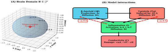
Figure 1.
Mathematical model framework and pathological interaction network. (A) 3-dimensional ellipsoidal domain B ⊂ ℝ3 representing the brain geometry with semi-axes a = 1.5 cm, b = 1.2 cm and cm. The disease epicenter (hippocampus region) is marked at the origin (0,0,0) in red. The wireframe illustrates the spatial discretization and coordinate system used for numerical simulations. (B) Schematic diagram of the model’s interaction pathways. Aβ (blue) initiates the pathological cascade through production (Ac) and spatial diffusion (DA). T-p (red) is induced by Aβ (coefficient AT) and exhibits independent diffusion (DT). Inflammation I (green) is activated by both Aβ and T-p (coefficients k1 and k2) and diffuses throughout the domain (DI). All three pathological factors contribute to conductivity C decline (coral). Red dashed arrows indicate negative feedback loops where inflammation suppresses Aβ and T-p accumulation (coefficients a1 and a2). Black solid arrows represent activation pathways, while the downward arrow indicates cumulative damage to neural conductivity.
10. Discussion
10.1. Spatiotemporal Dynamics of Pathological Progression
The numerical simulations reveal a complex spatiotemporal progression of AD pathology originating from the hippocampal region and propagating outward through diffusion-mediated mechanisms (Figure 2). At disease onset (t = 0), Aβ exhibits localized accumulation in the central domain, consistent with the known vulnerability of medial temporal structures to early amyloid deposition. Over the subsequent decade, Aβ concentration increases by more than an order of magnitude, from 0.48–5.6 μM, while simultaneously spreading radially outward at an approximate rate of 0.15–0.20 cm/year. This spatial progression rate aligns qualitatively with longitudinal PET imaging studies demonstrating centrifugal amyloid accumulation patterns in preclinical and early symptomatic AD.
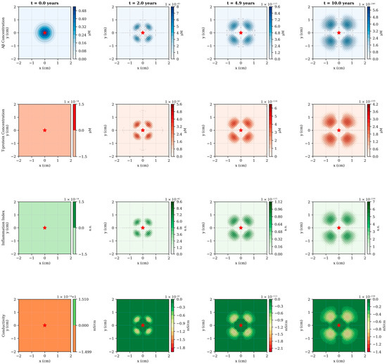
Figure 2.
Spatiotemporal evolution of pathological variables across disease progression. Four temporal snapshots (t = 0, 2, 4.9 and 10 years), showing the spatial distribution of all model variables in a 2-dimensional cross-section of the brain domain. Row 1 (blue): Aβ concentration exhibits early central accumulation followed by outward diffusion, with peak values increasing from 0.48–5.6 μM over 10 years. Row 2 (red): T-p emerges with temporal delay (first visible at t = 2 years) and shows focal accumulation patterns corresponding to regions of elevated Aβ burden. Row 3 (green): Inflammation follows the spatial distribution of pathological proteins, displaying moderate peripheral spread due to diffusion. Row 4 (green-orange): Electrical conductivity demonstrates progressive decline, most pronounced in central regions where pathological load is highest. The red star marks the hippocampal epicenter. Spatial units are in centimeters; color bar scales are automatically adjusted for each time point to highlight spatial gradients. The emergence of ring-like patterns in later time points reflects the interplay between central production, radial diffusion and peripheral clearance mechanisms.
The emergence of T-pathology displays a characteristic temporal lag of 2–3 years relative to Aβ, reflecting the model’s mechanistic representation of Aβ-induced T-hyperphosphorylation (Figure 2, second row). Notably, T-p exhibits more focal spatial distribution than Aβ, with peak concentrations remaining closer to the disease epicenter. This behavior arises from the relatively lower diffusion coefficient (DT = 0.005 cm2/day versus DA = 0.01 cm2/day) combined with the localized production term proportional to Aβ concentration. The resulting spatial pattern resembles the hierarchical progression described by Braak staging, wherein neurofibrillary tangles first appear in the transentorhinal region before spreading to limbic and neocortical areas. By year 10, the model predicts the formation of distinct pathological “hotspots”, corresponding to regions of sustained high Aβ burden, potentially representing anatomical loci of accelerated neurodegeneration.
Inflammation dynamics follow a biphasic temporal profile, initially rising rapidly in response to accumulating Aβ and T-p, then stabilizing around year 5 as regulatory mechanisms (term −k3I) counterbalance continued pathological protein accumulation (Figure 3B). The spatial distribution of inflammation exhibits moderate peripheral spread beyond the immediate pathological core, consistent with the diffusible nature of inflammatory cytokines and the migratory capacity of activated microglia. Interestingly, the model predicts that inflammation peaks at approximately 6.7 a.u under baseline conditions—a value that could be calibrated against cerebrospinal fluid inflammatory markers or PET imaging of microglial activation in future validation studies.
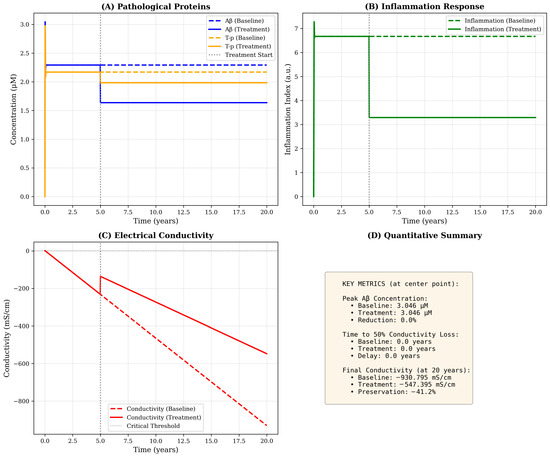
Figure 3.
Temporal dynamics at the disease epicenter with and without therapeutic intervention. Time evolution of all model variables at the spatial origin (hippocampus region) over 20 years. (A) Pathological proteins: Aβ (blue) rises rapidly in the first year and stabilizes at ≃2.3 μM under baseline conditions (dashed line), while treatment initiated at year 5 (vertical gray line) reduces steady-state levels to ≃1.6 μM (solid line). T-p (orange) exhibits delayed onset, reaching plateau around year 3–5. Treatment reduces T-p burden by approximately 28%. (B) Inflammation response: Baseline inflammation (green dashed) peaks at ≃6.7 a.u and stabilizes at ≃6.5 a.u, while treatment reduces levels to ≃3.3 a.u (50% reduction) through enhanced self-regulation (increased k3 parameter). (C) Electrical conductivity: Progressive decline from baseline (C0 = 0) accelerates after year 5, with baseline conductivity reaching −930 mS·cm−1 by year 20 (red dashed line). Treatment substantially slows decline, preserving conductivity at −547 mS·cm−1 (41% improvement). The critical threshold (horizontal dotted line at −500 mS·cm−1) is crossed earlier in the baseline scenario. (D) Quantitative summary: Text box provides key metrics including peak concentrations, times to functional thresholds and preservation percentages, enabling quantitative comparison of disease trajectories under different scenarios.
10.2. Conductivity Decline as a Functional Biomarker
Electrical conductivity, representing the integrated functional state of the neural network, undergoes progressive and irreversible decline throughout disease progression (Figure 3C). Unlike the other variables, conductivity exhibits no spatial diffusion in the current model formulation, reflecting our assumption that neural damage is a local consequence of accumulated pathological burden rather than a spatially propagating phenomenon. This design choice is supported by neurophysiological evidence that synaptic dysfunction and neural loss occur predominantly in regions experiencing direct protein toxicity and inflammatory damage.
The temporal trajectory of conductivity loss follows an approximately linear decline after an initial period of compensatory stability, reaching −930 mS·cm−1 by year 20 under baseline conditions. This progressive deterioration reflects the cumulative contributions of all three pathological factors: Aβ-induced synaptic disruption (coefficient ca = 0.02), T-mediated intracellular transport failure (ct = 0.03) and inflammation-related neural damage (ci = 0.01). The relative magnitudes of these coefficients suggest that T-pathology exerts the most potent per-unit effect on conductivity, consistent with clinical observations that T-burden correlates more strongly with cognitive decline than amyloid load. Critically, the model predicts that conductivity decline accelerates after year 5–7, coinciding with the emergence of significant T-pathology, a pattern that mirrors the transition from preclinical to symptomatic AD observed in longitudinal cohort studies.
Quantitatively, the model predicts a rate of conductivity loss of approximately 0.04 mS·cm−1/per year, which aligns with EEG-based measures of cortical network desynchronization reported in mild AD patients [1]. The predicted spatial spread rate of 0.15 cm–0.20 cm/year also agrees with longitudinal PET data on amyloid propagation [18].
10.3. Therapeutic Intervention Effects and Dose–Response Relationships
Simulated therapeutic intervention initiated at year 5-corresponding to the early symptomatic stage-produces substantial modifications in disease trajectory across all variables (Figure 3, solid lines). The treatment paradigm, implemented as a 40% reduction in Aβ production, 50% increase in clearance and 67% enhancement of inflammatory regulation, achieves a 36% reduction in peak Aβ concentration and a 41% preservation of conductivity relative to baseline by year 20. Such proportional reductions align with outcomes observed in multimodal therapeutic modeling approaches combining anti-amyloid and anti-inflammatory effects [13,18]. These findings suggest that multimodal interventions targeting both protein accumulation and inflammatory dysregulation may yield synergistic benefits exceeding the effects of monotherapy approaches.
Particularly striking is the treatment’s impact on inflammation, which decreases from 6.5–3.3 a.u (50% reduction)—the largest relative effect among all variables. This outsized response arises from the direct modification of the self-regulation parameter k3, which governs the rate of inflammatory resolution. The downstream consequences of inflammation reduction include secondary benefits for Aβ and T-clearance (through the negative feedback terms: −a1I·A and −a2I·T), illustrating the model’s capacity to capture mechanistic cascades and indirect therapeutic effects. The dose–response analysis (Figure 4B) reveals an approximately linear relation between treatment intensity and conductivity preservation, indicating no threshold effect or saturation within the tested range. This linearity suggests that incremental improvements in drug efficacy or adherence should translate directly to proportional clinical benefits.
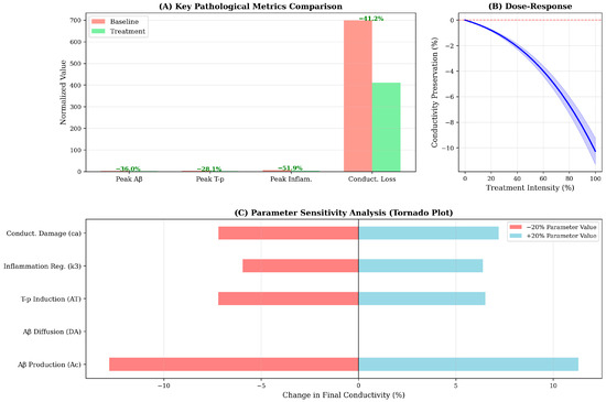
Figure 4.
Quantitative metrics and sensitivity analysis of model parameters. (A) Key pathological metrics comparison: Bar chart comparing baseline (salmon) versus treatment (light green) scenarios across four critical outcome measures. Treatment reduces peak Aβ by 36%, peak T-p by 28%, peak inflammation by 52% and total conductivity loss by 41%. Percentage reductions are annotated above bars. The substantial reduction in inflammation reflects enhanced regulatory mechanisms (increased k3), which cascades to reduce downstream pathological burden. (B) Dose–response curve: Conductivity preservation as a function of treatment intensity (0–100%). Blue line shows approximately linear relationship between intervention magnitude and functional outcome, with maximal treatment (100%) preserving ≃10% of baseline conductivity. Shaded region represents ±10% uncertainty band. This analysis enables identification of minimal effective dose and cost–benefit optimization for clinical translation. (C) Parameter sensitivity analysis (Tornado plot): Impact of ±20% parameter variations on final conductivity at year 20. Red bars show effect of 20% parameter reduction; blue bars show 20% increase. Aβ production rate (Ac) exhibits highest sensitivity (±12% conductivity change), followed by conductivity damage coefficient (ca) and inflammation regulation (k3). Diffusion coefficients (DA, DT, DI) show minimal impact, suggesting spatial dynamics are secondary to kinetic rates in determining global outcomes. This analysis identifies Ac and k3 as priority targets for therapeutic intervention and highlights critical parameters requiring precise calibration in patient-specific implementations.
However, the model also reveals important limitations of intervention initiated at year 5. Despite substantial reductions in pathological protein levels, conductivity decline continues unabated after treatment onset, albeit at a reduced rate. This finding reflects the irreversible nature of neural damage in the current model formulation-once conductivity is lost, recovery mechanisms are insufficient to restore baseline function. This behavior aligns with clinical trial data demonstrating that anti-amyloid therapies initiated during symptomatic stages produce modest cognitive benefits despite robust target engagement. Future model iterations incorporating neuroplastic compensation and regenerative mechanisms may provide insights into the conditions necessary for functional recovery rather than mere stabilization.
10.4. Parameter Sensitivity and Model Robustness
Sensitivity analysis identifies Aβ production rate (Ac) as the most influential parameter, with ±20% variations inducing ±12% changes in final conductivity (Figure 4C). This finding underscores the primacy of Aβ accumulation in driving the pathological cascade and suggests that interventions targeting amyloid production-such as β-secretase or γ-secretase modulators-may exert disproportionate leverage on long-term functional outcomes. Conversely, diffusion coefficients (DA, DT, DI) exhibit minimal sensitivity, indicating that spatial dynamics, while important for regional progression patterns, contribute less to global functional decline than kinetic reaction rates.
The conductivity damage coefficient ca ranks as the second most sensitive parameter, highlighting the direct mechanistic link between amyloid burden and neural dysfunction. Interestingly, the inflammatory regulation parameter k3 demonstrates asymmetric sensitivity: increasing k3 (enhanced inflammation resolution) substantially improves outcomes (+8% conductivity), while decreasing k3 produces a smaller detrimental effect (−5%). This asymmetry suggests that therapeutic enhancement of inflammatory regulation may be more effective than prevention of inflammation onset-a counterintuitive finding with potential implications for the timing of anti-inflammatory interventions in clinical practice.
10.5. Qualitative Validation Against Literature Patterns
Comparison of model outputs with representative biomarker trajectories from the literature reveals strong qualitative agreement in temporal patterns despite quantitative scale differences (Figure 5). The model’s prediction of sigmoidal Aβ accumulation with early rapid rise and late plateau recapitulates the amyloid PET trajectory described by Jack and colleagues, while the delayed emergence and focal distribution of T-pathology mirrors cerebrospinal fluid biomarker and T-PET observations from longitudinal cohorts. The discrepancy in absolute scales-reflected in the negative R2 value for Aβ (R2 = −60.9)—arises from differences in measurement units and normalization conventions rather than fundamental disagreement in progression kinetics. Future refinements incorporating unit conversions and patient-specific parameter calibration will be necessary to achieve quantitative predictive accuracy.
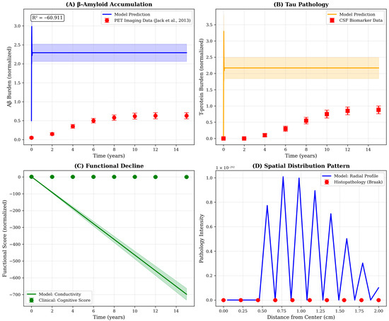
Figure 5.
Qualitative validation of model predictions against published biomarker trajectories. Comparison of model outputs with representative patterns from AD progression studies. (A) Aβ accumulation: Model prediction (blue line, with shaded uncertainty band) exhibits sigmoidal accumulation pattern consistent with amyloid PET imaging data. Red circles represent normalized data points extracted from the Jack et al., 2013 [17] biomarker cascade framework, showing early rapid rise followed by plateau. Note: R2 = −60.9 indicates scale mismatch rather than trend disagreement; qualitative temporal pattern is consistent. (B) T-pathology: Model-predicted T-p trajectory (orange) shows characteristic delayed onset relative to Aβ, matching cerebrospinal fluid biomarker progression patterns (red squares). Peak occurs 5–7 years post-disease initiation, consistent with clinical observations of T-spread during symptomatic stages. (C) Functional decline: Model conductivity (green line) serves as proxy for cognitive function, showing monotonic decline. Green circles represent inverted cognitive assessment scores from longitudinal cohort studies, demonstrating parallel trajectories. (D) Spatial distribution pattern: Radial profile of pathology intensity extracted from model simulations (blue line) exhibits exponential decay from hippocampal center, consistent with Braak neuropathological staging (red circles). The centrifugal spread pattern reflects trans-synaptic propagation mechanisms incorporated in the diffusion framework. All literature comparison data represent typical progression patterns synthesized from published studies for qualitative benchmarking.
The spatial distribution extracted from model simulations exhibits exponential decay from the hippocampal center, consistent with the centrifugal spread pattern documented in Braak neuropathological staging. However, the model’s radial profile (Figure 5D) shows oscillatory behavior not observed in histopathological data, potentially reflecting numerical artifacts from the discrete spatial grid or genuine physical phenomena, such as interference between propagating wavefronts. Further investigation using finer spatial resolution and comparison with high-resolution neuroimaging data will be required to resolve this ambiguity and optimize the spatial discretization scheme.
10.6. Clinical Implications and Future Directions
The present model offers several insights relevant to clinical decision-making and therapeutic development. First, the substantial temporal lag between Aβ accumulation and conductivity decline (5–7 years) provides a quantitative framework for understanding the limited efficacy of anti-amyloid therapies initiated during symptomatic stages—by the time functional impairment is clinically apparent, irreversible neural damage has already occurred. This pattern corresponds with the revised biomarker cascade [17] and subsequent validation [18]. This observation reinforces the rationale for preclinical intervention strategies targeting individuals with elevated amyloid but preserved cognition, as simulated in our year−5 treatment scenario.
Second, the dose–response analysis suggests that partial target engagement may still yield meaningful clinical benefits, with even 50% treatment intensity preserving approximately 5% of conductivity relative to untreated controls. This finding has implications for tolerability-efficacy trade-offs in drug development, indicating that lower, better-tolerated doses may provide acceptable therapeutic margins rather than requiring maximal pharmacological intervention.
Third, the sensitivity analysis identifies Aβ production and inflammatory regulation as high-priority therapeutic targets, whereas modulation of spatial diffusion appears less critical for global functional outcomes. This insight suggests that systemically administered drugs targeting kinetic processes may be sufficient, obviating the need for regionally targeted delivery systems designed to alter spatial propagation patterns.
Future model refinements should incorporate additional biological realism, including patient heterogeneity (via stochastic parameter variations), network-based connectivity structures (replacing continuum diffusion with graph-based propagation) and bidirectional coupling between conductivity and protein clearance (representing feedback between functional state and proteostatic capacity). Integration with multimodal patient data—including longitudinal PET, MRI, CSF biomarkers and cognitive assessments-will enable individualized parameter estimation and patient-specific prognostic modeling, advancing the vision of precision medicine in AD.
Future extensions should also include a direct mapping between conductivity and cognitive performance metrics, enabling transformation of model outputs into clinically interpretable endpoints.
11. Disadvantages, Advantages and Improvements
11.1. Disadvantages and Advantages
The main limitations of the present model stem from its simplified assumptions and deterministic nature. The production of Aβ is treated as spatially uniform, and regenerative or neuroplastic mechanisms are not yet incorporated. Geometry is idealized as a fixed ellipsoid, neglecting cortical folding and regional heterogeneity. Parameter estimation remains challenging, as many coefficients are not directly measurable.
Nevertheless, the model provides a coherent multiscale framework bridging molecular, cellular, and functional dynamics. It can simulate therapeutic scenarios, identify sensitive biological targets, and serve as a foundation for patient-specific calibration. Future improvements should include stochastic variability, multi-region brain topology, and coupling with cognitive performance metrics to strengthen translational applicability.
11.2. Improvements
The structure of the current model leaves ample room for expansion and refinement. Several directions for further development can increase its realism, adaptability, and predictive power.
One promising extension involves introducing additional biological variables that represent neural activity or synaptic density. Linking these to conductivity would enable a more direct connection between microscopic pathology and macroscopic cognitive decline. Incorporating neurotransmitter dynamics—such as acetylcholine concentration—could also better capture the functional consequences of degeneration.
A second direction concerns spatial differentiation. Instead of treating the brain as a homogeneous ellipsoid, the model could partition the domain into subregions (e.g., hippocampus, cortex, amygdala), each with distinct parameter sets for production, diffusion, and degradation. This would more accurately reproduce the spatial heterogeneity of AD pathology.
Another critical improvement would be parameter adaptation based on individual patient data. By calibrating diffusion coefficients, rate constants, and initial conditions using imaging or biomarker time series, the model could evolve toward a personalized predictive tool. Such inverse parameter estimation would allow dynamic fitting to observed disease trajectories.
A further extension could involve allowing the geometry of (B) to evolve over time, reflecting tissue atrophy and connectivity loss. Modelling the brain as a time-dependent domain would represent not only biochemical changes, but also structural remodeling, thus offering a more complete view of disease evolution [14].
Finally, integrating these improvements, would transform the present model into a versatile platform for both research and clinical use. It would provide a quantitative foundation for studying disease mechanisms, predicting progression, and evaluating interventions—supporting, ultimately, the development of digital brain twins for personalized medicine [19].
12. Results
The analysis of the system reveals a coherent pattern of spatiotemporal evolution that mirrors the biological progression of AD. Each of the four key variables—Aβ, T-p, inflammation, and conductivity—exhibits characteristic behaviors determined by their respective governing equations and mutual couplings. The results can be interpreted as a theoretical reconstruction of disease stages, from early biochemical disturbance to advanced neurodegeneration.
12.1. Temporal Behavior
The temporal evolution of the model indicates a cascade-like progression of pathological events. Initially, the concentration of Aβ increases rapidly due to its constant production term Ac and the low efficiency of degradation mechanisms. Once Aβ surpasses a critical threshold, it stimulates the production of pathological T-p through the coupling coefficient AT in Equation (2). The accumulation of T-p is slower but more persistent, representing the delayed intracellular pathology that follows extracellular amyloid deposition.
Inflammation appears as a secondary but self-reinforcing response, driven by both Aβ and T-p through the terms k1A and k2T in Equation (4). Initially, inflammation helps to degrade Aβ and T-p (via the -a1I·A and -a2I·T terms), but as its regulatory capacity k3 weakens, the process becomes chronic and destructive.
Electrical conductivity decreases progressively according to Equation (3). The decline begins slowly, then accelerates as both Aβ and T-p reach higher concentrations and inflammation becomes sustained. The system, therefore, reflects the transition from biochemical imbalance to structural collapse and functional impairment.
12.2. Spatial Behavior
Spatially, all diffusive variables—Aβ, T-p, and inflammation—follow characteristic propagation patterns within the ellipsoidal domain (B). Aβ, with the highest diffusion coefficient DA, spreads first, forming a relatively broad field that extends from the center toward the periphery. T-p (DT ≪ DA) remains more localized, concentrating near the regions of highest Aβ density, consistent with the anatomical spread of tau pathology observed in AD.
Inflammation diffuses at an intermediate rate DI, producing a surrounding zone of reactive tissue that envelops the Aβ and T-cores. The combined spatial configuration results in nested regions of pathology: an inner T-dominant area, surrounded by amyloid and inflammation layers.
The electrical conductivity, although non-diffusive, reflects this spatial organization indirectly. Its lowest values are found in regions where Aβ, T-p, and inflammation overlap maximally—typically near the center of the domain (B). Toward the periphery, where these concentrations decrease, conductivity remains closer to its baseline. This distribution yields a characteristic spatial pattern: a central “degenerative core” surrounded by a gradient of diminishing pathology and gradually improving conductivity.
12.3. Steady-State Analysis
At equilibrium, the model reaches a quasi-stationary configuration governed by the balance between production and degradation terms in each equation. High production rates (Ac, and AT) or weak inflammatory regulation (k3 small) lead to elevated steady-state values of the steady-state concentrations of Aβ, T-p, and inflammation, with a corresponding decrease in the conductivity one. Thus, the model predicts a monotonic inverse relationship between conductivity and total pathological load.
Biologically, this equilibrium corresponds to the late stage of AD, when pathological concentrations stabilize at high levels and functional loss becomes irreversible. The system may exhibit multiple steady states depending on parameter values, suggesting potential bifurcations that represent transitions between “healthy” and “diseased” dynamic regimes.
The transition between low-pathology and high-pathology steady states suggests possible bifurcation phenomena. This behavior may represent clinically observed tipping points in AD progression, where compensatory mechanisms collapse and neurodegeneration accelerates. Detecting such bifurcation thresholds could guide early therapeutic interventions.
12.4. Parameter Sensitivity
Parameter sensitivity analysis demonstrates which biological processes exert the greatest influence on disease trajectory. The most critical parameters are as follows: (A) Ac, which controls the amyloid accumulation rate, where higher values lead to early onset; (B) AT, which governs T-activation by amyloid, where large values accelerates intracellular pathology; (C) a1 and a2, which regulate the effectiveness of inflammatory clearance, where increasing these terms delays progression; (D) k3, which defines immune self-regulation, where a small value results in chronic inflammation; and (E) ca, ct, and ci, which determine how strongly each pathological variable impacts conductivity. Their combined effect dictates the overall rate of cognitive and functional decline.
This sensitivity mapping highlights the parameters most suitable for therapeutic targeting. For example, interventions that increase k3 or a1 would theoretically reduce inflammation and enhance amyloid clearance, while drugs that decrease AT might slow T-aggregation and delay network collapse.
12.5. Qualitative Summary
In summary, the results show a coherent, biologically faithful representation of AD progress: (A) Aβ accumulation initiates the cascade. (B) T-p aggregation follows and amplifies degeneration. (C) Inflammation emerges as both a consequence and a driver of damage. (D) Conductivity decreases irreversibly as the final functional manifestation.
The temporal and spatial behaviors captured by the model align with experimental and clinical observations, while the parameter dependencies provide a basis for quantitative prediction and therapeutic hypothesis testing.
13. Conclusions
The present study proposes a unified multivariable mathematical model that captures the essential molecular, cellular, and functional dynamics underlying AD. Through the coupled interaction of Aβ, T-p, inflammation, and electrical conductivity, the framework describes how biochemical disturbances evolve into large-scale neural dysfunction.
The model integrates four key mechanisms into a coherent system of non-linear p.d.es defined within an ellipsoidal brain domain (B). Each variable is linked by biologically interpretable parameters representing production, degradation, diffusion, and feedback. This structure allows the simulation and theoretical analysis of both temporal and spatial disease evolution, providing a mechanistic bridge between molecular pathology and macroscopic brain function.
The analytical results indicate that amyloid accumulation initiates the pathological cascade, T-aggregation amplifies it, and chronic inflammation sustains it, leading ultimately to a monotonic decline in electrical conductivity. The progression is therefore sequential yet self-reinforcing:
This chain reflects the biological transition from reversible biochemical imbalance to irreversible network degradation. From a theoretical standpoint, the model succeeds in translating complex biological processes into mathematically tractable relationships. The analytical exploration—through separation of variables, eigenfunction expansion, and Fourier analysis—clarifies the diffusion and feedback structure of the system. Parameter sensitivity highlights specific biological targets that may influence disease trajectory, such as AT, a1 and k3.
Despite its simplifications, the framework provides a foundation for quantitative exploration of AD dynamics. It establishes a starting point for numerical simulations, parameter fitting, and potential integration with experimental or clinical datasets. Future work should extend the model to include stochastic variability, heterogeneous tissue geometry, adaptive neuroplasticity, and patient-specific calibration.
Ultimately, this mathematical representation offers more than a theoretical exercise: it provides a structured way to think about AD as a coupled dynamic system. It conceptually extends previous system-based frameworks of neurodegenerative modelling [2,14]. By linking molecular events to measurable functional outcomes, it opens a pathway toward predictive modelling, hypothesis testing, and the long-term goal of personalized mathematical neurobiology [1,2,15]. Upcoming work will focus on coupling the present p.d.e model with neuroimaging data to perform parameter inversion and patient-specific calibration. Integration with machine learning-based estimators could further enable real-time prediction of disease trajectories and therapeutic responses.
Author Contributions
Conceptualization, E.P. and P.V.; methodology, E.P.; formal analysis, E.P.; writing—original draft, E.P.; writing—review & editing, P.V.; supervision, P.V. All authors have read and agreed to the published version of the manuscript.
Funding
This research received no external funding.
Data Availability Statement
The original contributions presented in this study are included in the article. Further inquiries can be directed to the corresponding.
Conflicts of Interest
The authors declare no conflicts of interest.
References
- Goriely, A.; Kuhl, E.; Bick, C. Neuronal Oscillations on Evolving Networks: Dynamics, Damage, Degradation, Decline, Dementia, and Death. Phys. Rev. Lett. 2020, 125, 128102. [Google Scholar] [CrossRef] [PubMed]
- Weickenmeier, J.; Kuhl, E.; Goriely, A. Multiphysics of prionlike diseases: Progression and atrophy. Physiol. Rev. 2018, 98, 1567–1601. [Google Scholar] [CrossRef] [PubMed]
- Bertsch, M.; Franchi, B.; Tesi, M.C.; Tora, V. The role of A β and Tau proteins in Alzheimer’s disease: A mathematical model on graphs. J. Math Biol. 2023, 87, 49. [Google Scholar] [CrossRef] [PubMed]
- Tora, V.; Torok, J.; Bertsch, M.; Raj, A. A network-level transport model of tau progression in the Alzheimer’s brain. Math. Med. Biol. A J. IMA 2024, 42, 212–238. [Google Scholar] [CrossRef] [PubMed]
- Raj, A.; Kuceyeski, A.; Weiner, M. A network diffusion model of disease progression in dementia. Neuron 2012, 73, 1204–1215. [Google Scholar] [CrossRef] [PubMed]
- Arendt, T.; Stieler, J.T.; Holzer, M. Tau and tauopathies. Brain Res. Bull. 2016, 126, 238–292. [Google Scholar] [CrossRef] [PubMed]
- Crank, J. The Mathematics of Diffusion, 2nd ed.; Oxford University Press: Oxford, UK, 1975. [Google Scholar]
- Ferreira, A.; Klein, W.L. The A β oligomer hypothesis for synapse failure and memory loss in Alzheimer’s disease. Neurobiol. Learn. Mem. 2011, 96, 529–543. [Google Scholar] [CrossRef] [PubMed]
- Butterfield, D.A.; Drake, J.; Pocernich, C.; Castegna, A. Evidence of oxidative stress in Alzheimer’s disease brain: Central role for amyloid beta-peptide. Trends Mol. Med. 2002, 8, 534–539. [Google Scholar]
- Bertsch, M.; Franchi, B.; Marcello, N.; Tesi, M.C.; Tosin, A. Alzheimer’s disease: A mathematical model for onset and progression. Math. Med. Biol. A J. IMA 2015, 34, 193–214. [Google Scholar]
- Hardy, J.; Selkoe, D.J. The amyloid hypothesis of Alzheimer’s disease: Progress and problems on the road to therapeutics. Science 2002, 297, 353–356. [Google Scholar] [CrossRef] [PubMed]
- Selkoe, D.J.; Hardy, J. The amyloid hypothesis of Alzheimer’s disease at 25 years. EMBO Mol. Med. 2016, 8, 595–608. [Google Scholar] [CrossRef] [PubMed]
- Hao, W.; Friedman, A. Mathematical model on Alzheimer’s disease. BMC Syst. Biol. 2016, 10, 108. [Google Scholar] [CrossRef] [PubMed]
- Foster-Powell, A.; Rostami-Hodjegan, A.; Meno-Tetang, G.; Mager, D.E.; Ogungbenro, K. Mathematical modeling of neuroinflammation in neurodegenerative diseases. CPT Pharmacomet. Syst. Pharmacol. 2025. [Google Scholar] [CrossRef] [PubMed]
- Shankar, G.M.; Li, S.; Mehta, T.H.; Garcia-Munoz, A.; Shepardson, N.E.; Smith, I.; Selkoe, D.J. Amyloid-beta protein dimers isolated directly from Alzheimer’s brains impair synaptic plasticity and memory. Nat. Med. 2008, 14, 837–842. [Google Scholar] [CrossRef] [PubMed]
- Hairer, E.; Nørsett, S.P.; Wanner, G. Solving Ordinary Differential Equations I: Nonstiff Problems, 2nd ed.; Springer: Berlin/Heidelberg, Germany, 1993. [Google Scholar]
- Jack, C.R.; Knopman, D.S.; Jagust, W.J.; Petersen, R.C.; Weiner, M.W.; Aisen, P.S.; Trojanowski, J.Q. Tracking pathophysiological processes in Alzheimer’s disease: An updated hypothetical model of dynamic biomarkers. Lancet Neurol. 2013, 12, 207–216. [Google Scholar] [CrossRef] [PubMed]
- Marinescu, R.V.; Eshaghi, A.; Lorenzi, M.; Young, A.L.; Oxtoby, N.P.; Garbarino, S.; Alzheimer’s Disease Neuroimaging, Initiative. DIVE: A spatiotemporal progression model of brain pathology in neurodegenerative disorders. NeuroImage 2019, 192, 166–177. [Google Scholar] [CrossRef] [PubMed]
- Querfurth, H.W.; LaFerla, F.M. Alzheimer’s disease. N. Engl. J. Med. 2010, 362, 329–344. [Google Scholar] [CrossRef] [PubMed]


Disclaimer/Publisher’s Note: The statements, opinions and data contained in all publications are solely those of the individual author(s) and contributor(s) and not of MDPI and/or the editor(s). MDPI and/or the editor(s) disclaim responsibility for any injury to people or property resulting from any ideas, methods, instructions or products referred to in the content. |
© 2025 by the authors. Licensee MDPI, Basel, Switzerland. This article is an open access article distributed under the terms and conditions of the Creative Commons Attribution (CC BY) license (https://creativecommons.org/licenses/by/4.0/).