Abstract
Background: Liver transplantation is the most effective curative treatment for patients with hepatocellular carcinoma. Due to the scarcity of cadaveric donor livers, several selection criteria have been established; however, these criteria are highly restrictive. In this study, we compare alternative selection tools with the standard selection criterion, the Milan Criteria. We conducted a cost-effectiveness analysis from the perspective of the U.S. healthcare system to determine which criterion provides the greatest benefit to the health system. Methods: An innovative non-homogeneous Markov model was developed to simulate the health trajectories of patients with hepatocellular carcinoma who underwent liver transplantation over five years. The model incorporated time-dependent transition probabilities, enabling the simulation to capture the evolving risks of recurrence and mortality. Transition probabilities, costs, and QALYs were obtained from published studies, while recurrence probabilities were estimated using the Kaplan–Meier method based on a cohort of 149 patients. We evaluated mean recurrence-free survival, life years gained, quality of life, and the incremental cost-effectiveness ratio (ICER) relative to the Milan Criteria. Results: HepatoPredict yielded the most significant benefits but incurred higher total costs than the other criteria. The ICERs of HepatoPredict Class I and Class II relative to the MC were $14,689.58/QALY and $39,542.98/QALY, respectively. Both values were below the cost-effectiveness threshold (U.S. GDP per capita: $81,632.25/QALY), indicating that HepatoPredict is cost-effective in the U.S. healthcare system. Conclusions: HepatoPredict stands out as the most cost-effective criterion and optimises organ allocation, an especially important consideration given the scarcity of donor livers. This represents a substantial advantage for healthcare institutions.
Keywords:
non-homogeneous Markov model; survival analysis; cost-effectiveness analysis; Hepatocellular Carcinoma (HCC); selection criteria for liver transplantation MSC:
62M05; 62N02; 62P10; 62P20
1. Introduction
Liver cancer is the sixth most common cancer in the world, with 866,136 new cases in 2022, and has the third highest mortality rate, with 758,725 deaths [1]. Hepatocellular Carcinoma (HCC) is the most common type of primary cancer of the liver, representing 80–90% of all cases [2,3].
Liver cancer incidence is distributed in Eastern Asia (50%), South-Eastern Asia (12%), South Central Asia (6.9%), Northern America (5.6%), Northern Africa (3.7%) and Western Europe (3.2%) [1]. HCC is associated with many sociodemographic characteristics (age, sex, and other factors). Advancing age is a significant risk factor, as age-specific incidence rates are highest in individuals over 70 years [4]. Studies report higher rates of HCC by racial or ethnic groups, such as non-Hispanic white, Asian/Pacific Islander, and Hispanics (people from Spanish-speaking countries) [5]. Another risk factor is sex, with a higher prevalence in the male population (≈69%) [6].
There are many classification systems for patients with HCC, but the most widely used is the Barcelona Clinic Liver Cancer (BCLC) staging system. This classification system aims to help guide treatment decisions and predict the prognosis of patients with HCC, meaning predicting if a patient will relapse or not after the transplant. This classification is based on tumour burden, liver function, and physical status. It has been refined by the Alpha-Fetoprotein (AFP), ALBI (albumin-bilirubin) score, Child-Pugh and MELD (model for end-stage liver disease) score. In general, patients in early or intermediate stages of the disease are good candidates for liver transplantation [7].
Depending on the stage of the disease and the patient’s overall condition, various treatment options are available: liver resection, liver transplant (LT), ablation, trans-arterial chemoembolization (TACE), systemic treatment, and best supportive care [7]. Among these, liver resection and LT are recognised as the only curative intent treatments for HCC patients [8,9].
LT is the best curative treatment for HCC patients with/without chronic liver disease, with better overall survival and recurrence-free survival (RFS) rates than other treatment options [8]. However, liver donors—more specifically, cadaveric livers—are a scarce resource [10]. To ensure their efficient allocation, over the past three decades, selection criteria have been developed to identify patients with HCC most suitable for transplantation, namely those at lower risk of relapse after LT [11]. The major limitation of these criteria is their restrictive nature, which results in a small number of patients meeting the requirements and/or the exclusion of many patients with a favourable prognosis [12].
The most frequently used criteria are the Milan Criteria (MC), the University of California, San Francisco (UCSF) criteria, the Up-to-7 (UP7) criteria, the AFP Model, and MetroTicket 2.0 (MT2.0). Most of these criteria only use clinical parameters (number of tumours and tumour size), derived from preoperative imaging (Table 1). Consequently, they do not account for HCC aggressiveness, which can vary among patients with identical clinical profiles, thereby limiting their ability to accurately predict prognosis. In addition to clinical parameters, the AFP Model and the MT2.0 criteria also incorporate a biomarker (AFP levels) [13], which has demonstrated prognostic value for HCC in non-transplant patients [14]. Details about the selection criteria under study can be found in Table 1. Each criterion selects patients according to its own requirements/rules, resulting in different patient selections for transplantation.

Table 1.
Inclusion criteria for classifying HCC patients. Clinical parameters refer only to liver tumours, with size corresponding to diameter.
HepatoPredict (HP) is a medical prognostic device developed by Ophiomics [19], a company dedicated to advancing precision medical technologies in oncology. In its HP.AI version 2, the device combines three clinical variables related to the tumour (number of tumours, largest tumour size (diameter), and total tumour volume) with the tumour gene signature of four molecular biomarkers (CLU, DPT, SPRY2, CAPSN1) obtained from a tumour biopsy. This product integrates two distinct algorithms—one for optimised precision and the other for recall—to classify patients into three classes: HP-ClassI, HP-ClassII (good prognosis) and HP-Class0 (bad prognosis). However, the use of HP requires a tumour biopsy on the patient to obtain a tumour gene signature, making it the only pre-transplant prognostic tool that requires a biopsy [12].
Health economic models provide a structured framework for comparing the costs and outcomes of alternative interventions, thereby supporting evidence-based decisions on both patient-level treatment choices and resource allocation. In this study, we employ such a model to assess the cost-effectiveness of the selection criteria mentioned above in comparison with the MC, which is the most widely used benchmark for determining eligibility for LT. The analysis is based on U.S. data, as this source provides more reliable information to support the study. It is conducted from the healthcare system perspective to determine which criteria improve cost-effectiveness, enhance the patient journey, and are economically feasible to implement.
In this study, we developed a time-dependent Markov process to model the health trajectories of patients with HCC who underwent LT over a five-year period. An innovative procedure was introduced for constructing the elementary transition matrices, allowing the model to incorporate time-varying transition probabilities and more accurately reflect patients’ evolving health status. This framework enabled the simulation of patient distribution across health states and the computation of key health and cost-effectiveness measures commonly used in health economics. The study highlights the importance of adopting rigorous mathematical modelling to support reliable health economic evaluations. To the best of the authors’ knowledge, this is the first study of its kind to evaluate and identify the most effective selection criterion for LT in patients with HCC.
The article is structured as follows. Section 2 outlines the methodology for the cost-effectiveness analysis, including the process for obtaining the relevant data and parameters. Section 3 presents the main findings, while Section 4 discusses the results, highlights the study’s limitations, and outlines directions for future research. Section 5 concludes with the key findings and their potential contributions to society.
2. Methodology
2.1. Clinical and Probabilistic Assumptions
The study was conducted under a set of clinical and probabilistic assumptions, detailed as follows:
- (i)
- Adult patients (≥18 years old);
- (ii)
- Patients with early to intermediate HCC;
- (iii)
- Patients without regional nodal or distant metastases;
- (iv)
- Patients without comorbidities that could affect quality of life or life expectancy;
- (v)
- Molecular analyses performed on explant specimens (diseased liver removed from transplanted patients) were equivalent to molecular analyses performed on a biopsy sample (pre-transplant);
- (vi)
- The probability of mortality for relapsed patients who received different treatments (such as resection, ablation, or systemic therapy) was equal to that of patients who only received systemic therapy;
- (vii)
- The probability of mortality for patients without recurrence was assumed to be equal to the all-cause mortality of HCC patients who underwent transplantation in the U.S. during 2017;
- (viii)
- The probability of transplant-related mortality was not applied to patients who relapsed within the first three months;
- (ix)
- Costs did not include all expenses related to hospital infrastructure, such as laboratories;
- (x)
- In any given month, the probability of a patient being in a specific health state depends solely on the patient’s health state in the preceding month (Markov property).
Although assumption (iv) may appear restrictive, it was primarily motivated by the need to reduce confounding factors that could affect the mathematical model and by limited data availability. In particular, excluding patients with comorbidities avoids confounding effects that would otherwise hinder the assessment of the true impact of the selection criteria for liver transplantation. Moreover, as the transition probabilities were derived from published studies that do not distinguish between treatments or comorbidities, it was not possible to relax this assumption in the present work.
Regarding assumption (vi), only the effect of systemic therapy was considered in the probability of mortality for patients who relapsed, due to the lack of available data. Although this assumption does not fully reflect the complexity of real-world treatment pathways, it represents a conservative simplification, as systemic therapy is typically prescribed for patients at higher risk of disease dissemination and is generally associated with lower survival rates. Consequently, the cost-effectiveness analysis was conducted under a worst-case scenario for post-relapse outcomes, which we consider an appropriate approach in health economic evaluation.
2.2. Health Economic Model: Markov Model
Health economic models—such as decision trees, Markov models, and microsimulation approaches—provide a mathematical framework for comparing the costs and health outcomes of alternative interventions. They offer a systematic means of evaluating cost-effectiveness, estimating budget impact, and positioning an intervention relative to competing strategies [20,21]. Key measures of outcomes include Life Years Gained (LYG), Recurrence-Free Survival (RFS) and quality-adjusted life years (QALYs), which quantify the survival advantage associated with LT. By integrating parameters such as utilities, transition probabilities, and costs, these models support the efficient allocation of healthcare resources and the quantitative comparison of interventions.
Markov models have been extensively used in the field of health economics in order to study the evolution of various diseases and conditions. In a recent database review, it was found that Markov models were the chosen assessment technique in 49% of the manuscripts surveyed [22]. Markov model applications range from evaluating a ligament injury prevention program for amateur football players in Australia [23], to assessing a combination of therapies for relapse patients with multiple myeloma [24], and to estimating the cost-effectiveness of early screening strategies for newborn hearing impairment [25]. In the particular case of hepatocellular carcinoma, two studies conducted in Australia and in the United Kingdom have used Markov modelling the assess and evaluate the cost-effectiveness of strategies designed to prevent and/or reduce the incidence of liver-related conditions, namely routine surveillance of patients with compensated cirrhosis [26] and non-invasive tests for high-risk metabolic dysfunction-associated steatotic liver disease [27].
In this study, we used a Markov model to simulate the clinical progression and economic consequences associated with the alternative selection criteria for LT under evaluation. This modelling approach allows for the representation of transitions between mutually exclusive health states over time, thereby capturing both the stochastic nature of disease evolution and the accumulation of costs and health outcomes throughout the follow-up period.
In brief, Section 2.2.1 defines the Markov chain representing the patient’s journey after LT, with particular emphasis on the transition probabilities that rule the movement between health states over time. Section 2.2.2 describes how costs and QALYs are assigned to each health state to quantify the associated economic and health outcomes, thereby enabling the cost-effectiveness analysis. The computation of two additional measures, LYG and RFS, is also detailed.
2.2.1. Formulation of the Markov Model
In this study, we developed a non-homogeneous Markov model from a healthcare system perspective over a five-year horizon (60 months). This horizon was selected because evidence from studies comparing selection criteria for HCC patients undergoing LT indicates that the most pronounced survival benefits in post-transplant outcomes occur within this period [14,16,17,18,28,29,30]. The Markov model was chosen because it represents the evolution of a system over time through a defined set of states, with transitions between states allowing the comparison of costs and benefits of health interventions involving recurrent events [31,32]. Each Markov cycle lasted one month, simulating the outcomes of patients with HCC undergoing LT, resulting in a total of 60 cycles under consideration.
The health economic model developed in this work simulates the post-LT journey of patients through three distinct health states, defined by clinical descriptors (Figure 1). The aim is to investigate the effect of seven selection criteria (HP-ClassI, HP-ClassII, MC, UCSF, UP7, AFP Model, and MT2.0) for patients with HCC undergoing LT, classifying these hypothetical patients as either within or outside each criterion.
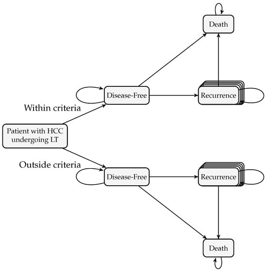
Figure 1.
Health states in the Markov model. Each square represents a state, with arrows indicating monthly transitions, including remaining in the same state. The state Recurrence is a tunnel state.
The rationale underlying the Markov model depicted in Figure 1 can be summarized as follows. At baseline (), all patients were assumed to have undergone LT. Accordingly, the model incorporated the hospital’s costs associated with transplantation, including pre-LT examinations, hospitalization, nursing appointments, and the transplantation procedure itself. In the HepatoPredict scenario, patients underwent an additional biopsy and were tested using the HP kit. All patients entered the model in the Disease-Free state. Patient assessment and follow-up occur at regular one-month intervals. During the first three months post-transplantation, patients received follow-up treatment instead of surveillance, regardless of whether they were in the Disease-Free or Recurrence state. While in the Disease-Free state (i.e., LT was performed with curative intent in patients with HCC, who were considered disease-free after transplantation until potential tumour recurrence occurred), patients were monitored monthly (surveillance). They could either remain Disease-Free, transition to the Death state due to causes unrelated to cancer recurrence, or relapse (that is, develop hepatic or extrahepatic recurrence) and move to the Recurrence state. Patients who relapsed received systemic therapy for the first three months, followed by monthly monitoring until death or the end of the study. In this model, relapse was assumed incurable with systemic therapy; thus, patients either remained in the Recurrence state (living with recurrent cancer) or transitioned to the Death state due to treatment-related mortality, cancer progression, or other causes. Upon death, the model accounted for the hospital costs associated with the patient’s death. The state Death is, therefore, an absorbing state. Note that this state includes a self-transition to ensure that the corresponding row of the one-step transition probability matrix sums to one, thereby preserving the stochastic property of the matrix. As shown in Figure 1, our Markov process takes discrete values with state space,
The Recurrence state is represented as a tunnel state of 49 substates to track the number of months a patient remains in it. This is necessary because survival probabilities vary annually and treatments differ between the first three months and subsequent months. Beyond month 49, additional tunnel states are unnecessary, as survival stabilises and no further alternative treatments are applied.
The same state space is applied to patients both within and outside the criteria; accordingly, we use the nomenclature and to represent Within Criteria and Outside Criteria, respectively. So, the state space for patients within the criteria is defined as
whereas for patients outside the criteria, it is
Hence, the global state space is given by and
The set of all criteria under consideration, U, is
Patients were evaluated every month over a 5-year period (60 months). Hence, the parameter space is a finite set. Let denote the Markov process describing the health evolution of patients in the post-LT for HCC under criterion This process characterises the transitions of individual patients between the health states under study over time. To obtain the distribution of patients across states at each monthly cycle t, we will introduce in Section 2.2.2 the state vector , which summarises the proportion of patients in each state at time t.
Returning to the Markov process , the one-step transition probabilities are time-dependent and are represented by the matrix , where
with representing the probability of transitioning from state i at month t to state j at month under criterion c. The one-step transition probability matrix is stochastic, hence .
It is important to note that the inclusion of tunnel states partially relaxes the Markov assumption that a patient’s health in a given month depends solely on the previous month’s state (Equation (1)). By explicitly modelling the time since entry into the recurrence state, the model accounts for the duration since the first month of recurrence and implicitly tracks the passage of time as patients progress deterministically through the tunnel states. Moreover, Equation (1) also allows for time-dependent transitions. Taken together, the use of tunnel states and time-dependent transitions provides a more accurate and clinically meaningful representation of disease evolution.
Figure 2 presents the transition diagram of the Markov model under study. Next, we analyse in detail the transition probabilities under consideration.
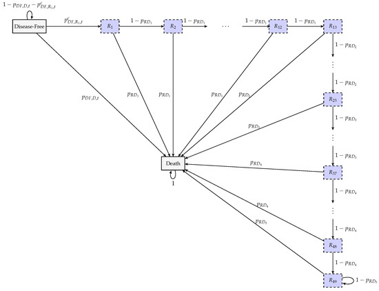
Figure 2.
Elementary transition diagram between states of the Markov chain. The dashed purple squares are the tunnel states associated with the Recurrence state.
The transition probability from the recurrence state to death varies annually following relapse, yielding five distinct death probabilities over the 5-year horizon under analysis. These probabilities are assumed to remain constant across months, invariant across criteria, and identical for patients both within and outside the criteria. Formally, we get
where
that is, represents the probability that a patient who has relapsed dies k years later.
Next, we analyse the probability that a patient with recurrence stays in the Recurrence state in the next month. This means that from month t to , the patient moves from the tunnel state to (if the patient is within criteria), or from to (if the patient is outside criteria), with this probability being identical across all criteria and not varying over time. These probabilities depend on the duration of time since the recurrence occurred. To capture this dependence, tunnel states were introduced within the general Recurrence health state, enabling the model to track the number of months a patient has survived with recurrence. Because the survival probability remains constant from the 49th to the 60th month after recurrence, no additional tunnel states are required for this interval; patients remain in state or until the end of the study, or until they die. Formally, the transition probability between two consecutive recurrence states is defined as
The transition probability from the disease-free state to death varies over time. During the first three months after LT, this probability reflects the risk of postoperative complications and is identical across all criteria. From the fourth month onwards, it represents mortality due to causes unrelated to HCC or postoperative complications, which is common to all criteria. This probability is time-dependent and changes annually. Formally,
where denotes the probability of death from transplant-related causes after LT, and represents the probability of transitioning from the disease-free state to death in the kth year after LT due to causes unrelated to HCC.
The probability of transitioning from the disease-free state to recurrence depends on the selection criterion for LT. This probability plays a key role in differentiating the criteria studied in this work, as all other transition probabilities are independent of the criterion being evaluated. In this context, it is crucial to introduce the probability of recurrence-free survival (RFS) from month t to , denoted by (for a patient within the criterion c); and (for a patient outside the criterion c), Therefore, the probability of transitioning from the state Disease-Free to the tunnel state , , is given by
Finally, the probability of remaining disease-free from month t to is given by,
The probabilities defined in Equations (2)–(5) constitute the one-step transition probabilities depicted in Figure 2.
All transition probabilities were derived from published sources, except for the probability of transition from the disease-free state to the first recurrence tunnel state, (Equation (5)). In this latter case, the probabilities were estimated using data from a patient cohort comprising individuals from two different countries. As RFS is the key parameter distinguishing the different criteria, this probability will also be considered here as a measure to evaluate the effectiveness of the various criteria in determining eligibility for LT. The methodology of the estimation procedures is described in Section 2.2.2.
Although time-dependent Markov processes can incorporate temporal features such as trend, seasonality, and short-term fluctuations, this extension was not pursued due to the absence of time-series data describing post-transplant trajectories of patients with HCC and the limited evidence available in the literature.
2.2.2. Costs and Health Economic Measures
Next, we analyse how costs and utilities are assigned to each health state in the Markov model to estimate total costs and quality-adjusted life-years (QALYs) per annual cycle over a 5-year time horizon. The results are reported from the U.S. healthcare system perspective. Costs and QALYs are discounted at an annual rate of 3% to reflect the present value of future costs and health benefits [33]. Therefore, the values were divided by the appropriate discount rate, ensuring that all costs were aligned to the same time horizon, December 2023.
To calculate the total costs and health outcomes, we simulated a cohort of n patients and followed their health trajectories over time across the different states of the Markov model. First, we defined the initial state vector, , which specifies whether patients were within or outside each criterion. The proportion of patients within each criterion was established according to the respective percentages observed in the cohort under study (see Section 3.1 for the details). The model was then simulated to determine the evolution of the cohort across health states over time. At each monthly cycle t, the distribution of patients was obtained by iteratively multiplying the initial state vector by the transition matrices, taking into account that, in a time-dependent Markov chain, the probability of being in a given state at time t results from the cumulative product of all previous transition matrices. More precisely,
Thus, the 102-dimensional random vector , represents the distribution of patients across the state space S at month t, t = 1, …, 60. To facilitate subsequent computations, we collected all these vectors into the random matrix of patient distribution trajectories, , of dimensions , representing the complete trajectory of patient distribution across all states and cycles:
These patient distributions at each time point are subsequently combined with the costs and utilities assigned to each state, allowing for the computation of total costs, LYG, RFS and QALYs.
The calculation of the total costs for the month t for all patients under criterion c requires consideration of all cost components included in the health economic model. The initial costs at correspond to the expenses associated with the transplantation procedure. These costs may be higher under the HP criterion, as this involves additional expenditures relative to the other criteria under analysis. For the five-year follow-up period, the total costs also encompass expenses incurred throughout the post-transplant phase, including surveillance, systemic therapy, and death-related costs. During the first three months after LT, these also encompassed extended post-operative care. More precisely, the initial costs are given by:
The total costs for months take the form,
For month the total costs are given by,
- : Cost of the HP kit plus the labour required to perform it.
- : Cost of the ultrasound-guided liver biopsy.
- : Minimum cost needed before transplantation.
- : Cost related to liver transplant.
- : Costs of hospitalisation and nursing care immediately after the transplant.
- : Monthly cost of patient follow-up.
- : Monthly cost of systemic therapy.
- : Cost incurred by the hospital when a patient dies.
- : Cost of the first month related to extra post-operative care.
- : Costs of the second and third months related to extra post-operative care.
Additionally, represents the monthly discount rate for costs obtained from an annual rate of 3%,
Thus, the average initial cost () and the annual costs () for criterion are given by:
Finally, the average total cost for criterion takes the form,
The quality-adjusted life year (QALY) is a widely used indicator in health economics that captures the trade-off between length and quality of life. Quality of life is quantified by assigning patients’ preference values, known as utilities, to different health states. In this work, we assume that the utility function takes values in the interval , where 0 corresponds to the utility of death and 1 represents the utility of perfect health. Accordingly, QALYs are computed as the product of the utility of each health state and the time spent in that state. In this study, the total QALYs for all patients under each criterion were computed by accounting for the distribution of patients across health states in each cycle and applying a time-dependent monthly discount rate. Each health state was assigned a monthly QALY weight equal to one-twelfth of its corresponding annual value.
In this study, we primarily used the QALYs derived from Chong et al. [34], in which health utility values were obtained by combining the standard gamble and visual analogue scale techniques with responses from the EQ-5D and Health Utilities Index Mark 3 (HUI3) questionnaires.
During the first three months, patients experienced the same quality of life in the post-operative period, regardless of whether they were in the Disease-Free or Recurrence health state. Hence, the total QALYs for the first three months, , take the form,
For the subsequent months, the total QALYs, are defined as:
- : Monthly QALY in the first three months post-transplant.
- : Monthly QALY of a cancer-free patient after transplantation.
- : Monthly QALY for a patient experiencing recurrence after transplantation.
- : represents the monthly discount rate for QALYs (annual rate of 3%).
The average total QALY for criterion thus takes the form,
The Incremental Cost-Effectiveness Ratio (ICER) evaluates the cost-effectiveness of a new treatment relative to the standard of care. It is calculated as the difference in costs divided by the difference in QALYs, representing the additional cost per QALY gained with the new intervention. QALYs were selected as the measure of treatment benefit due to their widespread use in health economic evaluations. In this study, MC was designated as the reference intervention, as it was the first selection criterion developed and remains in use in some regions. The ICER for criterion c, , was computed as follows,
where represent the cost and QALY associated with criterion c, respectively.
To assess whether the ICER is acceptable, we compared it with the willingness-to-pay (WTP) threshold based on the U.S. healthcare system, which in this study is $81,632.25 [35]. If the ICER is below this threshold, the intervention associated with criterion c is considered cost-effective. Conversely, if it exceeds the threshold, the intervention may be considered too costly in relation to the health outcomes it provides.
Life Years Gained (LYG) and Recurrence-Free Survival (RFS) are also standard outcome measures commonly used to compare different selection criteria for a given intervention. LYG captures life extension due to the intervention without weighting for quality of life during the follow-up period. Some organisations recommend presenting both QALYs and LYGs in the analysis to determine if the quality of life has a significant impact on net benefit [36]. LYG is particularly relevant here, as life extension is the primary health outcome in LT decisions based on a given criterion.
In this work, we calculated the average of LYG for our simulated patients from the Markov model within and outside the criterion denoted by and , respectively, using the following equations:
To assess the effectiveness of the different criteria for selecting patients for LT, it is also essential to analyse RFS in order to evaluate patients’ disease-free survival time after LT. Based on our simulated patients from the Markov model with size n, we computed the total months of RFS according to the following equations:
where
- -
- , : total months of RFS for all patients who did not experience recurrence, within and outside criterion c, respectively;
- -
- , : total months of RFS for all patients who experienced recurrence, within and outside criterion c, respectively;
- -
- , : total months lost due to recurrence, for all patients who experienced recurrence, within and outside criterion c, respectively.
Additionally, for the RFS analysis, we also calculated the average number of RFS months for patients within and outside each criterion, , respectively, using the following equations:
In this study, the probability of recurrence was estimated using the Kaplan–Meier method in a cohort of patients from two countries. RFS was defined as the time interval from LT to the first recurrence, with patients without documented recurrence or death at the end of follow-up being considered censored.
Suppose we have a sample of m patients, and r of them are recurrences, with Assuming that are the ordered distinct instants at which the recurrences occurred, then the Kaplan-Meier estimator of the RFS curve is given by the following equation [37,38]:
where
- -
- : Estimated recurrence-free survival at time t, i.e., , where T is a randomvariable that describes the time until recurrence;
- -
- : Number of observed recurrences at ;
- -
- : Number of patients at risk just before .
The 95% confidence interval (CI) for the RFS at time t is based on the log-log transformation of the Kaplan-Meier estimator [37,38] and takes the form:
where
denotes the quantile corresponding to probability of the standard Normal distribution.
As stated above, to estimate the RFS curves, we used a sample of patients diagnosed with HCC who underwent LT. A detailed description of the sample is provided in Section 3. Patients were classified according to each criterion under analysis. For the HP criterion, patient testing and classification were performed by Ophiomics. Subsequently, for each criterion, two RFS curves were estimated: one for patients who met the criterion and another for those who did not.
2.3. Parameters of the Markov Model
The cost-effectiveness analysis developed in this study was conducted from the perspective of the U.S. healthcare system to evaluate selection criteria for liver transplantation in patients with HCC. Accordingly, data sources were deliberately selected to align with this perspective. Next, we will outline the derivation of the model parameters from the literature.
Mortality probabilities were derived from the literature for cohorts of adult patients with HCC who underwent LT in the U.S., namely:
- Post-transplant mortality [28]: Derived from a study that specifically analysed HCC patients who underwent liver transplantation, ensuring clinical comparability.
- Mortality unrelated to recurrence [39]: Obtained from an annual nationwide U.S. registry reporting outcomes of liver transplant recipients, ensuring representativeness for post-transplant survival.
- Mortality following recurrence [40,41]: This parameter was among the most challenging to estimate due to the heterogeneity of treatment and the limited sample sizes reported across available studies. Two studies were selected—one conducted in Latin America and another in the U.S.—that provided survival curves for patients with recurrent HCC treated with any available therapy. These studies were considered appropriate because they included sufficiently medium sample sizes and represented populations with a high incidence of HCC and predominantly Caucasian or Hispanic, supporting partial comparability with the U.S. context, particularly for the Latin American study [40].
Table 2 shows the monthly mortality probabilities for the respective health state in the Markov model. Details about the computation of these probabilities can be found in [42].
Table 2.
Markov model: base values for monthly mortality probabilities.
The health economic model under study incorporates direct hospital costs (e.g., device, drug, treatment, and monitoring costs). All costs were derived from a single comprehensive U.S. study carried out by Patel et al. [28]. This source was the only one that provided all required parameters in a consistent and transparent manner. The study reported costs from the perspective of the U.S. healthcare system within the context of our clinical problem. It specified the reference year for the economic data, which enabled us to adjust all costs to December 2023 using the U.S. Consumer Price Index [43], and discounted at an annual rate of 3%. The cost of liver biopsy was obtained from Younossi et al. [44]. A summary of cost inputs is presented in Table 3.
Table 3.
Health economic model: Base values for costs retrieved from the literature.
Although utility data for post-transplant HCC patients are scarce, the study by Patel et al. [28] focused specifically on this clinical population. It therefore represents the most relevant and robust source currently available for estimating QALYs, justifying its use in this study.
Each health state in the Markov model was assigned a monthly QALY value. Annual QALY values, denoted by , specific to the U.S. [28], were used to calculate the corresponding monthly values, denoted by , by dividing the annual value by twelve. Future QALYs were discounted at an annual rate of 3% to reflect time preference, given that current health status is often more valued than future health status. The QALY parameters used in the model are summarised in Table 4.
Table 4.
Monthly and annual QALYs with the respective standard errors (SE) for different patient groups. Values were extracted from [28].
RFS was estimated from the sample data in two different countries (see Section 2.2.2 for details) for patients within and outside each criterion, using the Kaplan–Meier estimator. The resulting annual probabilities were subsequently converted into monthly RFS probabilities following the methodology described in Pereira [42].
2.4. Description of the Deterministic Sensitivity Analysis
In this study, a deterministic sensitivity analysis was performed. A probabilistic sensitivity analysis was not conducted due to limited data availability. On the one hand, the literature does not provide probabilistic distributions for recurrence probabilities across the selection criteria under consideration. On the other hand, the available mortality distributions lack sufficient methodological justification. Consequently, we focused on a deterministic one-way sensitivity analysis to evaluate the impact of parameter uncertainty individually. A multi-way deterministic analysis was not undertaken, as potential interactions among parameters were considered minimal and unlikely to influence the results.
The one-way sensitivity analysis was performed by varying each model parameter individually while holding all others constant, with the resulting variation in the ICER illustrated through tornado diagrams. For the sensitivity analysis, we varied the discount rates for both costs, , and QALYs, , running the model with rates of 0% and 6%, as commonly applied in cost-effectiveness studies on hepatic transplantation [45]. The RFS varied according to the confidence intervals obtained from the Kaplan-Meier estimator. As RFS differed across criteria, the variation in the ICER was analysed separately for each criterion. For QALYs, we used standard errors reported in the literature [28], except for , where a monthly standard error of 0.0042 was assumed to ensure that the restriction was maintained during parameter variation (see [42] for details). The standard errors used for QALYs in the sensitivity analyses are reported in Table 4. For costs, due to the lack of specific data on their variability, a 20% variation was assumed for all cost parameters.
3. Results
3.1. Characterisation of the Cohort
Between May 2000 and December 2016, 149 patients with HCC underwent liver transplantation at two centres in two different countries, 79 from centre A and 70 from centre B, with no intraoperative fatalities. The cohort analysed is part of a larger dataset described in [46]. In this cohort, the median follow-up after LT was 6.77 years. Of the initial number, 25 patients (16.78%) died, with a median time to death of 1.93 years (). Additionally, 7 patients (4.70%) had their last follow-up in less than five years, with a median time of 4.3 years (). Recurrence events occurred in 22 patients (14.77%), with a median time to recurrence of 1.95 years ().
The main characteristics of the study sample, with respect to the clinical features of the tumours, are summarised in Table 5.
Table 5.
Sample data: tumour-associated clinical parameters.
For the sample under analysis, we assessed whether patients met each criterion, as outlined in Table 1. The results are presented in Table 6. We can verify that the proportion of patients meeting the different criteria ranges from 70% (MC criterion) to roughly 90% (UCSF, AFP Model and MT2.0).
Table 6.
Number and proportion of patients within each criterion in the sample (# = 149).
Table 7 summarises the RFS values obtained by Kaplan-Meier estimators, along with 95% confidence interval at five years for each criterion.
Table 7.
Summary of five-year cumulative probability of RFS for each criterion, with a 95% confidence interval (CI).
3.2. Base-Case Scenario
3.2.1. Recurrence-Free Survival, RFS
The analysis of the base-case scenario started by estimating RFS from the cohort under study, with the main results summarised in Figure 3 and Figure 4. When analysing the RFS for the criteria under consideration, we observe that among patients within the criteria (Figure 3a), both HP classes show fewer RFS months among those who eventually experienced recurrence (orange bar), whereas UCSF exhibits the highest number. Although it does not have the largest number of patients within the criteria, HP-Class II reports the highest total RFS months (combined orange and blue bars). It is worth noting that HP-Class I is the only criterion without any recurrences among transplanted patients, making it the only one with no months lost to recurrence (grey segment) and no RFS time attributable to recurrent cases.
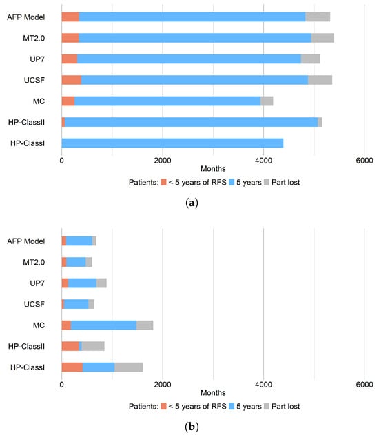
Figure 3.
Cumulative five-year RFS distribution (in months) among the cohort of patients (n = 100) with and without recurrence: (a) patients within criteria; (b) patients outside criteria. Each bar represents the total RFS time for each patient group. The orange segment indicates the number of RFS months for patients who relapsed within 60 months (5 years) post-transplant; the blue segment corresponds to those who remained relapse-free during the same period (patients who stayed in the Disease-Free state beyond 60 months); and the grey segment represents the time lost due to relapse—that is, the number of months (within the first five years after transplantation) that patients remained in the Recurrence state, assuming they did not die during the observation period.
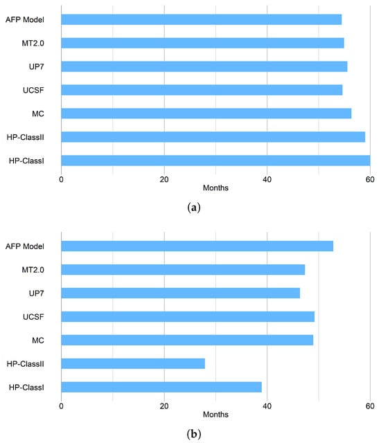
Figure 4.
Estimated five-year average RFS for: (a) Patients within criteria, and (b) Patients outside criteria.
Therefore, both HP classes maximise RFS for patients within the criteria, as they show the highest number of RFS months and the fewest months lost, with HP-ClassI being the most favourable. This conclusion is confirmed by analysing the average RFS for patients within the criteria (Figure 4a) where both HP classes exhibit the highest average RFS.
For patients outside the criteria (Figure 3b), both HP classes show the highest number of RFS months among patients who experienced recurrence (orange segment), while UCSF shows the lowest value. HP-ClassII has the fewest RFS months among patients who did not relapse (blue segment) and is the only criterion where the RFS months for relapsed patients exceed those for non-relapsed patients. Additionally, both HP classes record the highest number of RFS months lost among relapsed patients (grey segment). This indicates that both HP classes minimise RFS for patients outside the criteria.
When examining the average RFS for patients outside the criteria (Figure 4), both HP classes clearly differentiate themselves from the other criteria. They display the lowest average RFS among patients outside the criteria—particularly HP-Class II—and also exhibit the largest difference in average RFS between patients within and outside the criteria. In conclusion, both HP classes optimise RFS after transplantation.
For patients outside the criteria (Figure 3b), both HP classes show the highest number of RFS months among patients who experienced recurrence (orange segment), while UCSF presents the lowest value. HP-Class II has the fewest RFS months among patients who did not relapse (blue segment) and is the only criterion where the RFS months for relapsed patients exceed those for non-relapsed patients. Moreover, both HP classes record the greatest number of RFS months lost among relapsed patients (grey segment).
This suggests that both HP classes minimise RFS for patients outside the criteria because they tend to include more patients with a poor prognosis—those who relapsed within five years post-transplant. This outcome is, in fact, favourable: patients classified as outside the criteria are expected to have a higher likelihood of recurrence after transplantation. Therefore, in (Figure 3b), results for patients outside the criteria (b) are considered positive when the RFS bar is predominantly orange and grey, as this indicates a higher proportion of patients who actually relapsed, reflecting good predictive discrimination of the criteria.
3.2.2. Life Years Gained, LYG
Another relevant health outcome is life years gained, LYG. A summary of this measure for the different criteria under consideration is displayed in Figure 5.
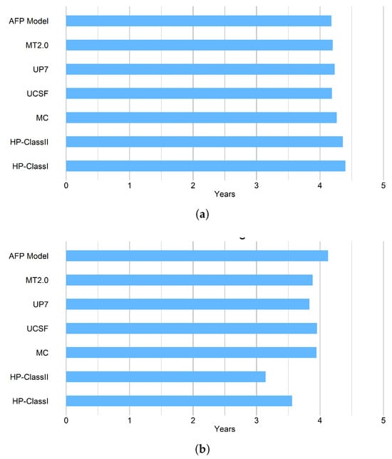
Figure 5.
Estimated five-year average life years gained per patient with HCC following liver transplantation for: (a) patients within criteria; (b) patients outside criteria.
For patients within the criteria (Figure 5a), HP-ClassI demonstrates the highest average LYG, providing an average of 0.19 additional LYG compared with the traditional criteria. HP-ClassII ranks second, with an average additional gain of 0.15 LYG. The remaining traditional criteria show comparable values for the average LYG. Similarly, for patients outside the criteria (Figure 5b), both HP classes display the lowest average LYG, with HP-Class II showing the lowest value. We can also observe that HP-ClassII is the only criterion for which the difference in average LYG between patients within and outside the criteria exceeds one year. Overall, HP-ClassII provides the largest improvement in post-transplant life expectancy, followed by HP-ClassI.
3.2.3. QALYs
After analysing the health benefits associated with each criterion in terms of RFS and LYG, it is now essential to compare the criteria with respect to their impact on the quality of life of LT patients, expressed in terms of QALYs. After all, extending survival has limited value if it is not accompanied by a corresponding improvement in quality of life. The comparison of different criteria for patients within the criteria in terms of QALYs is presented in Figure 6.
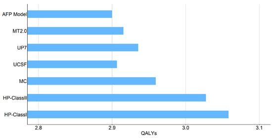
Figure 6.
Estimated five-year average quality-adjusted life years (QALYs) gained for a patient within the criteria.
For patients within the criteria (Figure 6), HP-Class I exhibits the highest quality of life, with an average of 3.06 QALYs, followed by HP-Class II with 3.03 QALYs. Compared with the traditional criteria, HP-Class I and HP-Class II show average increases of 0.13 and 0.10 QALYs, respectively. Among the traditional criteria, patients selected according to the AFP Model present the lowest average quality of life, with approximately 2.90 QALYs. Overall, patients classified by the HP criteria as having a good prognosis experience, on average, a higher quality of life.
3.2.4. Costs
An essential component of this analysis is the evaluation of the costs associated with each selection criterion. Although direct costs are exclusively attributed to HP, the long-term clinical effectiveness of each criterion influences the overall costs. This underscores the importance of performing a comprehensive cost analysis.
In this work, the cost-effectiveness analysis considers both five-year and annual costs, enabling comparison of clinical outcomes with financial expenditures and providing transparency regarding the economic impact of the selection criteria. Table 8 shows the estimated average annual costs per patient over five years for each criterion under consideration, along with the total costs for the five years. It is important to note that an annual discount rate of 3% was applied in the computation of these values, except for the initial case when , as discounting does not apply at baseline.
Table 8.
Estimated average annual and five-year total costs (in US$) per patient within each selection criterion.
Analysing the average total cost over five years (Table 8), patients selected by HP-ClassII incur the highest average total cost, while patients selected by MC have the lowest, with a difference of $2756.38, which is less than the initial cost of using HP ($7467.05). Patients selected by MC have the lowest costs to the healthcare system. On the other hand, in the yearly basis analysis, both HP classes are the least expensive during years one to four. In the fifth year, MC becomes the most expensive, while HPClassI is the least costly; in this year, however, costs among the criteria considered differ less than in previous years.
3.2.5. Cost-Effectiveness Analysis
We assessed the viability of the LT criteria under study from the perspective of the U.S. healthcare system. Two cost-effectiveness measures were considered: the Cost-Effectiveness Ratio (CER) and the Incremental Cost-Effectiveness Ratio (ICER). The CER corresponds to the ratio between total cost and total QALYs, representing the average cost per quality-adjusted life year gained. In contrast, the ICER quantifies whether one criterion is more cost-effective than another by expressing the additional cost required to gain one extra QALY. In this study, the ICER was computed relative to the MC, the most commonly used benchmark.
The main findings derived from the cost-effectiveness analysis are summarised in Figure 7 and Table 9.
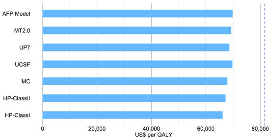
Figure 7.
Estimated five-year cost-effectiveness ratio (CER) for a patient within each criterion. The cost-effectiveness threshold (GDP per capita [47]) is indicated by the dashed dark blue line. HP classes correspond to HepatoPredict.AI version 3.
Table 9.
Estimated five-year averages of QALYs, costs, and ICER (relative to the Milan Criteria) for patients meeting the criterion.
Figure 7 shows that all CERs are below the U.S. GDP per capita [47] threshold, which indicates that the cost-effectiveness of using each criterion is acceptable and favourable by U.S. economic standards. HP-ClassI has the lowest CER, at approximately $64 735.43/QALY, making it the most cost-effective criterion. HP-ClassII follows as the second most cost-effective, with an CER of $65 825.03/QALY.
Figure 6 illustrates the nominal QALY values for each criterion under analysis, whereas Table 9 also presents the corresponding incremental ICER values. As shown in Table 9, UP7, UCSF, AFP Model, and MT2.0 have negative ICERs, indicating that MC dominates these criteria due to lower cost and higher QALY gains. In contrast, both HP classes are the only criteria that are cost-effective relative to MC, offering greater outcomes at higher costs, with ICERs below the U.S. GDP per capita ($81,632.25), consistent with WHO cost-effectiveness standards [35]. HP-ClassI has the lowest ICER ($14,689.58 per QALY), followed by HP-ClassII ($39,542.98 per QALY), $24,853.40 higher than HP-ClassI.
3.3. Deterministic Sensitivity Analysis
Since HP has emerged as the most cost-effective option based on the evaluated criteria, we conducted a univariate sensitivity analysis to assess whether its advantage is sustained within the U.S. context and whether it continues to outperform alternative criteria under varying parameter conditions. The primary objective is to determine whether, among eligible patients meeting each criterion, HP consistently remains the most cost-effective option across all scenarios.
For the one-way deterministic sensitivity analysis, we constructed a tornado diagram (Figure 8) to evaluate the influence of various input parameters, including probabilities, QALYs, and costs.
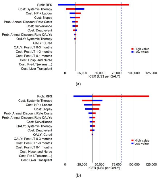
Figure 8.
Tornado diagrams illustrating the results of the one-way sensitivity analysis of the five-year ICER for (a) HP-Class I and (b) HP-Class II. Blue bars represent the lower bounds, whereas red bars represent the upper bounds of the input parameters. The cost-effectiveness threshold (GDP per capita) is shown as a dashed dark blue line, and the black vertical line denotes the ICER value from the base-case analysis.
For both HP classes, the five parameters with the greatest impact on the ICER are the probability of RFS, the cost of systemic therapy, the cost of the HP kit and associated hospital labour, the cost of biopsy, and the discount rate applied to costs and QALYs. The only parameter that causes both HP classes to exceed the cost-effectiveness threshold is an increase in the probability of RFS for HP and MC. For HP-Class I, it becomes dominant over MC when the probability of RFS is lower. The remaining parameters did not exhibit sufficient sensitivity to raise the ICER above the cost-effectiveness threshold, nor did they reveal any scenario in which the HP classes became simultaneously more effective and less costly than MC.
As the probability of RFS emerged as the parameter with the largest influence on cost-effectiveness, we conducted a sensitivity analysis varying its values within the corresponding lower and upper bounds. It is important to note that the probability of RFS differs across the criteria under study. Therefore, the variation in the ICER was calculated for all criteria. The results are presented in Table 10.
Table 10.
One-way sensitivity analysis of the five-year RFS parameter for all criteria: total costs, QALYs and ICER for patients meeting the criterion.
Regardless of changes in the probability of RFS, the UP7, UCSF, AFP Model, and MT2.0 criteria remain dominated by MC (Table 10). For both HP classes, higher values of this parameter yield a cost-benefit advantage over MC that exceeds the U.S. GDP per capita threshold ($81,632.25). Nonetheless, according to the World Health Organization (WHO), an ICER below three to five times a country’s GDP per capita remains economically acceptable, albeit relatively expensive [35]. At lower values of the RFS parameter, HP-Class I becomes dominant over MC, as the negative ICER indicates that HP-Class I provides greater benefits at a lower cost. Moreover, although HP-Class II is not dominant, it maintains a favourable ICER from the perspective of the U.S. healthcare system (Table 10).
4. Discussion
In this study, we compared HP with other criteria for selecting HCC patients for LT, highlighting differences in effectiveness, costs, and cost-effectiveness. Over a five-year horizon, both HP classes improved RFS and QALYs, providing a clinical advantage over criteria based solely on clinical variables and/or AFP levels. Importantly, HP integrates both clinical and molecular variables.
Following the RFS analysis, both HP classes improve RFS time after liver transplantation. Among patients within the criteria, HP-Class I provides the greatest maximisation of RFS time, while HP-Class II ranks second, with only a one-month difference between them. Among patients outside the criteria, HP-Class II exhibits the lowest RFS time and the largest gap between the average RFS times of patients within and outside the criteria. Contrary to expectations, HP-Class I does not minimise RFS for these patients, despite being the most effective in maximising RFS among those within the criteria. This is likely explained by its highly selective nature, as shown in Table 6, where it is identified as the second most restrictive criterion for patient inclusion. This finding may suggest that these criteria exclude potentially eligible patients with a good prognosis from receiving a transplant.
Another outcome analysed is patients’ life expectancy, assessed in terms of life years gained (LYG) over a five-year horizon, which decreases substantially among relapsed patients, whose five-year survival rate is only 38.82%. Although HP-Class II does not yield the highest values for patients within the criteria—HP-Class I performs slightly better—the difference between the two classes is minimal, corresponding to less than one month in mean LYG. The main advantage of the HP criteria lies in their ability to distinguish between patients with good and poor prognoses, as previously observed in the RFS analysis. The difference in LYG between patients within and outside the criteria is 0.84 years for HP-Class I and 1.22 years for HP-Class II, which is markedly higher than for the remaining criteria, where the differences do not exceed 0.4 years.
Compared to MC, QALY gains were 0.07 for HP-Class I and 0.10 for HP-Class II, corresponding to 24 and 35 additional days of perfect health, respectively. For context, the QALY difference between a patient with recurrence and one without is only 0.05 per year (18 days). These gains may help patients return to work more efficiently and for longer periods, positively impacting the economically active population. As more individuals re-enter the labour market, macroeconomic benefits may arise, including increased GDP and growth at both local and national levels. Employers may also benefit from reduced costs due to fewer workforce absences and lower staff turnover.
Although HP-Class II was more costly than other criteria, the additional RFS and QALY gains might justify the investment. Cost-effectiveness analyses from a U.S. healthcare perspective indicate that these superior clinical outcomes outweigh the higher costs. In the base case analysis, MC was 0.75% less expensive than HP-Class I (incremental cost: $1513.40) and 1.37% less expensive than HP-Class II (incremental cost: $2756.39), considering both pre- and post-transplant costs. Both HP classes were the only criteria found to be cost-effective relative to MC.
Compared to MC, the lowest-cost criterion, HP-Class II incurs an additional $2756.38, which is considerably less than the initial investment of $7467.05 for using HP. Over five years, HP has reduced post-transplant costs by improving long-term outcomes across all outcome metrics and lowering post-transplant expenditures. Costs are discounted annually, reducing the impact of future expenditures. The decrease in post-transplant costs is driven by both HP classes optimising RFS, selecting fewer patients with poor prognosis. This results in savings, as treatment costs for patients with recurrence are higher, and lower mortality further reduces costs associated with death.
The sensitivity analysis identified the probability of RFS as a critical parameter, with the most significant impact on the ICER. Fluctuations in this parameter lead to substantial changes in the ICER, which can influence conclusions. While variations in other parameters also affect the ICER, they do not alter the overall conclusions regarding cost-effectiveness.
This model has several limitations. First, the cohort used, while realistically reflecting the expected recurrence rate, was also employed to train the HP algorithm, which may have introduced bias. A fully independent cohort of 62 patients with a low recurrence rate (<15%) was tested, but due to its small size, it was not used for the primary analysis. Second, the availability of patient data in hospitals is limited, as transplant patients are generally selected using traditional criteria, resulting in the loss of information on patients who do not meet these criteria, which could be important for evaluating new tools. Finally, only HCC explant specimens were used, rather than biopsy samples, which would be the expected input for HP in practice. Further studies using HCC biopsy samples and an independent cohort are necessary to validate these findings.
Information on costs and QALYs is limited for most countries and, when available, is often derived from published studies that frequently omit essential details, such as the time frame of costs or the regional and perspective-specific context, making data collection and analysis more challenging.
Additionally, this model does not account for indirect or societal costs, such as lost productivity, transportation, or informal care provided by family and friends. Although these costs were not included, the ICER conclusions are likely robust, as such costs would similarly affect all patients, resulting in a proportional increase in total costs across criteria. Future economic evaluations should incorporate a social cost–effectiveness analysis.
The mortality probability for patients without relapse was derived from survival curves of all transplanted patients in the U.S., which included both patients with and without relapse. Although this represents a limitation, its impact is likely minimal given the low proportion of patients who develop relapse and the large sample size of 8066 patients. Additionally, Mazzaferro et al. [18] reported that HCC-related mortality is low relative to other causes among transplant patients.
Since this analysis focuses on patient follow-up over five years post-transplant, it does not account for the risks of complications or death during the biopsy, nor the probability of death during the transplant procedure. Future studies should address these risks to evaluate their potential impact.
Finally, there is a lack of comparable studies evaluating different criteria for selecting HCC patients for transplantation. This scarcity of literature limits the ability to compare our results with other data, making it difficult to generalise and externally validate the conclusions, particularly regarding QALYs, costs, and ICER metrics.
5. Conclusions
This study provides a comprehensive economic analysis of the clinical and economic implications of different patient selection criteria for patients with HCC undergoing LT. The results demonstrate that both HP classes offer greater benefits to the healthcare system and patient outcomes while supporting fairer organ allocation, making HP a promising tool to optimise resources and improve post-transplant outcomes. Both HP classes also present an acceptable cost-effective advantage over MC, particularly HP-Class II, justifying their implementation as a viable alternative.
Despite limitations, including data scarcity and the use of cohorts differing from the training set, this study represents the first analysis of its kind, and it makes an essential contribution by highlighting the need for further research with larger and more diverse patient populations to validate and strengthen these findings. Overall, the study offers new perspectives for optimising HCC patient selection for LT, improving organ allocation, promoting sustainability, and enhancing long-term outcomes through more efficient patient selection.
Author Contributions
Conceptualization, H.P., R.J.F. and H.M.; methodology, H.P., R.J.F. and H.M.; software, H.P.; validation, H.P., R.J.F. and H.M.; formal analysis, H.P., R.J.F. and H.M.; investigation, H.P.; data curation, H.P.; writing—original draft preparation, H.P.; writing—review and editing, H.P., R.J.F. and H.M.; visualization, H.P.; supervision, R.J.F. and H.M.; project administration, H.P., R.J.F. and H.M.; funding acquisition, R.J.F. and H.M. All authors have read and agreed to the published version of the manuscript.
Funding
This research was funded by Fundação para a Ciência e a Tecnologia (UID/00006/2023 and UID/04561/2025).
Data Availability Statement
Restrictions apply to the availability of these data. Data were obtained from Ophiomics and are available at https://www.ophiomics.com/ (accessed on 1 March 2024).
Acknowledgments
The authors gratefully acknowledge Ophiomics for providing access to the dataset used in this research to estimate recurrence-free survival (RFS).
Conflicts of Interest
The authors declare no conflicts of interest.
References
- Ferlay, J.; Ervik, M.; Lam, F.; Laversanne, M.; Colombet, M.; Mery, L.; Piñeros, M.; Znaor, A.; Soerjomataram, I.; Bray, F. Global Cancer Observatory: Cancer Today (Version 1.1); International Agency for Research on Cancer: Lyon, France, 2024; Available online: https://gco.iarc.who.int/today (accessed on 15 June 2024).
- Rumgay, H.; Ferlay, J.; de Martel, C.; Georges, D.; Ibrahim, A.S.; Zheng, R.; Wei, W.; Lemmens, V.E.; Soerjomataram, I. Global, regional and national burden of primary liver cancer by subtype. Eur. J. Cancer 2022, 161, 108–118. [Google Scholar] [CrossRef]
- Galle, P.R.; Forner, A.; Llovet, J.M.; Mazzaferro, V.; Piscaglia, F.; Raoul, J.L.; Schirmacher, P.; Vilgrain, V. EASL clinical practice guidelines: Management of hepatocellular carcinoma. J. Hepatol. 2018, 69, 182–236. [Google Scholar] [CrossRef]
- Rich, N.E.; Yopp, A.C.; Singal, A.G.; Murphy, C.C. Hepatocellular carcinoma incidence is decreasing among younger adults in the United States. Clin. Gastroenterol. Hepatol. 2020, 18, 242–248. [Google Scholar] [CrossRef]
- Rich, N.E.; Hester, C.; Odewole, M.; Murphy, C.C.; Parikh, N.D.; Marrero, J.A.; Yopp, A.C.; Singal, A.G. Racial and ethnic differences in presentation and outcomes of hepatocellular carcinoma. Clin. Gastroenterol. Hepatol. 2019, 17, 551–559. [Google Scholar] [CrossRef]
- World Health Organization. International Agency for Research on Cancer Cancer Today; World Health Organization: Geneva, Switzerland, 2016. [Google Scholar]
- Tsilimigras, D.I.; Aziz, H.; Pawlik, T.M. Critical analysis of the updated Barcelona clinic liver cancer (BCLC) group guidelines. Ann. Surg. Oncol. 2022, 29, 7231–7234. [Google Scholar] [CrossRef]
- Aksoy, S.O.; Unek, T.; Sevinc, A.I.; Arslan, B.; Sirin, H.; Derici, Z.S.; Ellidokuz, H.; Sagol, O.; Agalar, C.; Astarcioglu, I. Comparison of resection and liver transplant in treatment of hepatocellular carcinoma. Exp. Clin. Transpl. 2020, 18, 712–718. [Google Scholar] [CrossRef]
- Golabi, P.; Fazel, S.; Otgonsuren, M.; Sayiner, M.; Locklear, C.T.; Younossi, Z.M. Mortality assessment of patients with hepatocellular carcinoma according to underlying disease and treatment modalities. Medicine 2017, 96, e5904. [Google Scholar] [CrossRef]
- Llovet, J.; Kelley, R.; Villanueva, A.; Singal, A.; Pikarsky, E.; Roayaie, S.; Lencioni, R.; Koike, K.; Zucman-Rossi, J.; Finn, R. Hepatocellular Carcinoma Nat Rev Dis Primers. 7: 6. Article10 2021, 1038, 1038. [Google Scholar]
- Line, P.D. Selection criteria in liver transplantation for hepatocellular carcinoma: An ongoing evolution. BJS Open 2022, 6, zrac024. [Google Scholar] [CrossRef]
- Pinto-Marques, H.; Cardoso, J.; Silva, S.; Neto, J.L.; Goncalves-Reis, M.; Proenca, D.; Mesquita, M.; Manso, A.; Carapeta, S.; Sobral, M.; et al. A gene expression signature to select hepatocellular carcinoma patients for liver transplantation. Ann. Surg. 2022, 276, 868–874. [Google Scholar] [CrossRef]
- Llovet, J.M.; Pena, C.E.; Lathia, C.D.; Shan, M.; Meinhardt, G.; Bruix, J. Plasma biomarkers as predictors of outcome in patients with advanced hepatocellular carcinoma. Clin. Cancer Res. 2012, 18, 2290–2300. [Google Scholar] [CrossRef]
- Duvoux, C.; Roudot-Thoraval, F.; Decaens, T.; Pessione, F.; Badran, H.; Piardi, T.; Francoz, C.; Compagnon, P.; Vanlemmens, C.; Dumortier, J.; et al. Liver transplantation for hepatocellular carcinoma: A model including α-fetoprotein improves the performance of Milan criteria. Gastroenterology 2012, 143, 986–994. [Google Scholar] [CrossRef]
- Mazzaferro, V.; Regalia, E.; Doci, R.; Andreola, S.; Pulvirenti, A.; Bozzetti, F.; Montalto, F.; Ammatuna, M.; Morabito, A.; Gennari, L. Liver transplantation for the treatment of small hepatocellular carcinomas in patients with cirrhosis. New Engl. J. Med. 1996, 334, 693–700. [Google Scholar] [CrossRef]
- Yao, F.Y.; Ferrell, L.; Bass, N.M.; Watson, J.J.; Bacchetti, P.; Venook, A.; Ascher, N.L.; Roberts, J.P. Liver transplantation for hepatocellular carcinoma: Expansion of the tumor size limits does not adversely impact survival. Hepatology 2001, 33, 1394–1403. [Google Scholar] [CrossRef]
- Mazzaferro, V.; Llovet, J.M.; Miceli, R.; Bhoori, S.; Schiavo, M.; Mariani, L.; Camerini, T.; Roayaie, S.; Schwartz, M.E.; Grazi, G.L.; et al. Predicting survival after liver transplantation in patients with hepatocellular carcinoma beyond the Milan criteria: A retrospective, exploratory analysis. Lancet Oncol. 2009, 10, 35–43. [Google Scholar] [CrossRef]
- Mazzaferro, V.; Sposito, C.; Zhou, J.; Pinna, A.D.; De Carlis, L.; Fan, J.; Cescon, M.; Di Sandro, S.; Yi-Feng, H.; Lauterio, A.; et al. Metroticket 2.0 model for analysis of competing risks of death after liver transplantation for hepatocellular carcinoma. Gastroenterology 2018, 154, 128–139. [Google Scholar] [CrossRef]
- Ophiomics—Precision Medicine. Available online: https://www.ophiomics.com/ (accessed on 12 April 2025).
- Barton, P.; Bryan, S.; Robinson, S. Modelling in the economic evaluation of health care: Selecting the appropriate approach. J. Health Serv. Res. Policy 2004, 9, 110–118. [Google Scholar] [CrossRef] [PubMed]
- Sánchez-Périz, I.; Barrachina-Martínez, I.; Díaz-Carnicero, J.; Climent, A.M.; Vivas-Consuelo, D. Cost-Effectiveness Mathematical Model to Evaluate the Impact of Improved Cardiac Ablation Strategies for Atrial Fibrillation Treatment. Mathematics 2023, 11, 915. [Google Scholar] [CrossRef]
- Henderson, R.H.; Sampson, C.; Pouwels, X.G.; Harvard, S.; Handels, R.; Feenstra, T.; Bhandari, R.; Sepassi, A.; Arnold, R. Mapping the Landscape of Open Source Health Economic Models: A Systematic Database Review and Analysis: An ISPOR Special Interest Group Report. Value Health 2025, 28, 813–820. [Google Scholar] [CrossRef]
- Ross, A.; Kim, J.; McKay, M.; Pappas, E.; Hardaker, N.; Whalan, M.; Peek, K. The economics of a national anterior cruciate ligament injury prevention program for amateur football players: A Markov model analysis. Med. J. Aust. 2024, 221, 149–155. [Google Scholar] [CrossRef]
- Wu, W.; Tang, F.; Wang, Y.; Yang, W.; Zhao, Z.; Gao, Y.; Dong, H. Cost-effectiveness analysis of combination therapies involving novel agents for first/second-relapse patients with multiple myeloma: A Markov model approach with calibration techniques. Health Econ. Rev. 2025, 15, 21. [Google Scholar] [CrossRef]
- Wen, C.; Wang, X.; Shu, J.; Ruan, Y.; Xie, J.; Cheng, X.; Qi, B.; En, H.; Qin, G.; Huang, L.; et al. Estimated cost-effectiveness of early screening strategies for newborn hearing impairment using a Markov model. Front. Public Health 2025, 13, 1498860. [Google Scholar] [CrossRef]
- Worthington, J.; He, E.; Caruana, M.; Wade, S.; de Graaff, B.; Nguyen, A.L.T.; George, J.; Canfell, K.; Feletto, E. A Health Economic Evaluation of Routine Hepatocellular Carcinoma Surveillance for People with Compensated Cirrhosis to Support Australian Clinical Guidelines. MDM Policy Pract. 2025, 10, 23814683251344962. [Google Scholar] [CrossRef]
- Younossi, Z.M.; Paik, J.M.; Henry, L.; Pollock, R.F.; Stepanova, M.; Nader, F. Economic evaluation of non-invasive test pathways for high-risk metabolic dysfunction-associated steatotic liver disease (MASLD) in the United Kingdom (UK). Ann. Hepatol. 2025, 30, 101789. [Google Scholar] [CrossRef]
- Patel, M.V.; Davies, H.; Williams, A.O.; Bromilow, T.; Baker, H.; Mealing, S.; Holmes, H.; Anderson, N.; Ahmed, O. Transarterial therapies in patients with hepatocellular carcinoma eligible for transarterial embolization: A US cost-effectiveness analysis. J. Med. Econ. 2023, 26, 1061–1071. [Google Scholar] [CrossRef]
- Wu, X.; Kwong, A.; Heller, M.; Lokken, R.P.; Fidelman, N.; Mehta, N. Cost-effectiveness analysis of interventional liver-directed therapies for downstaging of HCC before liver transplant. Liver Transplant. 2024, 30, 151–159. [Google Scholar] [CrossRef] [PubMed]
- Rognoni, C.; Ciani, O.; Sommariva, S.; Bargellini, I.; Bhoori, S.; Cioni, R.; Facciorusso, A.; Golfieri, R.; Gramenzi, A.; Mazzaferro, V.; et al. Trans-arterial radioembolization for intermediate-advanced hepatocellular carcinoma: A budget impact analysis. BMC Cancer 2018, 18, 715. [Google Scholar] [CrossRef] [PubMed]
- Perelman, J.; Soares, M.; Mateus, C.; Duarte, A.; Faria, R.; Ferreira, L.; Saramago, P.; Veiga, P.; Furtado, C.; Caldeira, S.; et al. Methodological Guidelines for Economic Evaluation Studies of Health Technologies; INFARMED—National Authority of Medicines and Health Products, IP: Lisbon, Portugal, 2019. [Google Scholar]
- Qu, Z.; Krauth, C.; Amelung, V.E.; Kaltenborn, A.; Gwiasda, J.; Harries, L.; Beneke, J.; Schrem, H.; Liersch, S. Decision modelling for economic evaluation of liver transplantation. World J. Hepatol. 2018, 10, 837. [Google Scholar] [CrossRef] [PubMed]
- Sanders, G.D.; Neumann, P.J.; Basu, A.; Brock, D.W.; Feeny, D.; Krahn, M.; Kuntz, K.M.; Meltzer, D.O.; Owens, D.K.; Lisa, A. Prosser, L.A.; et al. Recommendations for Conduct, Methodological Practices, and Reporting of Cost-Effectiveness Analyses: Second Panel on Cost-Effectiveness in Health and Medicine. J. Am. Med. Assoc. 2016, 316, 1093–1103. [Google Scholar] [CrossRef]
- Chong, C.A.; Gulamhussein, A.; Heathcote, E.; Lilly, L.; Sherman, M.; Naglie, G.; Krahn, M. Health-state utilities and quality of life in hepatitis C patients. Am. J. Gastroenterol. 2003, 98, 630–638. [Google Scholar] [CrossRef]
- Bertram, M.Y.; Lauer, J.A.; De Joncheere, K.; Edejer, T.; Hutubessy, R.; Kieny, M.P.; Hill, S.R. Cost–effectiveness thresholds: Pros and cons. Bull. World Health Organ. 2016, 94, 925. [Google Scholar] [CrossRef] [PubMed]
- Rand, L.Z.; Melendez-Torres, G.J. Alternatives to the quality-adjusted life year: How well do they address common criticisms? Health Serv. Res. 2023, 58, 433–444. [Google Scholar] [CrossRef]
- Anchisi, M. Métodos Não Paramétricos Para Análise de Dados de Sobrevivência. Master’s Thesis, Faculdade de Ciências, Universidade de Lisboa, Lisboa, Portugal, 2011. [Google Scholar]
- Rocha, C.; Papoila, A.L. Análise de Sobrevivência; Sociedade Portuguesa de Estatística, SPE: Lisboa, Portugal, 2009; ISBN 978-972-8890-22-3. [Google Scholar]
- Kwong, A.J.; Kim, W.R.; Lake, J.R.; Schladt, D.P.; Schnellinger, E.M.; Gauntt, K.; McDermott, M.; Weiss, S.; Handarova, D.K.; Snyder, J.J.; et al. OPTN/SRTR 2022 annual data report: Liver. Am. J. Transplant. 2024, 24, S176–S265. [Google Scholar] [CrossRef]
- Maccali, C.; Chagas, A.L.; Boin, I.; Quiñonez, E.; Marciano, S.; Vilatobá, M.; Varón, A.; Anders, M.; Duque, S.H.; Lima, A.S.; et al. Recurrence of hepatocellular carcinoma after liver transplantation: Prognostic and predictive factors of survival in a Latin American cohort. Liver Int. 2021, 41, 851–862. [Google Scholar] [CrossRef]
- Roayaie, S.; Schwartz, J.D.; Sung, M.W.; Emre, S.H.; Miller, C.M.; Gondolesi, G.E.; Krieger, N.R.; Schwartz, M.E. Recurrence of hepatocellular carcinoma after liver transplant: Patterns and prognosis. Liver Transplant. 2004, 10, 534–540. [Google Scholar] [CrossRef]
- Pereira, H. Cost-Effectiveness Analysis of Selection Criteria for Liver Transplantation in Patients with Hepatocellular Carcinoma. Master’s Thesis, Faculdade de Ciências, Universidade de Lisboa, Lisboa, Portugal, 2025. [Google Scholar]
- U.S. Bureau of Labor Statistics. CPI Inflation Calculator. Available online: https://www.bls.gov/data/inflation_calculator.htm (accessed on 18 July 2024).
- Younossi, Z.M.; Teran, J.C.; Ganiats, T.G.; Carey, W.D. Ultrasound-Guided Liver Biopsy for Parenchymal Liver Disease (An Economic Analysis). Dig. Dis. Sci. 1998, 43, 46–50. [Google Scholar] [CrossRef]
- Cadier, B.; Bulsei, J.; Nahon, P.; Seror, O.; Laurent, A.; Rosa, I.; Layese, R.; Costentin, C.; Cagnot, C.; Durand-Zaleski, I.; et al. Early detection and curative treatment of hepatocellular carcinoma: A cost-effectiveness analysis in France and in the United States. Hepatology 2017, 65, 1237–1248. [Google Scholar] [CrossRef] [PubMed]
- Andrade, R.; Perez-Rojas, J.; da Silva, S.G.; Miskinyte, M.; Quaresma, M.C.; Frazão, L.P.; Peixoto, C.; Cubells, A.; Montalvá, E.M.; Figueiredo, A.; et al. HepatoPredict Accurately Selects Hepatocellular Carcinoma Patients for Liver Transplantation Regardless of Tumor Heterogeneity. Cancers 2025, 17, 500. [Google Scholar] [CrossRef] [PubMed]
- O’Neill, A. Gross Domestic Product (GDP) per Capita in the United States in Current Prices from 1987 to 2029. Available online: https://www.statista.com/statistics/263601/gross-domestic-product-gdp-per-capita-in-the-united-states/ (accessed on 18 July 2024).


Disclaimer/Publisher’s Note: The statements, opinions and data contained in all publications are solely those of the individual author(s) and contributor(s) and not of MDPI and/or the editor(s). MDPI and/or the editor(s) disclaim responsibility for any injury to people or property resulting from any ideas, methods, instructions or products referred to in the content. |
© 2025 by the authors. Licensee MDPI, Basel, Switzerland. This article is an open access article distributed under the terms and conditions of the Creative Commons Attribution (CC BY) license (https://creativecommons.org/licenses/by/4.0/).