Parallel Hypersurfaces in 𝔼⁴ and Their Applications to Rotational Hypersurfaces

Abstract

This study explores parallel hypersurfaces in four-dimensional Euclidean space ${\mathbb{E}}^4$, deriving explicit expressions for their Gaussian and mean curvatures in terms of the curvature functions of the base hypersurface. We identify conditions under which these parallel hypersurfaces are flat or minimal. The theory is applied to several key hypersurfaces, including rotational hypersurfaces, hyperspheres, catenoidal hypersurfaces, and helicoidal hypersurfaces, with detailed curvature computations and visualizations. These results not only extend classical curvature relations into higher-dimensional spaces but also offer valuable insights into curvature transformations, with practical applications in both theoretical and computational geometry.

1. Introduction

Surfaces constitute a fundamental object of study in differential geometry and have been thoroughly investigated by numerous authors [1,2]. Within this broad framework, a classical construction produces a parallel surface by offsetting a given surface along its unit normal field by a constant distance. This transformation provides a precise lens for tracking how curvature invariants behave under normal displacements. The origin of this notion is commonly traced to C. Dupin, who in the nineteenth century introduced families of surfaces sharing curvature properties [3]. Since then, the theory has expanded significantly—especially in the contexts of curvature evolutions and geometric modeling—and it extends naturally to higher dimensions, where we will consider parallel hypersurfaces in ${\mathbb{E}}^4$.

Numerous researchers have further developed this theory. For example, do Carmo’s work provides foundational results on curvature behavior and surface theory [4], while Gray investigates the structure of parallel surfaces and their singularities in higher dimensional spaces [5]. Several other contributions focus on classifying parallel surfaces, analyzing their minimality or flatness, and extending these constructions to ambient spaces of various dimensions [6,7]. These studies lay the groundwork for understanding geometric transformations driven by curvature in both low- and high-dimensional spaces. In some generalized models, if the normal vector is multiplied by a real-valued function depending on the principal curvatures, the resulting surface is referred to as a generalized focal surface [8,9].

A hypersurface, defined as a submanifold of codimension one in an ambient space, generalizes the notion of a surface to higher dimensions. In 4-dimensional Euclidean space ${\mathbb{E}}^4$, a hypersurface can be locally described by three parameters. The geometric study of such hypersurfaces involves understanding both their intrinsic properties and extrinsic behavior. There are notable studies that address curvature properties, classification, and special types of hypersurfaces in ${\mathbb{E}}^4$ [10,11,12,13]. Special classes of hypersurfaces in ${\mathbb{E}}^4$ —such as rotational hypersurfaces obtained by revolving curves around a plane [14], hyperspheres characterized by constant curvature [4], catenoidal hypersurfaces as higher-dimensional analogues of minimal catenoids [15], and helicoidal hypersurfaces generated by screw motions [16,17,18]—serve as canonical examples in differential geometry due to their symmetry and well-understood curvature properties.

The remainder of the paper is organized as follows. In Section 2, we provide the essential preliminaries on hypersurfaces in the four-dimensional Euclidean space ${\mathbb{E}}^4$, including the definitions of the first and the second fundamental forms, as well as the Gaussian curvature and the mean curvature. Section 3 introduces the concept of parallel hypersurfaces in ${\mathbb{E}}^4$ and presents our main theoretical results. Specifically, we derive explicit formulas for the principal curvatures, the Gaussian curvature, and the mean curvature of parallel hypersurfaces in terms of the curvature functions of the base hypersurface, and establish conditions under which these parallel hypersurfaces are flat or minimal. To demonstrate the applicability of our theoretical framework, Section 3 also includes detailed applications to several important classes of hypersurfaces: rotational hypersurfaces: rotational parameterization I (Section 3.1), rotational parameterization II (Section 3.1.1), hyperspheres (Section 3.1.2), catenoidal hypersurfaces (Section 3.1.3), and helicoidal hypersurfaces (Section 3.2). For each class, we compute the curvature properties of the associated parallel hypersurfaces and provide illustrative visualizations. Finally, Section 4 concludes the paper with a summary of our findings.

2. Preliminaries

In this section, we introduce the notation used throughout the paper and review the fundamental concepts related to surfaces. Let

$$x=\sum _{i=1}^4{x}_i{e}_i,\hspace{1em}y=\sum _{i=1}^4{y}_i{e}_i,\hspace{1em}z=\sum _{i=1}^4{z}_i{e}_i$$

be vectors in ${\mathbb{R}}^4$ endowed with the standard inner product

$$\langle x,y\rangle =x_1{y}_1+x_2{y}_2+x_3{y}_3+x_4{y}_4,$$

where $\{e_1,e_2,e_3,e_4\}$ is the canonical basis of ${\mathbb{R}}^4$. The norm of $x\in {\mathbb{R}}^4$ is $\parallel x\parallel =\sqrt{\langle x,x\rangle }$.

The (ternary) vector product of $x,y,z\in {\mathbb{R}}^4$ is defined by

$$x\otimes y\otimes z=\left|\begin{array}{cccc}{e}_1& e_2& e_3& e_4\\ x_1& x_2& x_3& x_4\\ y_1& y_2& y_3& y_4\\ z_1& z_2& z_3& z_4\end{array}\right|.$$

A hypersurface in ${\mathbb{E}}^4$ is a three-dimensional submanifold and can be locally represented by a smooth vector-valued function

$$\phi =\phi (r,s,t):U\subset {\mathbb{R}}^3\to {\mathbb{E}}^4,$$

(1)

where $r,s,t$ are real-valued parameters. The map $\phi$ defines a regular hypersurface if its partial derivatives with respect to these parameters are linearly independent at each point.

The tangent vectors of the hypersurface are given by

$${\phi }_r={\displaystyle \frac{\partial \phi }{\partial r}},\hspace{1em}{\phi }_s={\displaystyle \frac{\partial \phi }{\partial s}},\hspace{1em}{\phi }_t={\displaystyle \frac{\partial \phi }{\partial t}}.$$

These vectors span the tangent space at each point on the hypersurface. The unit normal vector $\mathcal{N}$ is defined as the unique vector perpendicular to all three tangent vectors, satisfying

$$\begin{array}{c}\hfill \langle \mathcal{N},{\phi }_r\rangle =0,\hspace{1em}\langle \mathcal{N},{\phi }_s\rangle =0,\hspace{1em}\langle \mathcal{N},{\phi }_t\rangle =0,\hspace{1em}\parallel \mathcal{N}\parallel =1.\end{array}$$

This vector can also be obtained using the generalized cross product

$$\mathcal{N}={\displaystyle \frac{{\phi }_r\times {\phi }_s\times {\phi }_t}{\parallel {\phi }_r\times {\phi }_s\times {\phi }_t\parallel }}$$

in ${\mathbb{E}}^4$ [9].

The coefficients of the first fundamental form of the hypersurface are defined by

$$g_{ij}=\langle {\phi }_i,{\phi }_j\rangle ,\hspace{1em}i,j\in \{r,s,t\},$$

(2)

which form the metric tensor $I=\left(g_{ij}\right)$.

The coefficients of the second fundamental form are expressed as

$$h_{ij}=\langle {\phi }_{ij},\mathcal{N}\rangle ,\hspace{1em}i,j\in \{r,s,t\},$$

(3)

which form the metric tensor $II=\left(h_{ij}\right)$. Thus, the matrices of the first fundamental form I and the second fundamental form $II$ are given by

$$I=\left[\begin{array}{ccc}{g}_{11}& g_{12}& g_{13}\\ g_{21}& g_{22}& g_{23}\\ g_{31}& g_{32}& g_{33}\end{array}\right]\hspace{1em}\mathrm{and}\hspace{1em}II=\left[\begin{array}{ccc}{h}_{11}& h_{12}& h_{13}\\ h_{21}& h_{22}& h_{23}\\ h_{31}& h_{32}& h_{33}\end{array}\right].$$

(4)

Using the first and second fundamental forms, the Gaussian curvature (Gauss-Kronecker curvature in higher dimensions) and the mean curvature are respectively given by

$$K={\displaystyle \frac{\det \left(II\right)}{\det \left(I\right)}}$$

(5)

and

$$H={\displaystyle \frac{1}{3}}\sum _{i,j}{g}^{ij}{h}_{ij},$$

(6)

where $\left(g^{ij}\right)$ is the inverse matrix of $\left(g_{ij}\right)$ [4,10].

3. Parallel Hypersurfaces in 𝔼⁴

This section introduces the concept of parallel hypersurfaces in ${\mathbb{E}}^4$ and summarizes their basic curvature relations.

Definition 1

([19]). Let $\mathcal{M}$ be a hypersurface given by the parametrization $\mathcal{M}:\phi (r,s,t)$. The parallel hypersurface ${\mathcal{M}}^{*}$ with the unit normal vector $\mathcal{N}(r,s,t)$ of $\mathcal{M}$ is parametrized as

$$\psi (r,s,t)=\phi (r,s,t)+\epsilon \mathcal{N}(r,s,t).$$

(7)

Theorem 1

([20]). Let ${\mathcal{M}}^{*}$ be the parallel hypersurface of the hypersurface $\mathcal{M}$ in ${\mathbb{E}}^n$. If $k_1,k_2,\dots ,k_{n-1}$ and $k_1^{*},k_2^{*},\dots ,k_{n-1}^{*}$ are the principal curvatures of $\mathcal{M}$ and ${\mathcal{M}}^{*}$ respectively, then

$$k_i^{*}={\displaystyle \frac{k_i}{1-\epsilon k_i}},\hspace{1em}i=1,\dots ,n-1.$$

As a direct consequence of Theorem 1, the following results for the four-dimensional Euclidean space are readily obtained.

Corollary 1.

If $\mathcal{M}$ and its parallel hypersurface ${\mathcal{M}}^{*}$ are given in ${\mathbb{E}}^4$, then the principal curvatures $k_1^{*},k_2^{*},k_3^{*}$, the Gaussian curvature $K^{*}$, and the mean curvature $H^{*}$ of the parallel hypersurface ${\mathcal{M}}^{*}$ are respectively given by

$$k_1^{*}={\displaystyle \frac{k_1}{1-\epsilon k_1}},\hspace{1em}{k}_2^{*}={\displaystyle \frac{k_2}{1-\epsilon k_2}},\hspace{1em}{k}_3^{*}={\displaystyle \frac{k_3}{1-\epsilon k_3}},$$

(8)

$$K^{*}={\displaystyle \frac{K}{1-3\epsilon H+{\epsilon }^2{K}_2-{\epsilon }^{3}K}},$$

and

$$H^{*}={\displaystyle \frac{3H-2\epsilon K_2+3{\epsilon }^{2}K}{3(1-3\epsilon H+{\epsilon }^2{K}_2-{\epsilon }^{2}K)}},$$

where $K_2=k_1{k}_2+k_1{k}_3+k_2{k}_3$ and H, K are the mean curvature and the Gaussian curvature of the base hypersurface $\mathcal{M}$, respectively.

Corollary 2. 

A parallel hypersurface is flat if only if the base hypersurface is flat.

Corollary 3. 

The parallel non-flat hypersurface ${\mathcal{M}}^{*}$ of $\mathcal{M}$ is minimal if and only if the distance ε is given by

$$\epsilon ={\displaystyle \frac{K_2\pm \sqrt{K_2^2-9KH}}{3K}}.$$

3.1. Parallel Hypersurface of Rotational Parameterization I

In this subsection, we evaluate a rotational hypersurface $\mathcal{M}$ in ${\mathbb{E}}^4$ with the parametrization

$$\phi (r,s,t)=\left(g\left(r\right)\cos s\cos t, g\left(r\right)\sin s\cos t, g\left(r\right)\sin t, h\left(r\right)\right).$$

(9)

The tangent vectors of $\mathcal{M}$ are

$$\begin{array}{ccc}\hfill {\phi }_r& =& \left(g^{\prime }\left(r\right)\cos s\cos t, g^{\prime }\left(r\right)\sin s\cos t, g^{\prime }\left(r\right)\sin t, h^{\prime }\left(r\right)\right),\hfill \\ \hfill {\phi }_s& =& \left(-g\left(r\right)\sin s\cos t, g\left(r\right)\cos s\cos t, 0, 0\right),\hfill \\ \hfill {\phi }_t& =& \left(-g\left(r\right)\cos s\sin t, -g\left(r\right)\sin s\sin t, g\left(r\right)\cos t, 0\right).\hfill \end{array}$$

The unit normal vector becomes

$$\mathcal{N}={\displaystyle \frac{1}{\sqrt{g^{\prime 2}+h^{\prime 2}}}}\left(h^{\prime }\cos s\cos t, h^{\prime }\sin s\cos t, h^{\prime }\sin t, -g^{\prime }\right).$$

(10)

The first fundamental form matrix of $\mathcal{M}$ and its inverse matrix are

$$I=\left[\begin{array}{ccc}{g}^{\prime 2}+h^{\prime 2}& 0& 0\\ 0& g^2{\cos }^{2}t& 0\\ 0& 0& g^2\end{array}\right]\hspace{1em}\Rightarrow \hspace{1em}{I}^{-1}=\left[\begin{array}{ccc}{\displaystyle \frac{1}{g^{\prime 2}+h^{\prime 2}}}& 0& 0\\ 0& {\displaystyle \frac{1}{g^2{\cos }^{2}t}}& 0\\ 0& 0& {\displaystyle \frac{1}{g^2}}\end{array}\right],$$

and the second fundamental form matrix is

$$II=\left[\begin{array}{ccc}{\displaystyle \frac{g^{″}{h}^{\prime }-h^{″}{g}^{\prime }}{g^{\prime 2}+h^{\prime 2}}}& 0& 0\\ 0& {\displaystyle \frac{-g^{\prime }{h}^{\prime }{\cos }^{2}t}{\sqrt{h^{\prime 2}+g^{\prime 2}}}}& 0\\ 0& 0& {\displaystyle \frac{-g^{\prime }{h}^{\prime }}{\sqrt{h^{\prime 2}+g^{\prime 2}}}}\end{array}\right].$$

Therefore, using $S=I^{-1}II$, we get the shape operator matrix as

$$\begin{array}{c}\hfill S=\left[\begin{array}{ccc}{\displaystyle \frac{g^{″}{h}^{\prime }-h^{″}{g}^{\prime }}{{(h^{\prime 2}+g^{\prime 2})}^{3/2}}}& 0& 0\\ 0& {\displaystyle \frac{-h^{\prime }}{g\sqrt{h^{\prime 2}+g^{\prime 2}}}}& 0\\ 0& 0& {\displaystyle \frac{-h^{\prime }}{g\sqrt{h^{\prime 2}+g^{\prime 2}}}}\end{array}\right].\end{array}$$

(11)

We obtain the Gaussian curvature K of $\mathcal{M}$ using $\det S$

$$K={\displaystyle \frac{h^{\prime 2}\left(g^{″}{h}^{\prime }-h^{″}{g}^{\prime }\right)}{g^2{(h^{\prime 2}+g^{\prime 2})}^{3/2}}},$$

and the mean curvature H of $\mathcal{M}$ using ${\displaystyle \frac{1}{3}}\mathrm{tr}\left(S\right)$ as

$$H={\displaystyle \frac{1}{3}}\left[{\displaystyle \frac{g^{″}{h}^{\prime }-h^{″}{g}^{\prime }}{{(h^{\prime 2}+g^{\prime 2})}^{3/2}}}-{\displaystyle \frac{2h^{\prime }}{g\sqrt{h^{\prime 2}+g^{\prime 2}}}}\right],$$

respectively.

Now, we turn our attention to the results regarding the parallel hypersurface of the relevant hypersurface. With the help of (7), we give the following theorem:

Theorem 2. 

Denote by ${\mathcal{M}}^{*}$ the parallel hypersurface of the rotational hypersurface given by the parametrization (9). Then, the parametrization of ${\mathcal{M}}^{*}$ is given by

$$\psi (r,s,t)=\left(g^{*}\left(r\right)\cos s\cos t, g^{*}\left(r\right)\sin s\cos t, g^{*}\left(r\right)\sin t, h^{*}\left(r\right)\right),$$

(12)

where

$$\begin{array}{c}\hfill g^{*}\left(r\right):=g\left(r\right)+{\displaystyle \frac{\epsilon h^{\prime }\left(r\right)}{\sqrt{g^{\prime }{\left(r\right)}^2+h^{\prime }{\left(r\right)}^2}}},\\ \hfill h^{*}\left(r\right):=h\left(r\right)-{\displaystyle \frac{\epsilon g^{\prime }\left(r\right)}{\sqrt{g^{\prime }{\left(r\right)}^2+h^{\prime }{\left(r\right)}^2}}}.\end{array}$$

Corollary 4. 

The parallel hypersurface ${\mathcal{M}}^{*}$ of a given rotational hypersurface $\mathcal{M}$ is another rotational hypersurface in ${\mathbb{E}}^4$.

Theorem 3. 

Consider the parallel hypersurface ${\mathcal{M}}^{*}$ given by the parametrization (12) of the rotational hypersurface $\mathcal{M}$ in ${\mathbb{E}}^4$. Then, the Gaussian curvature and mean curvature of ${\mathcal{M}}^{*}$ are respectively given by

$$K^{*}={\displaystyle \frac{h^{\prime 2}\left(g^{″}{h}^{\prime }-h^{″}{g}^{\prime }\right)}{\left[{(h^{\prime 2}+g^{\prime 2})}^{3/2}-\epsilon (g^{″}{h}^{\prime }-h^{″}{g}^{\prime })\right]{\left[g\sqrt{h^{\prime 2}+g^{\prime 2}}+\epsilon h^{\prime }\right]}^2}},$$

$$H^{*}={\displaystyle \frac{1}{3}}\left[{\displaystyle \frac{g^{″}{h}^{\prime }-h^{″}{g}^{\prime }}{{(h^{\prime 2}+g^{\prime 2})}^{3/2}-\epsilon (g^{″}{h}^{\prime }-h^{″}{g}^{\prime })}}-{\displaystyle \frac{2h^{\prime }}{g\sqrt{h^{\prime 2}+g^{\prime 2}}+\epsilon h^{\prime }}}\right].$$

Proof. 

Denote by ${\mathcal{M}}^{*}$ the parallel hypersurface given by Equation (12) of the rotational hypersurface $\mathcal{M}$. Then, from the shape operator matrix (11), the principle curvatures $k_1,k_2,$ and $k_3$ of $\mathcal{M}$ are

$$k_1={\displaystyle \frac{g^{″}{h}^{\prime }-h^{″}{g}^{\prime }}{{(h^{\prime 2}+g^{\prime 2})}^{3/2}}},\hspace{1em}{k}_2=k_3={\displaystyle \frac{-h^{\prime }}{g\sqrt{h^{\prime 2}+g^{\prime 2}}}}.$$

Using (8), we write the principle curvatures of ${\mathcal{M}}^{*}$ as

$$k_1^{*}={\displaystyle \frac{g^{″}{h}^{\prime }-h^{″}{g}^{\prime }}{{(h^{\prime 2}+g^{\prime 2})}^{3/2}+\epsilon (g^{″}{h}^{\prime }-h^{″}{g}^{\prime })}}, k_2^{*}=k_3^{*}={\displaystyle \frac{-h^{\prime }}{g\sqrt{h^{\prime 2}+g^{\prime 2}}-\epsilon h^{\prime }}} .$$

Since, $K^{*}=k_1^{*}{k}_2^{*}{k}_3^{*}$ and $H^{*}={\displaystyle \frac{1}{3}}\left(k_1^{*}+k_2^{*}+k_3^{*}\right)$, we obtain the result. □

Example 1. 

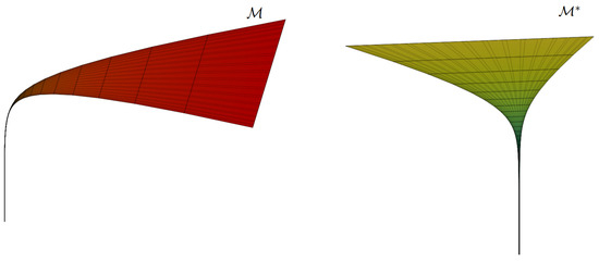
Consider the rotational hypersurface $\mathcal{M}$ given with (9) and its parallel hypersurface ${\mathcal{M}}^{*}$ given with (12), respectively. For $g\left(r\right)=e^r$, $h\left(r\right)=r$, and $\epsilon =1$, the rotational hypersurface and its parallel hypersurface have the following parametrizations:

$$\begin{array}{ccc}\hfill \phi (r,s,t)& =& \left(e^r\cos s\cos t, e^r\sin s\cos t, e^r\sin t, r\right),\hfill \end{array}$$

$$\psi (r,s,t)=\left(g^{*}\left(r\right)\cos s\cos t, g^{*}\left(r\right)\sin s\cos t, g^{*}\left(r\right)\sin t, h^{*}\left(r\right)\right),$$

where

$$\begin{array}{c}\hfill g^{*}\left(r\right):=e^r+{\displaystyle \frac{1}{\sqrt{e^{2r}+1}}},\\ \hfill h^{*}\left(r\right):=r-{\displaystyle \frac{1}{\sqrt{e^{2r}+1}}}.\end{array}$$

In this manuscript, all graphs of the projections of the hypersurfaces $\mathcal{M}$ and their parallel hypersurfaces ${\mathcal{M}}^{*}$ in Euclidean 3-space ${\mathbb{E}}^3$ are plotted using Julia (v1.12.1) with the GLMakie library (v0.13.6). The projection into three-dimensional space is carried out by eliminating the fourth component of the parametrization. One way to do this is by adding the third and fourth components and assigning their sum to the third coordinate in ${\mathbb{E}}^3$. Alternatively, depending on the chosen projection method, other combinations—such as adding the first and second components to form a new first coordinate—can also be considered. Additionally, fixing the parameter $t={\displaystyle \frac{\pi }{6}}$ selects a specific three-dimensional cross-section of the hypersurface (Figure 1).

3.1.1. Parallel Hypersurface of Rotational Parameterization II (In Case the Function $g\left(r\right)=r$)

If we take $g\left(r\right)=r$ in the parameterization (9), we reach another parameterization in ${\mathbb{E}}^4$:

$$\mathcal{M}:\phi \left(r,s,t\right)=\left(r\cos s\cos t,r\sin s\cos t,r\sin t,h\left(r\right)\right),$$

(13)

(see, [14]).

Substituting $g\left(r\right)=r$ in (10), the unit normal vector and the shape operator matrix become

$$\mathcal{N}={\displaystyle \frac{1}{\sqrt{1+h^{\prime 2}}}}\left(h^{\prime }\cos s\cos t, h^{\prime }\sin s\cos t, h^{\prime }\sin t, -1\right)$$

(14)

and

$$S=\left[\begin{array}{ccc}{\displaystyle \frac{-h^{″}}{{\left(1+h^{\prime 2}\right)}^{\frac{3}{2}}}}& 0\hspace{1em}& 0\\ 0& -{\displaystyle \frac{h^{\prime }}{r\sqrt{1+h^{\prime 2}}}}& 0\\ 0& 0& -{\displaystyle \frac{h^{\prime }}{r\sqrt{1+h^{\prime 2}}}}\end{array}\right],$$

(15)

respectively.

Let us now examine the results concerning the parallel hypersurface of the given hypersurface. By (7), we obtain the following theorem:

Theorem 4. 

Given that the hypersurface $\mathcal{M}$ is a rotational hypersurface with parametrization (13), the parallel hypersurface ${\mathcal{M}}^{*}$ of $\mathcal{M}$ is expressed by

$$\psi (r,s,t)=\left(\left(r+{\displaystyle \frac{\epsilon h^{\prime }}{\sqrt{1+h^{\prime 2}}}}\right)\cos s\cos t, \left(r+{\displaystyle \frac{\epsilon h^{\prime }}{\sqrt{1+h^{\prime 2}}}}\right)\sin s\cos t, \left(r+{\displaystyle \frac{\epsilon h^{\prime }}{\sqrt{1+h^{\prime 2}}}}\right)\sin t, h-{\displaystyle \frac{\epsilon }{\sqrt{1+h^{\prime 2}}}}\right).$$

(16)

Corollary 5. 

A parallel hypersurface of a rotational hypersurface is again a rotational hypersurface.

Theorem 5. 

Let ${\mathcal{M}}^{*}$ be a parallel hypersurface given with the parametrization (16) of rotational hypersurface $\mathcal{M}$ given with (13) in ${\mathbb{E}}^4.$ Then, the Gaussian curvature and the mean curvature of ${\mathcal{M}}^{*}$ are presented by

$$K^{*}={\displaystyle \frac{-h^{″}{h}^{\prime 2}}{\left[{\left(1+h^{\prime 2}\right)}^{\frac{3}{2}}+\epsilon h^{″}\right]{\left[r\sqrt{1+h^{\prime 2}}+\epsilon h^{\prime }\right]}^2}},$$

and

$$H^{*}=-{\displaystyle \frac{1}{3}}\left({\displaystyle \frac{h^{″}}{{\left(1+h^{\prime 2}\right)}^{\frac{3}{2}}+\epsilon h^{″}}}+{\displaystyle \frac{2h^{\prime }}{r\sqrt{1+h^{\prime 2}}+\epsilon h^{\prime }}}\right),$$

respectively.

Proof. 

Assume, ${\mathcal{M}}^{*}$ is the parallel hypersurface of the hypersurface defined through the equality (13). Then, from the shape operator matrix (15), the principle curvatures $k_1,k_2,$ and $k_3$ of $\mathcal{M}$ are

$$k_1={\displaystyle \frac{-h^{″}}{{\left(1+h^{\prime 2}\right)}^{\frac{3}{2}}}}, k_2=k_3=-{\displaystyle \frac{h^{\prime }}{r\sqrt{1+h^{\prime 2}}}}.$$

By (8), the principle curvatures of ${\mathcal{M}}^{*}$ are

$$k_1^{*}=-{\displaystyle \frac{h^{″}}{{\left(1+h^{\prime 2}\right)}^{\frac{3}{2}}+\epsilon h^{″}}}, k_2^{*}=k_3^{*}={\displaystyle \frac{-h^{\prime }}{r\sqrt{1+h^{\prime 2}}+\epsilon h^{\prime }}} .$$

Since, $K^{*}=k_1^{*}{k}_2^{*}{k}_3^{*}$ and $H^{*}={\displaystyle \frac{1}{3}}\left(k_1^{*}+k_2^{*}+k_3^{*}\right)$, we obtain the result. □

Example 2. 

Consider the rotational hypersurface $\mathcal{M}$ given with the parametrization (13) and its parallel hypersurface ${\mathcal{M}}^{*}$ given with (16), respectively (Figure 2). For $h\left(r\right)=\sqrt{3}r$ and $\epsilon =1$, the rotational hypersurface and its parallel hypersurface have the following parameterizations:

$$\begin{array}{ccc}\hfill \phi (r,s,t)& =& \left(r\cos s\cos t, r\sin s\cos t, r\sin t, \sqrt{3}r\right),\hfill \end{array}$$

$$\begin{array}{ccc}\hfill \psi (r,s,t)& =& \left(\left(r+{\displaystyle \frac{\sqrt{3}}{2}}\right)\cos s\cos t, \left(r+{\displaystyle \frac{\sqrt{3}}{2}}\right)\sin s\cos t, \left(r+{\displaystyle \frac{\sqrt{3}}{2}}\right)\sin t, \sqrt{3}r-{\displaystyle \frac{1}{2}}\right).\hfill \end{array}$$

3.1.2. Parallel Hypersurface of Hypersphere (In Case $g\left(r\right)=c\cos r$ and $h\left(r\right)=c\sin r$)

If we take $g\left(r\right)=c\cos r$ and $h\left(r\right)=c\sin r$ in the parametrization of the rotational hypersurface (9), a parametrization of a hypersphere becomes

$$\mathcal{M}:\phi (r,s,t)=\left(c\cos r\cos s\cos t, c\cos r\sin s\cos t, c\cos r\sin t, c\sin r\right).$$

(17)

Moreover, the unit normal vector field and the shape operator matrix yield

$$\mathcal{N}=\left(\cos r\cos s\cos t, \cos r\sin s\cos t, \cos r\sin t, \sin r\right)$$

and

$$\begin{array}{c}\hfill S=\left[\begin{array}{ccc}{\displaystyle \frac{-1}{c}}& 0& 0\\ 0& {\displaystyle \frac{-1}{c}}& 0\\ 0& 0& {\displaystyle \frac{-1}{c}}\end{array}\right],\end{array}$$

(18)

respectively.

Now, we write the parallel hypersurface of the hypersphere $\mathcal{M}$ by using the Equations (7) and (17).

Theorem 6. 

Let $\mathcal{M}$ be a hypersphere given with the parametrization (17) in ${\mathbb{E}}^4$. The parallel hypersurface ${\mathcal{M}}^{*}$ of $\mathcal{M}$ is given with the following parametrization:

$${\mathcal{M}}^{*}:\psi (r,s,t)=(c+\epsilon )\left(\cos r\cos s\cos t, \cos r\sin s\cos t, \cos r\sin t, \sin r\right).$$

(19)

Corollary 6. 

The parallel hypersurface ${\mathcal{M}}^{*}$ of a given hypersphere $\mathcal{M}$ is another hypersphere in ${\mathbb{E}}^4$.

Theorem 7. 

Let ${\mathcal{M}}^{*}$ be a parallel hypersurface with (19) of a given hypersphere $\mathcal{M}$ in ${\mathbb{E}}^4$. Then the Gaussian curvature and the mean curvature of ${\mathcal{M}}^{*}$ are

$$K^{*}={\displaystyle \frac{-1}{{(c+\epsilon )}^3}},\hspace{1em}{H}^{*}={\displaystyle \frac{-1}{(c+\epsilon )}},$$

respectively.

Proof. 

Denote by ${\mathcal{M}}^{*}$ the parallel hypersurface given by Equation (19) of the hypersphere $\mathcal{M}$. Then, from the shape operator matrix (18), the principle curvatures $k_1,k_2$, and $k_3$ of $\mathcal{M}$ are

$$k_1=k_2=k_3=-{\displaystyle \frac{1}{c}}.$$

From (8), the principle curvatures of ${\mathcal{M}}^{*}$ are

$$k_1^{*}=k_2^{*}=k_3^{*}=-{\displaystyle \frac{1}{c+\epsilon }}.$$

Since, $K^{*}=k_1^{*}{k}_2^{*}{k}_3^{*}$ and $H^{*}={\displaystyle \frac{1}{3}}\left(k_1^{*}+k_2^{*}+k_3^{*}\right),$ we obtain the result. □

Proposition 1. 

For the parallel hypersphere given by the expression (19), the ratio of the mean curvature to Gaussian curvature is

$${\displaystyle \frac{H^{*}}{K^{*}}}={(c+\epsilon )}^2.$$

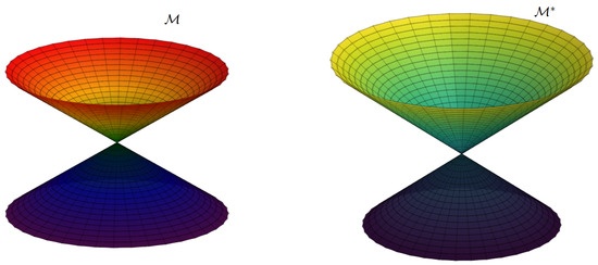
Example 3. 

Consider the hypersphere $\mathcal{M}$ given with the parametrization (17) and the parallel hypersurface ${\mathcal{M}}^{*}$ of $\mathcal{M}$ given with the parametrization (19), respectively (Figure 3). For $c=1$ and $\epsilon =1$, the hypersphere and its parallel hypersurface have the following parameterizations:

$$\begin{array}{ccc}\hfill \phi (r,s,t)& =& \left(\cos r\cos s\cos t, \cos r\sin s\cos t, \cos r\sin t, \sin r\right),\hfill \\ \hfill \psi (r,s,t)& =& \left(2\cos r\cos s\cos t, 2\cos r\sin s\cos t, 2\cos r\sin t, 2\sin r\right).\hfill \end{array}$$

3.1.3. Parallel Hypersurface of Catenoid Hypersurface (In Case $g\left(r\right)=\cosh r$, $h\left(r\right)=r$)

In the rotational hypersurface parameterization (9), if $g\left(r\right)=\cosh r$, $h\left(r\right)=r$ are taken, the catenoid hypersurface is presented by

$$\mathcal{M}:\phi (r,s,t)=\left(\cosh r\cos s\cos t, \cosh r\sin s\cos t, \cosh r\sin t, r\right).$$

(20)

The unit normal vector field and the shape operator matrix result in

$$\mathcal{N}={\displaystyle \frac{1}{\cosh r}}\left(\cos s\cos t, \sin s\cos t, \sin t, -\sinh r\right)$$

and

$$\begin{array}{c}\hfill S=\left[\begin{array}{ccc}{\displaystyle \frac{1}{{\cosh }^{2}r}}& 0& 0\\ 0& -{\displaystyle \frac{1}{{\cosh }^{2}r}}& 0\\ 0& 0& -{\displaystyle \frac{1}{{\cosh }^{2}r}}\end{array}\right],\end{array}$$

(21)

respectively.

We are now in a position to express the parametrization of the parallel hypersurface.

Theorem 8. 

Let $\mathcal{M}$ be a catenoid hypersurface given with the parametrization (20) in ${\mathbb{E}}^4$. The parallel hypersurface ${\mathcal{M}}^{*}$ of $\mathcal{M}$ is given with the following parametrization

$${\mathcal{M}}^{*}:\psi (r,s,t)=\left(g^{*}\left(r\right)\cos s\cos t, g^{*}\left(r\right)\sin s\cos t, g^{*}\left(r\right)\sin t, h^{*}\left(r\right)\right),$$

(22)

where

$$g^{*}\left(r\right):=\cosh r+{\displaystyle \frac{\epsilon }{\cosh r}},\hspace{1em}{h}^{*}\left(r\right):=r-{\displaystyle \frac{\epsilon \sinh r}{\cosh r}}.$$

Corollary 7. 

The parallel hypersurface ${\mathcal{M}}^{*}$ of a given catenoid hypersurface is not a catenoid hypersurface in ${\mathbb{E}}^4$.

Theorem 9. 

Let ${\mathcal{M}}^{*}$ be a parallel hypersurface with (22) of a given catenoid hypersurface $\mathcal{M}$ in ${\mathbb{E}}^4$. Then the Gaussian curvature and mean curvature of ${\mathcal{M}}^{*}$ are

$$K^{*}={\displaystyle \frac{1}{({\cosh }^{2}r-\epsilon )({\cosh }^{2}r+\epsilon )}},\hspace{1em}{H}^{*}={\displaystyle \frac{1}{3}}\left({\displaystyle \frac{1}{{\cosh }^{2}r-\epsilon }}-{\displaystyle \frac{2}{{\cosh }^{2}r+\epsilon }}\right),$$

respectively.

Proof. 

Denote by ${\mathcal{M}}^{*}$ the parallel hypersurface given by the Equation (22) of the hypersphere $\mathcal{M}$. Then, from the shape operator matrix (21), the principle curvatures $k_1,k_2$, and $k_3$ of $\mathcal{M}$ are

$$k_1={\displaystyle \frac{1}{{\cosh }^{2}r}}\hspace{1em}\mathrm{and}\hspace{1em}{k}_2=k_3=-{\displaystyle \frac{1}{{\cosh }^{2}r}}.$$

From (8), the principle curvatures of ${\mathcal{M}}^{*}$ are

$$k_1^{*}={\displaystyle \frac{1}{{\cosh }^{2}r-\epsilon }}\hspace{1em}\mathrm{and}\hspace{1em}{k}_2^{*}=k_3^{*}=-{\displaystyle \frac{1}{{\cosh }^{2}r+\epsilon }},$$

which completes the proof. □

Example 4. 

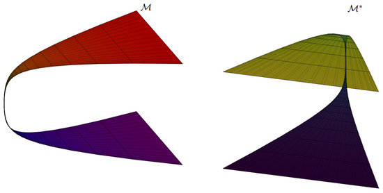
Consider the catenoid hypersurface $\mathcal{M}$ given with the parametrization (20) and the parallel hypersurface ${\mathcal{M}}^{*}$ of $\mathcal{M}$ given with the parametrization (22), respectively (Figure 4). For $\epsilon =-1$, parallel hypersurface of $\mathcal{M}$ has the following parameterization

$$\psi (r,s,t)=\left(\tanh r\sinh r\cos s\cos t,\tanh r\sinh r\sin s\cos t,\tanh r\sinh r\sin t, r+\tanh r\right).$$

3.2. Parallel Hypersurface of Helicoidal Hypersurface

The parametrization of helicoidal hypersurface in ${\mathbb{E}}^4$ is given as

$$\phi (r,s,t)=\left(r\cos s\cos t, r\sin s\cos t, r\sin t, f\left(r\right)+as+bt\right)$$

(23)

in [16].

The first partial derivatives of helicoidal hypersurface are

$$\begin{array}{ccc}\hfill {\phi }_r& =& (\cos s\cos t, \sin s\cos t, \sin t, f^{\prime })\hfill \\ \hfill {\phi }_s& =& (-r\sin s\cos t, r\cos s\cos t, 0, a)\hspace{1em}\hfill \\ \hfill {\phi }_t& =& (-r\cos s\sin t, -r\sin s\sin t, r\cos t, b).\hfill \end{array}$$

and the coefficients of the first fundamental form are

$$\begin{array}{ccc}\hfill g_{11}& =& 1+f^{\prime 2},\hfill \\ \hfill g_{12}& =& a{f}^{\prime },\hfill \\ \hfill g_{22}& =& r^2{\cos }^{2}t+a^2,\hfill \\ \hfill g_{13}& =& b{f}^{\prime },\hfill \\ \hfill g_{23}& =& ab,\hfill \\ \hfill g_{33}& =& r^2+b^2.\hfill \end{array}$$

(24)

We obtain the first fundamental form matrix of the hypersurface as

$$I=\left[\begin{array}{ccc}1+f^{\prime 2}& a{f}^{\prime }& b{f}^{\prime }\\ a{f}^{\prime }& r^2{\cos }^{2}t+a^2& ab\\ b{f}^{\prime }& ab& r^2+b^2\end{array}\right]$$

and

$$\det I=r^2(a^2+(b^2+(f^{\prime 2}+1)r^2){\cos }^{2}t).$$

(25)

We get the unit normal vector field of the helicoidal hypersurface as

$$\mathcal{N}={\displaystyle \frac{1}{\sqrt{\det I}}}\left(\begin{array}{c}r\left(\left(r{f}^{\prime }\cos t-b\sin t\right)\cos s\cos t-a\sin s\right),\\ r\left(\left(r{f}^{\prime }\cos t-b\sin t\right)\sin s\cos t+a\cos s\right),\\ r\left(r{f}^{\prime }\sin t+b\cos t\right)\cos t,\\ -r^2\cos t\end{array}\right).$$

(26)

The second partial derivatives of the helicoidal hypersurface are

$$\begin{array}{ccc}\hfill {\phi }_{rr}& =& (0, 0, 0, f^{″}),\hfill \\ \hfill {\phi }_{rs}& =& (-\sin s\cos t, \cos s\cos t, 0, 0)\hfill \\ \hfill {\phi }_{rt}& =& (-\cos s\sin t, -\sin s\sin t, \cos t, 0),\hfill \\ \hfill {\phi }_{ss}& =& (-r\cos s\cos t, -r\sin s\cos t, 0, 0),\hfill \\ \hfill {\phi }_{st}& =& (r\sin s\sin t, -r\cos s\sin t, 0, 0),\hfill \\ \hfill {\phi }_{tt}& =& (-r\cos s\cos t, -r\sin s\cos t, -r\sin t, 0).\hfill \end{array}$$

(27)

Using (26) and (27), we get the coefficients of the second fundamental form as

$$\begin{array}{ccc}\hfill h_{11}& =& -f^{″}{r}^2\cos t,\hfill \\ \hfill h_{12}& =& ar\cos t,\hfill \\ \hfill h_{22}& =& -r^2(r{f}^{\prime }\cos t-b\sin t){\cos }^{2}t,\hfill \\ \hfill h_{13}& =& br\cos t,\hfill \\ \hfill h_{23}& =& -a{r}^2\sin t,\hfill \\ \hfill h_{33}& =& -r^3(r{f}^{\prime }\cos t-b\sin t){\cos }^{2}t.\hfill \end{array}$$

(28)

The second fundamental form matrix is obtained as

$$II=\left[\begin{array}{ccc}-f^{″}{r}^2\cos t& ar\cos t& br\cos t\\ ar\cos t& -r^2(r{f}^{\prime }\cos t-b\sin t){\cos }^{2}t& -a{r}^2\sin t\\ br\cos t& -a{r}^2\sin t& -r^3(r{f}^{\prime }\cos t-b\sin t){\cos }^{2}t\end{array}\right],$$

and

$$\begin{array}{cc}\hfill \det II=& r^4\cos t[-\left(r{f}^{\prime }\cos t-b\sin t\right){\cos }^{3}t\left({\left(r{f}^{\prime }\cos t-b\sin t\right)}^2{r}^3{f}^{″}\cos t-a^{2}r-b^2\right)\hfill \\ \hfill \hspace{1em}& -a^2\sin t\left(2b\cos t-r^2{f}^{″}\sin t\right)].\hfill \end{array}$$

(29)

Theorem 10. 

Let $\mathcal{M}$ be a helicoidal hypersurface given with the parametrization (23) in ${\mathbb{E}}^4$. The Gaussian curvature of $\mathcal{M}$ is yielded as

$$K={\displaystyle \frac{\left[\begin{array}{c}-r^2\left(r{f}^{\prime }\cos t-b\sin t\right){\cos }^{4}t\left({\left(r{f}^{\prime }\cos t-b\sin t\right)}^2{f}^{″}\cos t-a^{2}r-b^2\right)\hfill \\ -a^2{r}^2\sin t\cos t\left(2b\cos t-r^2{f}^{″}\sin t\right)\hfill \end{array}\right]}{a^2+\left(b^2+(f^{\prime 2}+1)r^2\right){\cos }^{2}t}}.$$

Proof. 

Using the Equations (5), (25) and (29), the result is obtained. □

Theorem 11. 

Let $\mathcal{M}$ be a helicoidal hypersurface given with the parametrization (23) in ${\mathbb{E}}^4$. The mean curvature of $\mathcal{M}$ is yielded as

$$\begin{array}{c}\hfill H={\displaystyle \frac{1}{a^2+(r^2+b^2)co{s}^{2}t}}\left\{\begin{array}{c}(1+f^{\prime 2})\left((1+rco{s}^{2}t)(-r^3{f}^{\prime }co{s}^{3}t+r^{2}bsintco{s}^{2}t)\right)\hfill \\ -f^{″}{r}^{2}cost(a^2+(r^2+b^2)co{s}^{2}t)\hfill \\ +(a^2+b^{2}co{s}^{2}t)(-2f^{\prime }rcost+bsint)-f^{\prime }{b}^{2}rco{s}^{3}t\hfill \\ +a^{2}bsint-r^2{f}^{\prime }{a}^{2}co{s}^{3}t+r{a}^{2}bsintco{s}^{2}t.\hfill \end{array}\right.\end{array}$$

Proof. 

From the Equations (6), (24) and (28), the result is obtained. □

At this stage, having established the requisite geometric framework and analytical preliminaries, we are able to explicitly formulate the parametrization of the associated parallel hypersurface of a given helicoidal hypersurface $\mathcal{M}$.

Theorem 12. 

Let $\mathcal{M}$ be a helicoidal hypersurface given with the parametrization (23) in ${\mathbb{E}}^4$. The parallel hypersurface ${\mathcal{M}}^{*}$ of $\mathcal{M}$ is given with the following parametrization:

$$\psi (r,s,t)=\left(\begin{array}{c}r\cos s\cos t\left(1+\epsilon {\displaystyle \frac{r{f}^{\prime }\cos t-b\sin t}{\sqrt{\det I}}}\right)-\epsilon {\displaystyle \frac{a\sin s}{\sqrt{\det I}}},\\ r\sin s\cos t\left(1+\epsilon {\displaystyle \frac{r{f}^{\prime }\cos t-b\sin t}{\sqrt{\det I}}}\right)+\epsilon {\displaystyle \frac{a\cos s}{\sqrt{\det I}}},\\ r\sin t\left(1+\epsilon {\displaystyle \frac{r{f}^{\prime }\cos t}{\sqrt{\det I}}}\right)+\epsilon {\displaystyle \frac{b{\cos }^{2}t}{\sqrt{\det I}}},\\ f\left(r\right)+as+bt-\epsilon {\displaystyle \frac{r^2\cos t}{\sqrt{\det I}}}\end{array}\right),$$

(30)

where $\epsilon \in \mathbb{R}$.

Proof. 

Using the Equations (7) and (26), we get the result. □

Corollary 8. 

The parallel hypersurface ${\mathcal{M}}^{*}$ of a given helicoidal hypersurface is not a helicoidal hypersurface in ${\mathbb{E}}^4$.

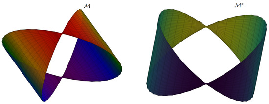
Example 5. 

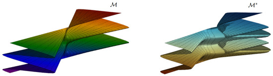
Consider the helicoidal hypersurface $\mathcal{M}$ given with the parametrization (23) and the parallel hypersurface ${\mathcal{M}}^{*}$ of $\mathcal{M}$ given with the parametrization (30), respectively (Figure 5). For $f\left(r\right)=r,a=1,b=2$, and $\epsilon =1$, the helicoidal hypersurface and the parallel hypersurface have the following parameterizations:

$$\begin{array}{ccc}\hfill \phi (r,s,t)& =& \left(r\cos s\cos t, r\sin s\cos t, r\sin t, r+s+2t\right),\hfill \\ \hfill \psi (r,s,t)& =& \left(\begin{array}{c}r\cos s\cos t\left(1+{\displaystyle \frac{r\cos t-2\sin t}{\sqrt{\det I}}}\right)-{\displaystyle \frac{\sin s}{\sqrt{\det I}}},\\ r\sin s\cos t\left(1+{\displaystyle \frac{r\cos t-2\sin t}{\sqrt{\det I}}}\right)+{\displaystyle \frac{\cos s}{\sqrt{\det I}}},\\ r\sin t\left(1+{\displaystyle \frac{r\cos t}{\sqrt{\det I}}}\right)+{\displaystyle \frac{2{\cos }^{2}t}{\sqrt{\det I}}},\\ r+s+2t-{\displaystyle \frac{r^2\cos t}{\sqrt{\det I}}}\end{array}\right).\hfill \end{array}$$

4. Conclusions

In this work, we investigated parallel hypersurfaces in the four-dimensional Euclidean space ${\mathbb{E}}^4$, deriving explicit expressions for their Gaussian and mean curvatures in terms of the curvature functions of the base hypersurface. We established conditions under which the parallel hypersurfaces are flat or minimal, thereby extending classical curvature relations to a higher-dimensional setting. The theoretical framework was illustrated through notable examples, including rotational hypersurfaces, hyperspheres, catenoidal hypersurfaces, and helicoidal hypersurfaces, for which the curvature properties of their associated parallel hypersurfaces were computed explicitly. Beyond offering concrete computational results, the study highlights how curvature-driven transformations behave in ${\mathbb{E}}^4$, paving the way for further analytical and applied investigations of special hypersurface geometries in both theoretical and computational contexts.

References

- Büyükkütük, S. Timelike factorable surfaces in Minkowski space-time. Sak. Univ. J. Sci. 2018, 22, 1939–1946. [Google Scholar] [CrossRef]
- Kişi, İ.; Öztürk, G.; Arslan, K. A new type of canal surface in Euclidean 4-space E4. Sak. Univ. J. Sci. 2019, 23, 801–809. [Google Scholar] [CrossRef][Green Version]
- Dupin, C. Applications de géOmétrie et de méCanique; Bachelier: Paris, France, 1822. [Google Scholar]
- do Carmo, M.P. Differential Geometry of Curves and Surfaces; Prentice Hall: Upper Saddle River, NJ, USA, 1976. [Google Scholar]
- Gray, A. Modern Differential Geometry of Curves and Surfaces with Mathematica; CRC Press: New York, NY, USA, 1998. [Google Scholar]
- Chen, B.Y.; Van der Veken, J. Complete classification of parallel surfaces in 4-dimensional Lorentzian space forms. Tohoku Math. J. 2009, 61, 1–40. [Google Scholar] [CrossRef]
- Pottmann, H.; Leopoldseder, S. A concept for parametric surface fitting which avoids the parametrization problem. Comput. Aided Geom. Des. 2003, 20, 343–362. [Google Scholar] [CrossRef]
- Nomizu, K.; Sasaki, T. Affine Differential Geometry; Cambridge University Press: New York, NY, USA, 1994. [Google Scholar]
- O Neill, B. Elementary Differential Geometry; Academic Press: Cambridge, MA, USA, 2006. [Google Scholar]
- Chen, B.Y. Geometry of Submanifolds; M. Dekker: New York, NY, USA, 1973. [Google Scholar]
- Gluck, H. Great circle fibrations and contact structures on the 3-sphere. Geom. Dedicata 2022, 216, 72. [Google Scholar] [CrossRef]
- Güler, E.; Kişi, Ö. Rotational hypersurfaces in S3(r) × ℝ product space. Sak. Univ. J. Sci. 2017, 21, 350–355. [Google Scholar] [CrossRef]
- Tosun, M.; Güngör, M.A.; Samancı, C.; Ersoy, S. Yarı-Öklidiyen uzayında yarı-hiperregle yüzeyler. Fırat Univ. J. Sci. Eng. 2004, 16, 597–606. [Google Scholar]
- Guler, E. Rotational Hypersurfaces Satisfying Δ′R = AR in the Four-Dimensional Euclidean Space. Politek. Derg. 2021, 24, 517–520. [Google Scholar] [CrossRef]
- Blair, D.E. On a generalization of the catenoid. Can. J. Math. 1975, 28, 231–236. [Google Scholar] [CrossRef]
- Güler, E.; Gümrük Karakoç, A. Dini-Type Helicodial Hypersurface in 4-Space. Ikonion J. Math. 2019, 1, 26–34. [Google Scholar]
- Yıldız, Ö.G.; Hızal, S.; Akyiğit, M. Type I+ helicoidal surfaces with prescribed weighted mean or Gaussian curvature in Minkowski space with density. Analele Stiintifice Ale Univ. Ovidius Constanta-Ser. Mat. 2018, 26, 99–108. [Google Scholar] [CrossRef]
- Yıldız, Ö.G.; Akyiğit, M. Constructions of type III+ helicoidal surfaces in Minkowski space with density. Int. Electron. J. Geom. 2019, 12, 20–25. [Google Scholar]
- do Carmo, M.P. Riemannian Geometry; Birkhäuser: Boston, MA, USA, 1992. [Google Scholar]
- Gorgulu, A. On the curvatures of the parallel hypersurfaces. Commun. Fac. Sci. Univ. Ank. Ser. A1 2003, 41, 85–91. [Google Scholar]
Disclaimer/Publisher’s Note: The statements, opinions and data contained in all publications are solely those of the individual author(s) and contributor(s) and not of MDPI and/or the editor(s). MDPI and/or the editor(s) disclaim responsibility for any injury to people or property resulting from any ideas, methods, instructions or products referred to in the content. |
© 2025 by the authors. Licensee MDPI, Basel, Switzerland. This article is an open access article distributed under the terms and conditions of the Creative Commons Attribution (CC BY) license (https://creativecommons.org/licenses/by/4.0/).