Abstract
This paper investigates a discrete-time compartmental model for computer virus propagation. The model classifies computers into susceptible, latent, and breaking-out states, with nonlinear dynamics driven by infection, recovery, and breakout processes. Stability is analyzed using the basic reproduction number , and chaotic behavior is demonstrated through phase portraits, bifurcation diagrams, and maximum Lyapunov exponents. To further characterize complexity, the complexity measure is computed, confirming the richness of the chaotic regime. In addition, control strategies are designed to stabilize the dynamics, and a master–slave synchronization scheme is proposed and validated. Numerical simulations highlight both the complexity and controllability of the system, underscoring its relevance for understanding and mitigating the propagation of computer viruses.
Keywords:
discrete-time model; computer virus; stability; chaos; MSC:
37N25; 37N35; 37D45; 34D20; 93D20; 93B52; 93C55
1. Introduction
Mathematical models serve as indispensable tools for unravelling the complexities of natural and engineered systems, offering a rigorous framework to simulate, predict, and ultimately understand intricate dynamic phenomena throughout diverse branches of science and engineering [1,2,3]. By abstracting real-world phenomena into equations, these models allow researchers to analyze system behavior, identify critical parameters, and forecast future states, providing insights that are often unattainable through purely empirical observations [4,5]. From climate prediction to financial markets and population dynamics, the application of mathematical modelling, leveraging tools such as differential and difference equations, has profoundly advanced our scientific understanding and decision-making capabilities [6].
Against this comprehensive backdrop, mathematical models have become indispensable tools in epidemiology to better comprehend and regulate epidemic outbreaks [7,8]. Foundational models like SIR and SIS frameworks have provided foundational insights into human disease dynamics, guiding public health interventions and policy formulations for decades [9,10]. Analogously, with the advent of pervasive digital connectivity, these epidemiological principles have been ingeniously adapted to comprehend the mechanisms behind the spread of computer viruses and other malicious software within networked environments [11,12]. The digital ecosystem presents unique challenges and characteristics that make it particularly amenable to modelling, allowing for the analysis of virus dissemination patterns, the effectiveness of countermeasures, and the identification of vulnerable network configurations [13].
While continuous-time differential equations have been widely employed in both classical epidemiology and early computer virus modelling [14,15], the inherent nature of computer networks often lends itself more naturally to a discrete-time framework [16,17]. The discrete-time framework is particularly suitable for modelling computer-virus propagation because updates, monitoring, and security interventions in networks occur at distinct, regular intervals, allowing the model to accurately capture event-driven dynamics that continuous-time approaches cannot directly represent. Network monitoring, software updates, firewall rule changes, and security patching cycles typically occur at distinct, regular intervals, representing discrete events rather than continuous flows [18]. Furthermore, the collection of data on infection rates and system states frequently happens in discrete snapshots [19], making difference equations a particularly well-suited tool for capturing these dynamics [20].
Moreover, several recent studies have also adopted discrete and fractional discrete frameworks to analyze and predict the spread of computer viruses. For example, Zhang et al. [16] introduced a delayed SLBS epidemic model to study the activation and transmission of latent computer viruses, providing deeper insights into the role of time delays in cyber-epidemics. Other scholars have investigated different discrete formulations of classical epidemic models, such as SIS, SIR, and SEIR structures, to better describe the propagation of malicious codes and worms across digital networks [21,22]. These works highlight that discrete approaches are not only mathematically tractable but also highly consistent with the packet-based operation of computer systems and network communication. Therefore, enriching traditional modeling with discrete and fractional operators has become an important direction in modern cyber-epidemic research. This discrete perspective provides a more realistic representation of how digital pathogens spread in environments characterized by periodic updates and event-driven responses, which is crucial in mitigating the persistent and escalating threat posed by computer viruses in our interconnected world [23,24].
Recognizing these practical realities, this paper introduces and thoroughly analyzes a discrete-time compartmental system specifically intended to simulate the spread of computer viruses. To clearly distinguish our contribution from the continuous-time formulation in [25], we emphasize that the discrete model adopted here captures event-driven processes such as packet exchanges, scheduled scans, downloads, and security updates, which occur at distinct time steps in real networks and cannot be directly represented within continuous-time dynamics. Moreover, the discrete system exhibits rich nonlinear phenomena, including bifurcations and chaotic attractors that were not reported in [25]. Finally, we design nonlinear control and master–slave synchronization schemes to suppress chaotic oscillations and stabilize the virus-free equilibrium, demonstrating both the theoretical novelty and the practical relevance of the proposed approach for cyber-defense. Our model classifies internal network components (computers) into three distinct states: Susceptible (S), representing uninfected and vulnerable machines; Latent (L), indicating computers that are infected but not yet actively spreading the virus; and Breaking-out (B), denoting machines that are actively transmitting the virus to other systems. The interactions and transitions between these states are governed by a set of nonlinear difference equations that encapsulate key factors such as the primary infection rate, recovery rates, the transition rate from latent to active spreading, and the influence of external network connectivity. This research aims to carry out a meticulous stability analysis of the model’s equilibrium states, with particular emphasis on the virus-free equilibrium. Its stability is critically evaluated through the computation of the basic reproduction number (). Beyond chaos detection, we also examine the system’s complexity using the complexity algorithm, which provides a complementary perspective to Lyapunov exponents in quantifying the unpredictability of the dynamics. This enables a more nuanced characterization of the transition between ordered and chaotic regimes. Moreover, recognizing the importance of maintaining network stability in the face of persistent viral threats, we design and test a nonlinear control strategy that successfully suppresses virus outbreaks by stabilizing the system around the virus-free equilibrium. In addition, we investigate synchronization phenomena between coupled discrete-time virus models, as synchronization control plays a crucial role in understanding and managing the dynamics of computer virus propagation. In interconnected networks, different subsystems or nodes may exhibit distinct infection patterns due to heterogeneous parameters or external perturbations. Synchronization aims to align the states of these subsystems, thereby enabling coordinated behavior and facilitating the design of efficient control strategies. Achieving synchronization in such models not only reveals the coupling effects between subnetworks but also provides a practical framework for suppressing chaotic oscillations and ensuring the stability of virus-free conditions across the entire network.
This work contributes to the growing research on computer-virus propagation models, with a particular focus on discrete-time frameworks. While previous studies have examined epidemic thresholds, bifurcations, and chaotic behavior in computer-virus dynamics, comprehensive analyses integrating nonlinear dynamics, complexity measures, and control/synchronization strategies within a single framework remain limited. The main objectives of this paper are: (i) to formulate a discrete-time SLB model capturing susceptible, latent, and breaking-out states within internal networks; (ii) to analyze the system’s stability and bifurcation properties, including computation of the basic reproduction number ; (iii) to quantify the complexity of chaotic regimes using spectral measures such as complexity; and (iv) to design and validate nonlinear control and synchronization schemes to mitigate outbreaks and stabilize the network. The key contributions include a detailed investigation of the rich nonlinear dynamics of the discrete-time SLB model, the demonstration of controllable chaos, and the development of practical cyber-defence strategies, which distinguish this work from prior literature. By linking stability analysis, chaos characterization through complexity, and nonlinear control/synchronization design, our framework provides a realistic and applicable tool for understanding and mitigating computer-virus propagation in networked environments. This integrated approach addresses the limitations of earlier discrete and continuous virus models and highlights the potential for coordinated cyber-defence strategies. Through these combined analyses, the proposed framework bridges equilibrium stability, bifurcation routes to chaos, quantitative complexity measures, and control/synchronization strategies, offering a comprehensive study of discrete-time computer virus propagation and contributing both to the theoretical foundation of discrete epidemic-like modelling and to practical cybersecurity applications.
What follows is presented in this order: Section 2 introduces the mathematical formulation of the proposed discrete-time compartmental model, including the analysis of its equilibrium points and the derivation of the basic reproduction number . The stability of the virus-free equilibrium is examined in Section 3 while Section 4 investigates the system’s nonlinear dynamics through bifurcation charts, Lyapunov exponents, and phase portraits. Section 5 presents the complexity analysis. Section 6 introduces a nonlinear control strategy and explores synchronization between coupled systems. Final remarks and prospective research extensions are addressed in Section 7.
2. The Discrete-Time SLB System
This section presents a discrete-time framework for simulating the propagation of a computer virus. We then focus on identifying the equilibrium points and calculating the basic reproduction number, as these are crucial for understanding the stability and spread dynamics of computer virus systems.
2.1. Description of the Model and Its Equilibrium Points
The model is inspired and adapted from previous work [25] to capture the dynamics of internal network behavior. For this model, we consider only internal computers that are currently connected to the internet, while external systems are excluded from the dynamics.
The internal computer population is divided into three distinct compartments:
- : the proportion of computers that are virus-free,
- : the proportion of computers that are infected but not yet actively spreading the virus (latent),
- : the proportion of computers that are actively breaking out and transmitting the virus.
At any given time t, these three proportions satisfy the constraint .
The continuous-time model that captures the interactions between susceptible, latent, and breaking-out computers is dictated by:
Equation (1) represents the classical continuous-time SLB model, which describes the spread of computer viruses in a closed internal network. The parameter denotes the external connection or input rate of new susceptible computers to the network. The infection rate quantifies how efficiently susceptible computers become infected through interaction with latent or breaking-out computers. The parameter is the breakout rate that governs the transition from the latent to the active spreading state. The recovery rates and correspond to the rates at which latent and breaking-out computers return to the susceptible state, respectively. All parameters are positive and reflect the main processes affecting virus transmission, recovery, and connectivity.
The SLB model focuses on the essential dynamics of virus propagation in internal networks, using susceptible (S), latent (L), and breaking-out (B) states. Other compartments, such as recovered/removed (R) or quarantined (Q), are excluded because cleaned computers can immediately return to the susceptible state, and isolation strategies are beyond the scope of the current study. Hence, the S-L-B dynamics adequately capture the virus propagation scenario considered here.
However, in practical applications, data on virus propagation is typically collected at discrete time intervals. Thus, a discrete-time model is more appropriate for simulating and analyzing the transmission of computer viruses. Accordingly, we obtain the following discrete-time version of the model:
The nonlinear dynamics of the discrete-time SLB model arise from the interactions between susceptible, latent, and breaking-out computers. The infection term represents the rate at which susceptible computers become infected through contact with latent or actively spreading computers. The recovery terms and and the breakout term further modulate the transitions between compartments in a state-dependent manner. These nonlinear terms drive the complex behaviors observed in the system, including bifurcations and chaos, and make the model fully reproducible and interpretable.
By considering a unit time step (), this choice is not arbitrary. In real cybersecurity monitoring, network states are typically recorded at discrete intervals, such as per scan cycle, per communication round, or per day. Therefore, setting corresponds to a normalized sampling period at which the system states are updated. This ensures that the discrete model remains physically interpretable and consistent with the practical way virus activity is measured, without introducing artificial chaotic effects. System (2) can be rewritten in the general recursive form:
where
This recursive formulation defines the system via an explicit update rule. Since each state relies uniquely on the preceding state , the solution’s existence and uniqueness are guaranteed for any given initial condition . Therefore, the solution sequence exists and is unique.
Finding the equilibrium states is essential for analyzing the dynamics of model (2), which requires solving the following equation:
We identify as an equilibrium point for the given equation. As this point signifies the absence of the malware, it is termed the virus-free equilibrium, and its properties will be thoroughly examined in upcoming discussions.
From the premise that , we derive:
Referred to as the viral equilibrium point , this solution describes a scenario where the virus remains present within the system. Its stability is generally investigated using numerical methods.
2.2. Basic Reproduction Number
The analysis focuses on the basic reproduction number , a threshold parameter that determines the stability of the virus-free equilibrium. Following the approach in [13], denotes the average number of secondary infections arising from a single infected computer before recovery or removal. Its computation is based on the compartments contributing to new infections, corresponding to the last two equations of system (2). Specifically, is given by the spectral radius of the next-generation matrix , where F and V are the Jacobian matrices of the new infection terms and transition terms , evaluated at the virus-free equilibrium.
The significance of in the context of computer-virus propagation is as follows:
- If , each infected computer generates, on average, less than one new infection, and the virus-free equilibrium is locally asymptotically stable. In this case, any infection introduced into the network will eventually die out.
- If , each infected computer produces more than one secondary infection on average, leading to potential outbreak and persistence of the virus within the network. This condition may also give rise to complex dynamics, including oscillations or chaotic behavior, depending on system parameters.
Thus, serves both as a theoretical tool to assess the risk of viral spread and as a practical guideline for designing effective control strategies, such as recovery interventions, synchronization-based containment, or other network security measures.
The Jacobian matrices are:
Then the next generation matrix is:
thus
3. Stability Evaluation of the Virus-Free Equilibrium
Within this section, we investigate the stability of the virus-free equilibrium point. The following theorem has a decisive role in the stability analysis of discrete dynamical systems:
Theorem 1
([26]). System (3) achieves asymptotic stability if and only if the eigenvalues of the Jacobian matrix J, determined at the fixed point, satisfy
Based on this result, we derive:
Theorem 2.
Suppose that and the following two conditions hold:
where
hence, the virus-free equilibrium of System (2) is locally asymptotically stable.
Proof.
By simple calculation, we obtain the Jacobian matrix
The corresponding characteristic equation:
The first eigenvalue of is because all parameters are positives, (), then we get:
hence, satisfies the stability condition stated in Theorem 1. For the polynomial
If , then . Indeed, since all parameters and , this follows directly from their definitions that
and
Moreover, the extra positive fractions in the expression for A ensure that , we get:
(from the Condition (10)).
Thus, , hence, the roots are complex conjugates. We denote them by and ,
under the conditions of the model , we have , so
which implies
Hence, all eigenvalues derived from the characteristic equation of the Jacobian matrix satisfy the conditions stated in Theorem 1. Consequently, is locally asymptotically stable. □
To explore the dynamic evolution of the proposed system, we perform numerical simulations using specific initial conditions and parameter values from [27] applied to System (2). The initial population distribution is:
And the parameters are set to:
These parameter values were chosen based on reported ranges in previous studies [27] to reflect realistic scenarios for internal network virus propagation. While exact real-world data are often unavailable due to confidentiality, these choices allow us to explore the typical dynamics of the system, including the rise of latent and breaking-out populations, as well as the efficacy of control strategies in stabilizing the virus-free state.
Using these values, we generate the simulation results presented in Figure 1 to study the essential dynamical features of the model. The simulation depicts a scenario where the computer virus is actively spreading within the network, resulting in a reduction in the virus-free population and an increase in both latent and active populations. The trends suggest that, over 100 months, the system has not yet reached an equilibrium or a peak in infection, particularly for the latent and breaking-out categories. The gradual nature of the changes indicates a relatively slow progression of the epidemic over this time frame.
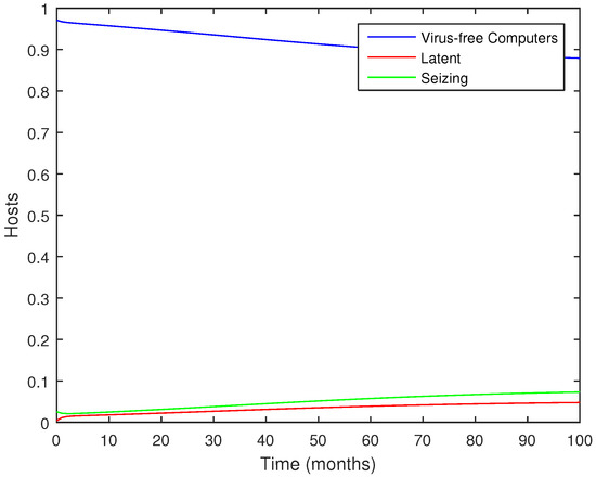
Figure 1.
Numerical results for the discrete model (2).
The stability analysis in this work focuses on the local behavior of the virus–free equilibrium using the basic reproduction number . Numerical simulations show that when , all trajectories initiated from different initial conditions converge to the virus–free state, suggesting that the equilibrium may also be globally stable. However, a complete analytical proof of global stability is mathematically demanding for discrete nonlinear systems and will be explored in future research. In contrast, when , the system undergoes a sequence of qualitative transitions, including periodic oscillations and period–doubling bifurcations leading to chaos. This confirms that parameter variations can trigger rich nonlinear behavior beyond local instability.
4. Bifurcation Dynamics and Chaotic Features
This section provides a detailed study of the discrete-time SLB system of computer viruses under three distinct parameter scenarios. The dynamical behavior is examined with respect to two critical parameters: the transition rate from latent to breaking-out computers () and the recovery rate of actively infected computers (). By varying these parameters, we investigate the dynamical transitions that carry the model from stability to chaos, using phase portraits, bifurcation diagrams, and MLE to capture the full spectrum of system dynamics.
In the first case, start from and take , we analyze how the system responds to variations in the transition rate over the interval . As shown in Figure 2, the bifurcation diagrams for the susceptible (S), latent (L), and breaking-out (B) classes reveal a clear evolution from stable fixed points to increasingly irregular and oscillatory behavior. Initially, all state variables demonstrate regular and periodic patterns. However, as , the rate at which latent computers break out increases, the dynamics grow more complex for S, L, and B, which develops a period-doubling structure leading to chaos. This behavior reflects how a high rate of transition from latency to active infection can destabilize the system and promote widespread outbreaks. The MLE plot (Figure 2d) provides quantitative support for these observations.
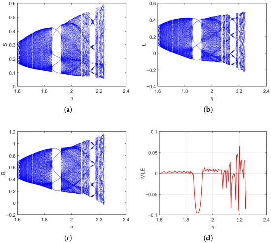
Figure 2.
Bifurcation and MLE of the discrete-time SLB model of computer viruses (2) as varies for = 2.1, = 0.1, = 0.5, . (a–c) Bifurcation of S, L, and B, (d) Maximum Lyapunov exponent (MLE).
All numerical results were obtained using MATLAB R2023a. The maximum Lyapunov exponent was calculated using the Jacobian matrix algorithm of Wu and Baleanu [28]. At each iteration, the Jacobian of the system was evaluated along the trajectory, and the Lyapunov index was estimated through QR-orthonormalization of tangent vectors. This standard procedure ensures accurate detection of chaotic behavior. To ensure reliability, bifurcation diagrams and MLE values were computed using long trajectories as shown in Figure 2. The small irregular oscillations in the MLE curve correspond to transitions between periodic windows and chaotic bands, which is a known property of discrete nonlinear systems. It stays negative for lower values, indicating stable dynamics, but becomes positive, confirming chaotic behavior. As latent computers convert more quickly to active infections, small differences in initial conditions amplify over time, making the system highly unpredictable.
Phase portraits across different settings of are shown in Figure 3. Fixing and using the same initial conditions and parameter values as in the previous simulations, a similar pattern is observed when varying the cure rate , as illustrated by the bifurcation diagram and MLE in Figure 4. As increases from 0.3 to 0.8, the system experiences instability and eventually chaotic oscillations, particularly in L and B. A moderate cure rate seems to destabilize the infection cycle, possibly due to feedback delays between infection and recovery. The MLE reflects this by becoming positive in intermediate values of , highlighting the nonlinear role of curing dynamics. Bifurcation diagrams were generated with fine parameter increments to ensure a robust representation of the system dynamics. Phase portraits for different values of are presented in Figure 5, further illustrating this transition. For low and , the system traces closed or spiral-like orbits, indicating periodic behavior. At higher values, the trajectories fragment and fill portions of the phase space, consistent with chaotic attractors. Case 1 demonstrates a progressive destabilization process, where increasing transition and cure rates can trigger chaos via period-doubling.
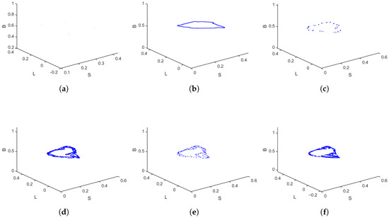
Figure 3.
Phase portraits of the discrete-time SLB model for , across different settings of ; (a) , (b) , (c) , (d) , (e) , (f) .
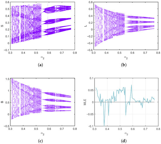
Figure 4.
Bifurcation and MLE of the discrete-time SLB model of computer viruses (2) as varies for . (a–c) Bifurcation of S, L, and B, (d) Maximum Lyapunov exponent (MLE).
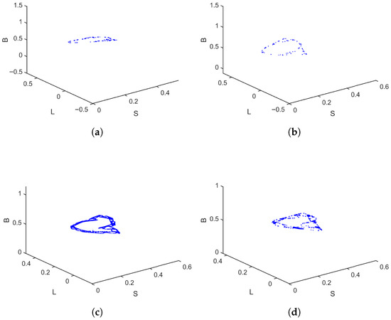
Figure 5.
Phase portraits of the discrete-time SLB model for , for different values of ; (a) , (b) , (c) , (d) .
In the second case, a different parameter setting is used , with now ranging from to . The bifurcation diagrams in Figure 6 reveal more abrupt and complex changes compared to the first case. The infected population B displays sudden bifurcations and dense oscillations as increases, and the latent class L exhibits irregular patterns even in the lower half of the range. This suggests that in certain configurations, even moderate increases in the rate of transition from latency to active infection can lead to dramatic destabilization. The MLE plot in Figure 6d shows narrow windows of positive values, indicating short-lived chaotic intervals. This intermittent chaos is often harder to detect but may result in unpredictable outbreaks or sudden bursts in virus activity. From a practical standpoint, this implies that even a brief increase in the infection activation rate can compromise the entire network’s stability. Phase portraits of the system for different values are shown in Figure 7. These portraits confirm the sensitivity of the system to , with trajectories becoming more irregular and fragmented as increases. Fixing and varying from 0.2 to 0.8, the bifurcation diagrams and MLE in Figure 8 reveal even sharper and more discontinuous transitions than in the first case. The breaking-out class B becomes extremely sensitive to the cure rate, with oscillations and chaotic windows appearing frequently. Phase portraits in Figure 9 further illustrate this high sensitivity. The attractors are irregular and fragmented, with less structure and higher density in the phase space. System trajectories show erratic and non-repeating behavior, a hallmark of chaos. This case highlights that under certain parameter combinations, the system becomes far more reactive to small parameter changes, leading to abrupt and significant chaotic behavior.
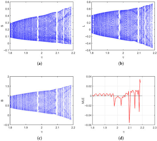
Figure 6.
Bifurcation and MLE of the discrete-time SLB model of computer viruses (2) as varies for . (a–c) Bifurcation of S, L, and B, (d) Maximum Lyapunov exponent (MLE).

Figure 7.
Phase portraits of the discrete-time SLB model (2) for , for different values: (a) , (b) , and (c) .
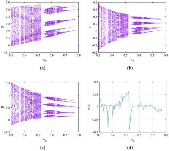
Figure 8.
Bifurcation and MLE of the discrete-time SLB model of computer viruses (2) as varies for . (a–c) Bifurcation of S, L, and B, (d) Maximum Lyapunov exponent (MLE).
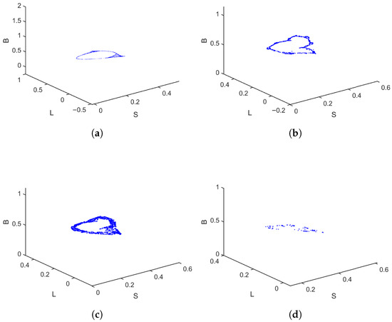
Figure 9.
Phase portraits of the discrete-time SLB system (2) for , for different values: (a) , (b) , (c) , and (d) .
Take the parameters . As shown in Figure 10, when varies from to , the bifurcation diagrams and MLE provide a clear depiction of the system’s dynamic behavior, particularly its transition to chaos. The system exhibits a classical period-doubling cascade into chaos with rising , as revealed by the bifurcation diagrams. The system’s stable fixed point undergoes successive bifurcations, leading to periodic oscillations of increasingly doubled periods (period-2, period-4). This cascade culminates in a broad, dense region, signaling the onset of chaotic dynamics marked by a strong dependence on initial conditions and unpredictable, non-repeating trajectories. Supporting this visual evidence, the MLE in Figure 10d quantitatively corroborates the system’s dynamics, being notably positive in the parameter ranges where the bifurcation diagrams indicate chaos. The MLE plot also highlights windows of periodicity within the chaotic band (approximately to ), where it temporarily drops to negative values, signifying stable periodic behavior. Phase portraits for different values are presented in Figure 11, further illustrating the system’s behavior across the parameter range. Similarly, when varying the cure rate for , the bifurcation diagrams and MLE in Figure 12 show that even as the cure rate of breaking-out computers increases from 0 to , the MLE remains positive across most values, with brief negative intervals suggesting short periods of relative stability or regular oscillations. Phase portraits for different values are shown in Figure 13, confirming these dynamics. Most trajectories show irregular, chaotic patterns, while certain parameter values corresponding to the negative MLE intervals display more structured, closed, or spiral orbits indicative of periodic or quasi-periodic behavior. Overall, this case demonstrates a system that predominantly behaves chaotically but exhibits intermittent windows of stability, highlighting the importance of carefully tuning parameters and to avoid unpredictable outbreaks and maintain control over virus propagation.
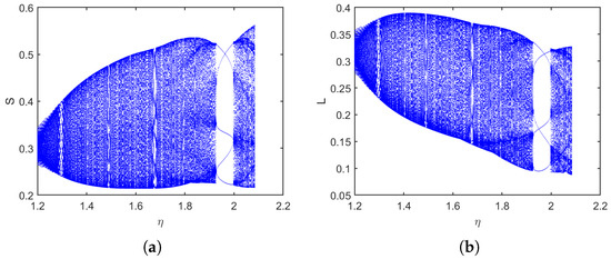
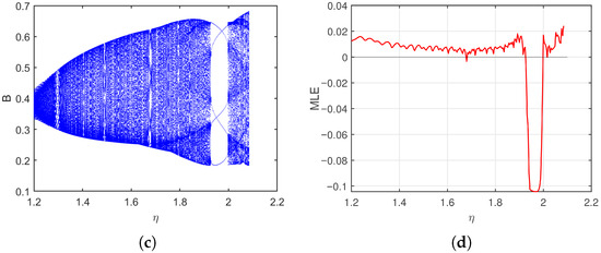
Figure 10.
Bifurcation and MLE of the discrete-time SLB model of computer viruses (2) as varies for . (a–c) Bifurcation of S, L, and B, (d) Maximum Lyapunov exponent (MLE).

Figure 11.
Phase portraits of the discrete-time SLB model (2) for , for different values: (a) , (b) , and (c) .
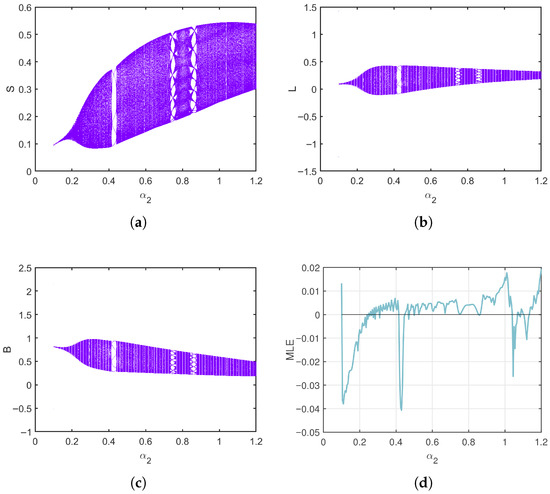
Figure 12.
Bifurcation and MLE of the discrete-time SLB model of computer viruses (2) as varies for . (a–c) Bifurcation of S, L, and B, (d) Maximum Lyapunov exponent (MLE).
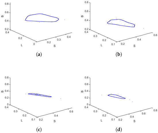
Figure 13.
Phase portraits of the discrete-time SLB model (2) for , for different values: (a) , (b) , (c) , and (d) .
When comparing the three cases, a clear relationship emerges between the parameters (the transition rate from latent to breaking-out computers) and (the cure rate of breaking-out computers) and the system’s qualitative behavior.
- Case 1 shows a gradual and predictable route to chaos. As either or increases, the system evolves from stable fixed points through period-doubling bifurcations into a chaotic regime. The Maximum Lyapunov Exponent (MLE) becomes positive in intermediate ranges, confirming the onset of chaos. This suggests that high transition or cure rates can destabilize the infection cycle when increased progressively.
- Case 2 exhibits sharp and abrupt transitions to chaos. The bifurcation diagrams reveal dense and discontinuous oscillations, and the MLE shows intermittent positivity, indicating the presence of transient chaos. Even moderate changes in or cause erratic and unpredictable system behavior. This case highlights the system’s sensitivity to small parameter variations and underscores the risks of instability associated with nonlinearity.
- Case 3 analysis of the bifurcation diagrams and MLE shows that chaos is still present across most of the parameter space. The MLE remains positive except for a small stability window, indicating short-lived regular dynamics. Phase portraits confirm the presence of chaotic attractors. Hence, even seemingly mild parameter values can lead to instability if not precisely calibrated.
From a practical perspective, these results have important implications for digital security and network design. The transition rate reflects how quickly latent threats become active. A high , especially in systems lacking early detection, can trigger unpredictable outbreaks. Likewise, although increasing the cure rate may seem beneficial, the analysis reveals that excessive or poorly tuned values can contribute to system instability, particularly when delays or nonlinear feedback are present in the recovery process. Maintaining parameters within identified stability regions, particularly in the narrow MLE-negative intervals, is essential. This study reinforces the value of bifurcation and chaos theory as diagnostic and predictive tools for analyzing computer virus models in discrete-time systems. The insights gained can inform more effective cybersecurity strategies and contribute to the design of more resilient digital infrastructures.
5. Complexity Analysis
To characterize the irregularity of the system’s time series, we employ the complexity measure [29], a frequency-domain-based indicator of chaotic behavior. The procedure begins by computing the average amplitude of the Fourier spectrum,
A threshold parameter r is then applied to filter the spectrum, yielding
where retains only the dominant spectral components.
The inverse Fourier transform reconstructs the filtered signal as
Finally, the complexity is defined by
In our simulations, the threshold parameter is selected as r = 1, which is the standard choice used in C0-complexity analysis. Low values of indicate ordered or periodic dynamics, while higher values reveal chaotic and irregular behaviors, making it a reliable tool for complexity assessment in discrete-time systems. The complexity of the discrete-time SLB model was evaluated by varying while fixing at different values with . As shown in Figure 14, increasing from to leads to more pronounced irregular fluctuations in , which indicates a higher sensitivity of the system to initial conditions. These results demonstrate that the cure rate plays a significant role in the transition to chaos, and higher values intensify the system’s complexity, in agreement with the bifurcation and phase portrait analyses.

Figure 14.
complexity of the discrete-time SLB model for: (a) , (b) , (c) .
6. Stabilization and Synchronization
To ensure stability and achieve synchronization of the proposed discrete-time SLB model, we introduce adaptive control laws designed to asymptotically drive all system states toward zero.
6.1. Stabilization
In this subsection, we’ll explore how to control the discrete-time SLB model of computer viruses described in (2) by adding a straightforward nonlinear control law. Our main goal is to stabilize the system’s dynamics by guiding all its state variables back to the virus-free fixed point. Here’s how we’ve defined the controlled version of the model:
Here, is the adaptive controller. The specific control laws for this discrete-time SLB model are then presented in the following proposition, which are derived directly from the discrete system stability conditions found in [26].
Proposition 1.
The new discrete-time SLB model is stable under the following 3D control law:
where the control parameters must satisfy the conditions: , , and . When these conditions are met, the model can be effectively stabilized at the virus-free fixed point .
Remark 1.
These conditions specify the minimum control strengths () required to stabilize the virus-free equilibrium , ensuring that the network returns to a safe state where all computers are virus-free.
Proof.
To prove Proposition 1, we substitute the control law (18) into the system given in (17). This yields the following system:
From this system, we clearly observe that the eigenvalues are , , and . According to the assumption in Proposition 1, we have , . This condition ensures that all eigenvalues lie inside the unit circle, which is the fundamental criterion for asymptotic stability in discrete-time systems. Hence, the controlled system (17) is asymptotically stable. □
Figure 15 provides a visual confirmation of this result. It depicts the evolution of the system states and visualization of the system in phase space, under the control law with parameters and initial conditions as . The figure clearly shows that the state variables of the controlled model converge asymptotically to , thereby validating the effectiveness of the proposed control strategy.
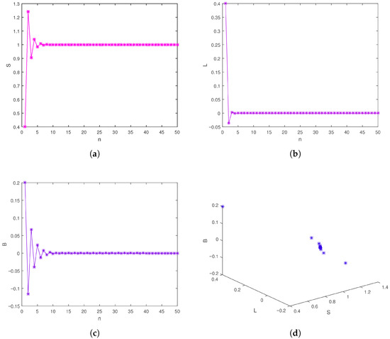
Figure 15.
(a) Stabilization of S, (b) Stabilization of L, (c) Stabilization of B, (d) Phase space.
From a practical perspective, adaptive controllers are relevant to real network infrastructures. In computer systems, infection and transmission rates are not constant; they vary due to network traffic changes, software updates, or external attacks. A nonlinear control law can automatically strengthen mitigation actions (packet filtering, node isolation, forced antivirus scans) when abnormal propagation is detected. This means that the controller acts only when needed, suppressing outbreaks and stabilizing the network while avoiding unnecessary interventions. Therefore, the proposed control scheme offers a realistic mechanism for limiting virus propagation in networks with uncertain or time-varying dynamics.
6.2. Synchronization
Synchronization of chaotic systems has attracted significant attention owing to its theoretical challenges and wide range of applications, particularly in secure communications and complex network dynamics. Within the framework of computer virus propagation, synchronization can be employed to design control mechanisms that stabilize or suppress chaotic spreading behavior.
To investigate synchronization, we consider system (2) as the master system. A corresponding slave system is constructed by introducing appropriate control inputs and as follows:
where denote the slave states.
The goal is to design the controllers such that
Proposition 2.
Proof.
Computation shows that the eigenvalues are , , and . Based on the assumption in Proposition 2, the eigenvalues satisfy , . This guarantees that all eigenvalues lie strictly within the unit circle; it can be shown that the error system is globally asymptotically stable. Thus, synchronization between the master and slave systems is ensured. □
To verify the theoretical results, numerical experiments are performed using and the system’s parameters , , , and . The synchronization errors , , are plotted in Figure 16 and shown to converge asymptotically to zero, confirming the effectiveness of the proposed control scheme.
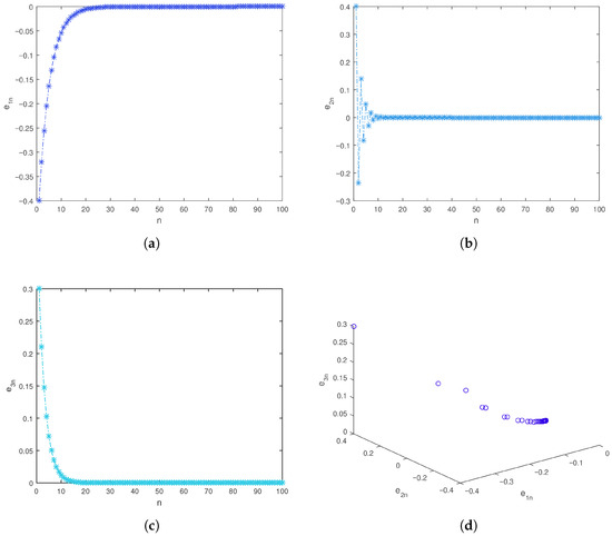
Figure 16.
(a–c)Time series of the synchronization errors, (d) Phase space.
The presence of chaotic dynamics in the discrete-time SLB model indicates that computer-virus propagation can exhibit highly unpredictable outbreaks, even under seemingly stable conditions. Understanding these dynamics allows network administrators to anticipate periods of rapid infection growth and implement targeted interventions. The proposed adaptive control and synchronization strategies demonstrate how coordinated adjustments of recovery or intervention rates can stabilize network behavior. In practice, such controllers can guide real-world cybersecurity actions, including synchronized software updates, network traffic regulation, and adaptive patch deployment, ensuring network stability and mitigating uncontrolled virus propagation. This integrated approach provides actionable guidance for network administrators and cybersecurity teams, linking theoretical insights to practical applications.
7. Conclusions and Future Works
This paper introduced and thoroughly analyzed a discrete-time SLB model for computer virus propagation, capturing the transitions between Susceptible, Latent, and Breaking-out states in internal netw orks. Stability analysis using the basic reproduction number (), combined with bifurcation diagrams, Maximum Lyapunov Exponents, and complexity, revealed rich nonlinear dynamics, including chaotic regimes and periodic windows. The proposed nonlinear control strategy successfully suppresses chaotic outbreaks, while the synchronization scheme demonstrates how coupled systems can achieve coordinated behavior.
Beyond theoretical contributions, the findings provide concrete implications for cybersecurity. The model offers a predictive framework for understanding how computer viruses propagate through networks, enabling administrators to identify critical thresholds, anticipate outbreak scenarios, and implement timely interventions. Control and synchronization strategies can be directly translated into practical measures, such as coordinated patch deployment, network traffic regulation, and adaptive defense policies, to mitigate virus spread and maintain network stability.
Future work will extend this framework to heterogeneous and large-scale network structures, incorporate adaptive and stochastic control strategies, and validate the model against real-world cyberattack data. By bridging rigorous mathematical modeling with practical cybersecurity applications, this study aims to provide both a deeper theoretical understanding and actionable guidance for managing complex virus propagation in interconnected digital environments.
Author Contributions
Conceptualization, A.A. and O.K.; Methodology, I.Z.; Software, I.Z.; Validation, O.K. and A.O.; Formal analysis, L.E.A. and M.A.; Investigation, I.Z.; Resources, L.E.A. and M.A.; Data curation, A.A. and A.O.; Writing—original draft, I.Z.; Writing—review & editing, I.Z. and O.K.; Visualization, I.Z.; Supervision, A.O.; Project administration, I.Z. and A.O.; Funding acquisition, A.A. and O.K. All authors have read and agreed to the published version of the manuscript.
Funding
Princess Nourah bint Abdulrahman University Researchers Supporting Project number (PNURSP2025R831), Princess Nourah bint Abdulrahman University, Riyadh, Saudi Arabia. The authors extend their appreciation to the Deanship of Scientific Research at Northern Border University, Arar, KSA for funding this research work through the project number “NBU- FPEJ-2025-2443-08”.
Data Availability Statement
The original contributions presented in this study are included in the article. Further inquiries can be directed to the corresponding authors.
Acknowledgments
Princess Nourah bint Abdulrahman University Researchers Supporting Project number (PNURSP2025R831), Princess Nourah bint Abdulrahman University, Riyadh, Saudi Arabia. The authors extend their appreciation to the Deanship of Scientific Research at Northern Border University, Arar, KSA for funding this research work through the project number “NBU- FPEJ-2025-2443-08”.
Conflicts of Interest
The authors declare no conflicts of interest.
References
- Murray, J.D. Mathematical Biology, 3rd ed.; Springer: Berlin/Heidelberg, Germany, 2002. [Google Scholar]
- Strogatz, S.H. Nonlinear Dynamics and Chaos: With Applications to Physics, Biology, Chemistry, and Engineering; CRC Press: Boca Raton, FL, USA, 2018. [Google Scholar]
- Chen, G.; Wang, X.; Li, X. Fundamentals of Complex Networks: Models, Structures and Dynamics; Wiley-Blackwell: Hoboken, NJ, USA, 2015. [Google Scholar]
- Haugh, J.M. Analysis of reaction–diffusion systems with anomalous subdiffusion. Biophys. J. 2009, 97, 435–442. [Google Scholar] [CrossRef]
- Na, Y.; Peng, L.; Zhang, Q. Bifurcation analysis and tracking control of an epidemic model with a nonlinear incidence rate. Appl. Math. Model. 2012, 36, 1678–1693. [Google Scholar] [CrossRef]
- Benito, B.C.C.; Dobromir, D.; Kolev, H. Numerical simulation of multi-species biofilms in porous media for different kinetics. Math. Comput. Simul. 2009, 79, 1846–1861. [Google Scholar] [CrossRef]
- Kermack, W.O.; McKendrick, A.G. Contributions to the mathematical theory of epidemics. Proc. R. Soc. Lond. A 1927, 115, 700–721. [Google Scholar]
- Hethcote, H.W. The Mathematics of Infectious Diseases. SIAM Rev. 2000, 42, 599–653. [Google Scholar] [CrossRef]
- Kephart, J.O.; White, S.R. Directed-graph epidemiological models of computer viruses. In Proceedings of the 1991 IEEE Computer Society Symposium on Research in Security and Privacy, Oakland, CA, USA, 20–22 May 1991; IEEE: Washington, DC, USA, 1991; pp. 343–359. [Google Scholar]
- Anderson, R.M.; May, R.M. Infectious Diseases of Humans: Dynamics and Control; Oxford University Press: Oxford, UK, 1991. [Google Scholar]
- Tang, W.; Yang, H.; Pi, J. Dynamics and control strategies for SLBRS model of computer viruses based on complex networks. Int. J. Intell. Syst. 2024, 2024, 3943882. [Google Scholar] [CrossRef]
- Quiroga-Sánchez, L.; Montoya, G.A.; Lozano-Garzón, C. The SEIRS-NIMFA epidemiological model for malware propagation analysis in IoT networks. Cybersecurity 2025, 8, 2. [Google Scholar] [CrossRef]
- Fang, Z.; Zhao, P.; Xu, M.; Xu, S.; Hu, T.; Fang, X. Statistical modelling of computer malware propagation dynamics in cyberspace. J. Appl. Stat. 2020, 49, 858–883. [Google Scholar] [CrossRef]
- Xu, X.-J.; Peng, H.-O.; Wang, X.-M.; Wang, Y.-H. Epidemic spreading with time delay in complex networks. Phys. A Stat. Mech. Its Appl. 2006, 367, 525–530. [Google Scholar] [CrossRef]
- Mishra, B.K.; Saini, D.K. SEIRS epidemic model with delay for transmission of malicious objects in a computer network. Appl. Math. Comput. 2007, 188, 1476–1482. [Google Scholar] [CrossRef]
- Zhang, Z.; Kumari, S.; Upadhyay, R.K. A delayed e-epidemic SLBS model for computer virus. Adv. Differ. Equ. 2019, 2019, 414. [Google Scholar] [CrossRef]
- Zhang, Z.; Yang, H. Stability and Hopf bifurcation for a delayed SLBRS computer virus model. Sci. World J. 2014, 2014, 373171. [Google Scholar] [CrossRef] [PubMed]
- Abu Hammad, M.; Zouak, I.; Ouannas, A.; Grassi, G. Fractional discrete computer virus system: Chaos and complexity algorithms. Algorithms 2025, 18, 444. [Google Scholar] [CrossRef]
- Kahouli, O.; Zouak, I.; Ouannas, A.; Abidi, I.; Bahou, Y.; Elgharbi, S.; Chaabane, M. Control and synchronization of chaos in some fractional computer virus models. Asian J. Control 2025, 1–9. [Google Scholar] [CrossRef]
- Kahouli, O.; Zouak, I.; Hammad, M.A.; Ouannas, A. Chaos, control, and synchronization in a discrete-time computer virus system with fractional orders. AIMS Math. 2025, 10, 13594–13621. [Google Scholar] [CrossRef]
- Yang, L.-X.; Yang, X.; Liu, J.; Zhu, Q.; Gan, C. Epidemics of computer viruses: A complex-network approach. Appl. Math. Comput. 2013, 219, 8705–8717. [Google Scholar] [CrossRef]
- Zhou, Y.; Wang, Y.; Zhou, K.; Shen, S.-F.; Ma, W.-X. Dynamical behaviors of an epidemic model for malware propagation in wireless sensor networks. Front. Phys. 2023, 11, 1198410. [Google Scholar] [CrossRef]
- Kahouli, O.; Zouak, I.; Abu Hammad, M.; Ouannas, A.; Ayari, M. On an incommensurate chaotic fractional discrete model of a computer virus: Stabilization and synchronization. AIMS Math. 2025, 10, 19940–19957. [Google Scholar] [CrossRef]
- Zouak, I.; Alshanty, A.; Ouannas, A.; Mongelli, A.; Ciccarese, G.; Grassi, G. From Continuous Integer-Order to Fractional Discrete-Time: A New Computer Virus Model with Chaotic Dynamics. Technologies 2025, 13, 471. [Google Scholar] [CrossRef]
- Yang, L.X.; Yang, X.; Zhu, Q.; Wen, L. A computer virus model with grader cure rates. Nonlinear Anal. Real World Appl. 2013, 14, 414–422. [Google Scholar] [CrossRef]
- Elaydi, S. An Introduction to Difference Equations, 3rd ed.; Springer SBM: Berlin/Heidelberg, Germany, 2005. [Google Scholar]
- Masood, Z.; Raja, M.A.Z.; Chaudhary, N.I.; Cheema, K.M.; Milyani, A.H. Fractional dynamics of Stuxnet virus propagation in industrial control systems. Mathematics 2021, 9, 2160. [Google Scholar] [CrossRef]
- Wu, G.-C.; Baleanu, D. Jacobian matrix algorithm for Lyapunov exponents of the discrete fractional maps. Commun. Nonlinear Sci. 2015, 22, 95–100. [Google Scholar] [CrossRef]
- Shen, E.; Cai, Z.; Gu, F. Mathematical foundation of a new complexity measure. Appl. Math. Mech. 2005, 26, 1188–1196. [Google Scholar] [CrossRef]
Disclaimer/Publisher’s Note: The statements, opinions and data contained in all publications are solely those of the individual author(s) and contributor(s) and not of MDPI and/or the editor(s). MDPI and/or the editor(s) disclaim responsibility for any injury to people or property resulting from any ideas, methods, instructions or products referred to in the content. |
© 2025 by the authors. Licensee MDPI, Basel, Switzerland. This article is an open access article distributed under the terms and conditions of the Creative Commons Attribution (CC BY) license (https://creativecommons.org/licenses/by/4.0/).