Several Subordination Features Using Bessel-Type Operator

Abstract

For the function solution to the well-known homogeneous Bessel differential equation, we utilized a normalized form of this function to define a certain operator on a subclass of analytic functions. Using this operator, we introduced various subordination properties. We also examined the sufficient starlikeness conditions and provided some estimates for a specific subclass of univalent functions defined in the unit disc.

1. Introduction

Consider $\mathcal{F}$ to represent the family of analytic and univalent functions in the open unit disc $▿:=\{\zeta \in \mathbb{C}:|\zeta |<1\}$, with the following series representation:

$$f(\zeta )=\zeta +{\displaystyle \sum _{n=1}^{\infty }}{a}_{n+1}{\zeta }^{n+1}.$$

(1)

The solution for the differential equation ([1])

$${\zeta }^2{w}^{″}(\zeta )+b\zeta w^{\prime }(\zeta )+\left[c{\zeta }^2-p^2+(1-b)p\right]w(\zeta )=0\left(b,c,p\in \mathbb{C}\right),$$

(2)

is $w_{b,c,p}\left(\zeta \right)$, which is the generalized Bessel function, and has the following representation:

$$w_{b,c,p}(\zeta )={\displaystyle \sum _{n=0}^{\infty }}{\displaystyle \frac{{(-c)}^n}{n!\mathsf{\Gamma }\left(n+p+\frac{b+1}{2}\right)}}{\left({\displaystyle \frac{\zeta }{2}}\right)}^{2n+p},$$

(3)

for $b,c,p,\zeta \in \mathbb{C}$, and $p+{\displaystyle \frac{b+1}{2}}\in \mathbb{C}\setminus {\mathbb{Z}}_0^{-},$${\mathbb{Z}}_0^{-}=\left\{0,-1,-2,\dots \right\}$. Classical, modified, and spherical Bessel functions can all be studied in a unified way through series (3), as follows:

(i)

Acquiring $c=b=1$ within (3) gives the familiar Bessel function of the first kind of order p defined by Watson [2] (Baricz [1]):

$$J_p(\zeta )={\displaystyle \sum _{n=0}^{\infty }}{\displaystyle \frac{{(-1)}^n}{n!\mathsf{\Gamma }\left(p+n+1\right)}}{\left({\displaystyle \frac{\zeta }{2}}\right)}^{2n+p};\zeta \in \mathbb{C}.$$

(ii)

Acquiring $c=-1$ and $b=1$ within (3) gives the modified Bessel function of the first kind of order p given as ([1,2])

$$I_p(\zeta )={\displaystyle \sum _{n=0}^{\infty }}{\displaystyle \frac{1}{n!\mathsf{\Gamma }\left(p+n+1\right)}}{\left({\displaystyle \frac{\zeta }{2}}\right)}^{2n+p};\zeta \in \mathbb{C}.$$

(iii)

Acquiring $c=1$ and $b=2$ within (3) gives the spherical Bessel function of the first kind of order p expressed as ([1])

$$j_p(\zeta )=\sqrt{{\displaystyle \frac{\pi }{2}}}{\displaystyle \sum _{n=0}^{\infty }}{\displaystyle \frac{{(-1)}^n}{n!\mathsf{\Gamma }\left(p+n+\frac{3}{2}\right)}}{\left({\displaystyle \frac{\zeta }{2}}\right)}^{2n+p};\zeta \in \mathbb{C}.$$

Now, we employ the function ${\phi }_{b,c,p}\left(\zeta \right)$, which is a normalization for $w_{b,c,p}\left(\zeta \right)$, with the following ([3,4]):

$${\phi }_{b,c,p}(\zeta )=2^p\mathsf{\Gamma }\left(p+{\displaystyle \frac{b+1}{2}}\right){\zeta }^{1-{\displaystyle \frac{p}{2}}}{w}_{b,c,p}(\sqrt{\zeta })\left(b,c,p\in \mathbb{C},p+\frac{b+1}{2}\in \mathbb{C}\setminus {\mathbb{Z}}_0^{-}\right).$$

(4)

Thus, ${\phi }_{b,c,p}(\zeta )$ takes the following series form:

$${\phi }_{\kappa ,c}(\zeta )=\zeta +{\displaystyle \sum _{n=1}^{\infty }}{\displaystyle \frac{{(-c)}^n}{4^n{\left(\kappa \right)}_n}}{\displaystyle \frac{{\zeta }^{n+1}}{n!}}\left(\kappa =p+{\displaystyle \frac{b+1}{2}}\in \mathbb{C}\setminus {\mathbb{Z}}_0^{-},b,c,p\in \mathbb{C}\right).$$

(5)

Now, the convolution-type operator

$${\mathcal{B}}_{\kappa }^c:\mathcal{F}⟶\mathcal{F},$$

is defined as follows:

$$\begin{array}{cc}\hfill & \begin{array}{c}{\mathcal{B}}_{\kappa }^{c}f(\zeta ):={\phi }_{\kappa ,c}(\zeta )\ast f(\zeta )\end{array}\hfill \\ \hfill & \begin{array}{c}=\zeta +{\displaystyle \sum _{n=1}^{\infty }}{\displaystyle \frac{{(-c)}^n{a}_{n+1}}{4^n{\left(\kappa \right)}_n}}{\displaystyle \frac{{\zeta }^{n+1}}{n!}},\end{array}\hfill \end{array}$$

(6)

where ${\left(\kappa \right)}_n$ refers to the Pochhammer (shifted factorial), which is expressed as

$${\left(\kappa \right)}_n={\displaystyle \frac{\mathsf{\Gamma }\left(\kappa +n\right)}{\mathsf{\Gamma }\left(\kappa \right)}}=\left\{\begin{array}{l}1,\left(n=0,\kappa \in \mathbb{C}\setminus \left\{0\right\}\right),\\ \kappa \left(\kappa +1\right)\dots \left(\kappa +n-1\right),\left(n\in \mathbb{N},\kappa \in \mathbb{C}\right).\end{array}\right.$$

Applying (6),

$$\zeta {\left({\mathcal{B}}_{\kappa }^{c}f(\zeta )\right)}^{\prime }=\left(\kappa -1\right){\mathcal{B}}_{\kappa -1}^{c}f(\zeta )-\left(\kappa -2\right){\mathcal{B}}_{\kappa }^{c}f(\zeta ).$$

(7)

We list some operators as special cases:

(i)

By acquiring $c=-4$ in (6), we obtain the operator ${\mathcal{N}}_{\kappa }:\mathcal{F}⟶\mathcal{F}$, defined by

$${\mathcal{N}}_{\kappa }f(\zeta )=\zeta +\sum _{n=1}^{\infty }{\displaystyle \frac{a_{n+1}}{{\left(\kappa \right)}_n}}{\displaystyle \frac{{\zeta }^{n+1}}{n!}};\kappa \in \mathbb{C}\setminus {\mathbb{Z}}_0^{-};$$

(8)

(ii)

By acquiring $c=b=1$ in (6), we arrive to the operator ${\mathcal{J}}_p:\mathcal{F}⟶\mathcal{F}$, defined by

$${\mathcal{J}}_{p}f(\zeta )=\zeta +\sum _{n=1}^{\infty }{\displaystyle \frac{{(-1)}^n{a}_{n+1}}{4^n{\left(p+1\right)}_n}}{\displaystyle \frac{{\zeta }^{n+1}}{n!}};p+1\in \mathbb{C}\setminus {\mathbb{Z}}_0^{-};$$

(9)

(iii)

By acquiring $c=-1$ and $b=1$ in (6), we have the operator ${\mathcal{I}}_p:\mathcal{F}⟶\mathcal{F}$, defined by

$${\mathcal{I}}_{p}f(\zeta )=\zeta +\sum _{n=1}^{\infty }{\displaystyle \frac{a_{n+1}}{4^n{\left(p+1\right)}_n}}{\displaystyle \frac{{\zeta }^{n+1}}{n!}};p+1\in \mathbb{C}\setminus {\mathbb{Z}}_0^{-};$$

(10)

(iv)

By acquiring $c=1$ and $b=2$ in (6), we have the operator ${\mathcal{S}}_p:\mathcal{F}⟶\mathcal{F},$ defined by

$${\mathcal{S}}_{p}f(\zeta )=\zeta +\sum _{n=1}^{\infty }{\displaystyle \frac{{(-1)}^n{a}_{n+1}}{4^n{\left(p+\frac{3}{2}\right)}_n}}{\displaystyle \frac{{\zeta }^{n+1}}{n!}};p+{\displaystyle \frac{3}{2}}\in \mathbb{C}\setminus {\mathbb{Z}}_0^{-}.$$

(11)

Now, and with the help of the operator ${\mathcal{B}}_{\kappa }^c$, in the following definition, we define a subclass of functions $S_{\kappa }^c\left(\alpha ;C,D\right)\subset \mathcal{F}$. The investigations within this paper are focused on studying the properties of functions belonging to this subclass.

Definition 1. 

For real $-1\le D<C\le 1$, $0\le \alpha <1$ and $f\in \mathcal{F}$, $f\in S_{\kappa }^c\left(\alpha ;C,D\right)$ if it fulfills the subordination:

$${\displaystyle \frac{1}{1-\alpha }}\left({\displaystyle \frac{\zeta {\left({\mathcal{B}}_{\kappa }^{c}f(\zeta )\right)}^{\prime }}{{\mathcal{B}}_{\kappa }^{c}f(\zeta )}}-\alpha \right)\prec {\displaystyle \frac{1+C\zeta }{1+D\zeta }}.$$

(12)

Alternatively, in a similar way,

$$\begin{array}{cc}\hfill & \begin{array}{c}{S}_{\kappa }^c\left(\alpha ;C,D\right)=\left\{f\in \mathcal{F}:\left|\frac{{\displaystyle \frac{\zeta {\left({\mathcal{B}}_{\kappa }^{c}f(\zeta )\right)}^{\prime }}{{\mathcal{B}}_{\kappa }^{c}f(\zeta )}}-1}{D{\displaystyle \frac{\zeta {\left({\mathcal{B}}_{\kappa }^{c}f(\zeta )\right)}^{\prime }}{{\mathcal{B}}_{\kappa }^{c}f(\zeta )}}-\left[D+(C-D)(1-\alpha )\right]}\right|<1;\zeta \in ▿\right\}.\end{array}\hfill \\ \hfill & \begin{array}{c}\left(-1\le D<C\le 1;0\le \alpha <1;\kappa =p+{\displaystyle \frac{b+1}{2}}\in \mathbb{C}\setminus {\mathbb{Z}}_0^{-};b,c,p\in \mathbb{C}\right)\end{array}\hfill \end{array}$$

Additionally, for $C=-D=1$, we write $S_{\kappa }^c\left(\alpha ;1,-1\right)=S_{\kappa }^c\left(\alpha \right)$, where

$$S_{\kappa }^c\left(\alpha \right)=\left\{f\in \mathcal{F}:\Re \left\{{\displaystyle \frac{\zeta {\left({\mathcal{B}}_{\kappa }^{c}f(\zeta )\right)}^{\prime }}{{\mathcal{B}}_{\kappa }^{c}f(\zeta )}}\right\}>\alpha ;\zeta \in ▿\right\}.$$

(13)

We recommend the papers [1,4,5,6,7,8] for additional results on the modification of the generalized Bessel function. These papers established a variety of functional inequalities, integral representations, extensions of some known trigonometric inequalities, starlikeness, convexity, and univalence. Using the normalized form of the first-kind ordinary Bessel function and the normalized form of the first-kind generalized Bessel functions, respectively, Baricz and Frasin [7] and Deniz et al. [4] were interested in the univalence of certain integral operators. Several sufficient circumstances for the convexity and strong convexity of the integral operators formed by the normalized expression of the ordinary Bessel function of the first kind were obtained by Frasin [9]. Additionally, numerous authors have addressed the issue of some generalized integral operators’ geometric features (such as convexity, starlikeness, and univalence). In addition, we recommend [10,11,12,13,14,15,16,17,18]. For more recent works about Bessel functions, we refer to [19,20,21,22,23].

The primary objective of this work is to introduce a variety of subordination properties involving the linear operator ${\mathcal{B}}_{\kappa }^c$ associated with the generalized Bessel functions defined by (6). Also, we investigated some estimates and sufficient starlike conditions of certain subclass of univalent functions defined in ▿.

2. Preliminaries

We start by going over each of the next lemmas, which are necessary for our current study.

Lemma 1 

([24,25]). Let h be a convex (univalent) analytic function in ▿ such that $h(0)=1$. Assume, further, that the function ϕ is analytic and denoted by

$$\varphi (\zeta )=1+c_1\zeta +c_2{\zeta }^2+\dots .$$

(14)

If

$$\varphi (\zeta )+{\displaystyle \frac{\zeta {\varphi }^{\prime }(\zeta )}{\delta }}\prec h(\zeta )\left(\delta \ne 0,\Re \left\{\delta \right\}\ge 0,\zeta \in ▿\right),$$

then

$$\varphi (\zeta )\prec \psi (\zeta )={\displaystyle \frac{\delta }{{\zeta }^{\delta }}}\underset{0}{\overset{\zeta }{\int }}{t}^{\delta -1}h(t)dt\prec h(\zeta )\left(\delta \ne 0,\Re \left\{\delta \right\}\ge 0,\zeta \in ▿\right),$$

(15)

and $\psi (\zeta )$ is the best dominant of (15).

Lemma 2 

([25]). For $\mathsf{\Psi }:{\mathbb{C}}^2\times ▿⟶\mathbb{C}$ fulfills the subsequent requirement:

$$\Re \left\{\mathsf{\Psi }\left(ix,y;\zeta \right)\right\}\le \epsilon ,$$

for all $x\in \mathbb{R}$ and $y\le -{\displaystyle \frac{1}{2}}\left(1+x^2\right),$ and for all $\zeta \in ▿.$ If the function ϕ of the form (14) is analytic in ▿ and

$$\Re \left\{\mathsf{\Psi }\left(\varphi (\zeta ),\zeta {\varphi }^{\prime }(\zeta );\zeta \right)\right\}>\epsilon \left(\zeta \in ▿\right),$$

this leads to

$$\Re \left\{\varphi (\zeta )\right\}>0\left(\zeta \in ▿\right).$$

Lemma 3 

([26]). Let $\lambda \in \mathbb{R}\setminus \left\{0\right\}$, $0\le \beta <1$ and $a\lambda >0$. Additionally, assume that $\mathsf{\Psi }(\zeta )=1+c_n{\zeta }^n+c_{n+1}{\zeta }^{n+1}+\dots$ is analytic in ▿, and

$$\mathsf{\Psi }(\zeta )\prec 1+{\displaystyle \frac{aM}{n\lambda +a}}\zeta \left(n\in \mathbb{N}\right),$$

where

$$M={\displaystyle \frac{\left(1-\beta \right)\left|\lambda \right|\left(1+\frac{n\lambda }{a}\right)}{\left|1-\lambda +\lambda \beta \right|+\sqrt{1+{\left(1+\frac{n\lambda }{a}\right)}^2}}}.$$

If the function $\theta (\zeta )=1+d_n{\zeta }^n+d_{n+1}{\zeta }^{n+1}+\dots$ is analytic in ▿ and satisfies

$$\mathsf{\Psi }(\zeta )\left\{1-\lambda +\lambda \left[\left(1-\beta \right)\theta (\zeta )+\beta \right]\right\}\prec 1+M\zeta ,$$

this gives that

$$\Re \left\{\theta (\zeta )\right\}>0\left(\zeta \in ▿\right).$$

Let $P\left(\gamma \right)$ be the family of all functions $\varphi$ expressed with (14), analytic in ▿, and that satisfies $\Re \left\{\varphi (\zeta )\right\}>\gamma$$\left(0\le \gamma <1,\zeta \in ▿\right).$

Lemma 4 

([27]). If $\varphi \in P\left(\gamma \right)$, then

$$\Re \left\{\varphi (\zeta )\right\}>2\gamma -1+{\displaystyle \frac{2\left(1-\gamma \right)}{1+\left|\zeta \right|}}\left(0\le \gamma <1,\zeta \in ▿\right).$$

Lemma 5 

([28]). Let the functions $\varphi \in P\left({\gamma }_1\right)$ and $\psi \in P\left({\gamma }_2\right)$ be such that $0\le {\gamma }_1<{\gamma }_2<1$. Then,

$$\varphi \ast \psi \in P\left({\gamma }_3\right),$$

where ${\gamma }_3=1-2\left(1-{\gamma }_1\right)\left(1-{\gamma }_2\right)$.

For complex numbers ${\alpha }_1$, ${\alpha }_2$, and ${\beta }_1\left({\beta }_1\notin {\mathbb{Z}}_0^{-}\right)$, the Gauss hypergeometric function is given in [29] (Chapter 14):

$${}_{2}F_1\left({\alpha }_1,{\alpha }_2;{\beta }_1;\zeta \right)=1+{\displaystyle \frac{{\alpha }_1{\alpha }_2}{{\beta }_1}}{\displaystyle \frac{\zeta }{1!}}+{\displaystyle \frac{{\alpha }_1\left({\alpha }_1+1\right){\alpha }_2\left({\alpha }_2+1\right)}{{\beta }_1\left({\beta }_1+1\right)}}{\displaystyle \frac{{\zeta }^2}{2!}}+\dots$$

Lemma 6 

([29]). For any complex parameters ${\alpha }_1$, ${\alpha }_2$, and ${\beta }_1\left({\beta }_1\notin {\mathbb{Z}}_0^{-}\right)$, the following equalities hold:

$${\int }_0^1{t}^{{\alpha }_2-1}{\left(1-t\right)}^{{\beta }_1-{\alpha }_2-1}{\left(1-\zeta t\right)}^{-{\alpha }_1}dt={\displaystyle \frac{\mathsf{\Gamma }({\alpha }_2)\mathsf{\Gamma }({\beta }_1-{\alpha }_2)}{\mathsf{\Gamma }({\beta }_1)}}\begin{array}{c}{}_{2}F_1\left({\alpha }_1,{\alpha }_2;{\beta }_1;\zeta \right),\end{array}$$

(16)

where $\Re \left\{{\beta }_1\right\}>\Re \left\{{\alpha }_2\right\}>0$ and $\zeta \in ▿$. Also,

$${}_{2}F_1\left({\alpha }_1,{\alpha }_2;{\beta }_1;\zeta \right)=\begin{array}{c}{}_{2}F_1\left({\alpha }_2,{\alpha }_1;{\beta }_1;\zeta \right),\end{array}$$

(17)

and

$${}_{2}F_1\left({\alpha }_1,{\alpha }_2;{\beta }_1;\zeta \right)={\left(1-\zeta \right)}^{-{\alpha }_1}\begin{array}{c}{}_{2}F_1\left({\alpha }_1,{\beta }_1-{\alpha }_2;{\beta }_1;{\displaystyle \frac{\zeta }{\zeta -1}}\right).\end{array}$$

(18)

3. Subordination Properties Involving ${\mathcal{B}}_{\mathit{\kappa }}^{\mathit{c}}$

Throughout this article, unless specified otherwise, $-1\le D<C\le 1$; $0\le \alpha <1$; $\kappa =p+{\displaystyle \frac{b+1}{2}}\in \mathbb{R}\setminus {\mathbb{Z}}_0^{-}$; $b,c,p\in \mathbb{R}$; and $\zeta \in ▿$. We use the operator ${\mathcal{B}}_{\kappa }^c$ to introduce certain convolution and subordination features.

Theorem 1. 

Assume $\lambda >0$ and $-1\le D_j<C_j\le 1$. If $f_j\in \mathcal{F}$ fulfill the subordination,

$$\left(1-\lambda \right){\displaystyle \frac{{\mathcal{B}}_{\kappa }^c{f}_j(\zeta )}{\zeta }}+\lambda {\displaystyle \frac{{\mathcal{B}}_{\kappa -1}^c{f}_j(\zeta )}{\zeta }}\prec {\displaystyle \frac{1+C_j\zeta }{1+D_j\zeta }}\left(forj=1,2\right),$$

(19)

Then,

$$\left(1-\lambda \right){\displaystyle \frac{{\mathcal{B}}_{\kappa }^{c}F(\zeta )}{\zeta }}+\lambda {\displaystyle \frac{{\mathcal{B}}_{\kappa -1}^{c}F(\zeta )}{\zeta }}\prec {\displaystyle \frac{1+\left(1-2{\eta }_0\right)\zeta }{1-\zeta }},$$

where $F(\zeta )={\mathcal{B}}_{\kappa }^c\left(f_1\ast f_2\right)(\zeta )$. Also,

$${\eta }_0=1-{\displaystyle \frac{4(C_1-D_1)(C_2-D_2)}{(1-D_1)(1-D_2)}}\left[1-{\displaystyle \frac{1}{2}}{}_{2}F_1\left(1,1;{\displaystyle \frac{\kappa -1}{\lambda }}+1;{\displaystyle \frac{1}{2}}\right)\right].$$

(20)

Also, in the case of $D_j=-1$, we obtain the best possible subordinating consequence.

Proof. 

Let $f_j\in \mathcal{F}$ satisfy (19). Also,

$${\phi }_j(\zeta )=\left(1-\lambda \right){\displaystyle \frac{{\mathcal{B}}_{\kappa }^c{f}_j(\zeta )}{\zeta }}+\lambda {\displaystyle \frac{{\mathcal{B}}_{\kappa -1}^c{f}_j(\zeta )}{\zeta }}\left(j=1,2\right),$$

(21)

gives

$${\phi }_j\in P({\gamma }_j)({\gamma }_j=\frac{1-C_j}{1-D_j}).$$

Using (7) and (21),

$${\mathcal{B}}_{\kappa }^c{f}_j(\zeta )=\frac{\kappa -1}{\lambda }{\zeta }^{1-\frac{\kappa -1}{\lambda }}\underset{0}{\overset{\zeta }{\int }}{t}^{{\displaystyle \frac{\kappa -1}{\lambda }}-1}{\phi }_j(t)dt,$$

(22)

if $F(\zeta )={\mathcal{B}}_{\kappa }^c\left(f_1\ast f_2\right)(\zeta )$, applying (22) and making use of

$${\mathcal{B}}_{\kappa }^{c}F(\zeta )={\mathcal{B}}_{\kappa }^c\left({\mathcal{B}}_{\kappa }^c\left(f_1\ast f_2\right)(\zeta )\right)={\mathcal{B}}_{\kappa }^c\left(f_1\right)\left(\zeta \right)\ast {\mathcal{B}}_{\kappa }^c\left(f_2\right)(\zeta ),$$

Simple computations show that

$${\mathcal{B}}_{\kappa }^{c}F(\zeta )={\displaystyle \frac{\kappa -1}{\lambda }}{\zeta }^{1-{\displaystyle \frac{\kappa -1}{\lambda }}}\underset{0}{\overset{\zeta }{\int }}{t}^{{\displaystyle \frac{\kappa -1}{\lambda }}-1}{\phi }_0(t)dt,$$

where

$${\phi }_0(\zeta )=\left(1-\lambda \right)\frac{{\mathcal{B}}_{\kappa }^{c}F(\zeta )}{\zeta }+\lambda \frac{{\mathcal{B}}_{\kappa -1}^{c}F(\zeta )}{\zeta }=\frac{\kappa -1}{\lambda }{\zeta }^{-{\displaystyle \frac{\kappa -1}{\lambda }}}\underset{0}{\overset{\zeta }{\int }}{t}^{{\displaystyle \frac{\kappa -1}{\lambda }}-1}({\phi }_1\ast {\phi }_2)(t)dt.$$

(23)

Given that ${\phi }_1\in P({\gamma }_1)$ and ${\phi }_2\in P({\gamma }_2)$, Lemma 5 implies that

$${\phi }_1\ast {\phi }_2\in P({\gamma }_3)\mathrm{with}{\gamma }_3=1-2(1-{\gamma }_1)(1-{\gamma }_2),$$

and the bound ${\gamma }_3$ is the best. Applying Lemma 4 to (23),

$$\begin{array}{cc}\hfill \Re \left\{{\phi }_0(\zeta )\right\}& ={\displaystyle \frac{\kappa -1}{\lambda }}\underset{0}{\overset{1}{\int }}{u}^{{\displaystyle \frac{\kappa -1}{\lambda }}-1}\Re \left\{(p_1\ast p_2)(u\zeta )\right\}du\hfill \\ \hfill & \ge {\displaystyle \frac{\kappa -1}{\lambda }}\underset{0}{\overset{1}{\int }}{u}^{{\displaystyle \frac{\kappa -1}{\lambda }}-1}\left[2{\gamma }_3-1+{\displaystyle \frac{2(1-{\gamma }_3)}{1+u\left|\zeta \right|}}\right]du\hfill \\ \hfill & >{\displaystyle \frac{\kappa -1}{\lambda }}\underset{0}{\overset{1}{\int }}{u}^{{\displaystyle \frac{\kappa -1}{\lambda }}-1}\left[2{\gamma }_3-1+{\displaystyle \frac{2(1-{\gamma }_3)}{1+u}}\right]du\hfill \\ \hfill & =1-{\displaystyle \frac{4(C_1-D_1)(C_2-D_2)}{(1-D_1)(1-D_2)}}\left(1-{\displaystyle \frac{\kappa -1}{\lambda }}\underset{0}{\overset{1}{\int }}{\displaystyle \frac{u^{\frac{\kappa -1}{\lambda }-1}}{1+u}}du\right)\hfill \\ \hfill & ={\eta }_0,\hfill \end{array}$$

where ${\eta }_0$ is expressed in (20). If $D_1=D_2=-1$, $f_j\in \mathcal{F}$ fulfills (19) and

$${\mathcal{B}}_{\kappa }^c{f}_j(\zeta )={\displaystyle \frac{\kappa -1}{\lambda }}{\zeta }^{1-{\displaystyle \frac{\kappa -1}{\lambda }}}\underset{0}{\overset{\zeta }{\int }}{t}^{{\displaystyle \frac{\kappa -1}{\lambda }}-1}{\displaystyle \frac{1+C_{j}t}{1-t}}dt,$$

Then, Lemmas 4 and 6 lead to

$$\begin{array}{cc}\hfill {\phi }_0(\zeta )& ={\displaystyle \frac{\kappa -1}{\lambda }}\underset{0}{\overset{1}{\int }}{u}^{{\displaystyle \frac{\kappa -1}{\lambda }}-1}\left(1-(1+C_1)(1+C_2)+{\displaystyle \frac{(1+C_1)(1+C_2)}{1-u\zeta }}\right)du\hfill \\ \hfill & =1-(1+C_1)(1+C_2)+(1+C_1)(1+C_2){(1-\zeta )}^{-1}\begin{array}{c}{}_{2}F_1\left(1,1;{\displaystyle \frac{\kappa -1}{\lambda }}+1;{\displaystyle \frac{\zeta }{\zeta -1}}\right)\end{array}\hfill \\ \hfill & \to 1-(1+C_1)(1+C_2)+{\displaystyle \frac{1}{2}}(1+C_1)(1+C_2)\begin{array}{c}{}_{2}F_1\left(1,1;{\displaystyle \frac{\kappa -1}{\lambda }}+1;{\displaystyle \frac{1}{2}}\right)\end{array}\mathrm{as}\zeta \to 1^{-},\hfill \end{array}$$

which concludes Theorem 1 exactly. □

Let $C_j=1-2{\eta }_j$, $D_j=-1(0\le {\eta }_j<1;j\in \{1,2\})$, and $\lambda =1$ in Theorem 1. Then, we have the subsequent corollary.

Corollary 1. 

Let $f_j\in \mathcal{F}$, $(j=1,2)$, fulfill

$$\Re \left\{{\displaystyle \frac{{\mathcal{B}}_{\kappa -1}^c{f}_j(\zeta )}{\zeta }}\right\}>{\eta }_j\left(0\le {\eta }_j<1,j=1,2\right),$$

Then,

$$\Re \left\{{\displaystyle \frac{{\mathcal{B}}_{\kappa -1}^{c}F(\zeta )}{\zeta }}\right\}>{\eta }_0^{\ast },$$

where $F(\zeta )={\mathcal{B}}_{\kappa }^c\left(f_1\ast f_2\right)(\zeta )$ and ${\eta }_0^{\ast }=1-4(1-{\eta }_1)(1-{\eta }_2)\left[1-\frac{1}{2}{}_{2}F_1\left(1,1;\kappa ;{\displaystyle \frac{1}{2}}\right)\right].$

Theorem 2. 

Let $\lambda >0$ and the function $f\in \mathcal{F}$ satisfy the following subordination condition:

$$(1-\lambda ){\displaystyle \frac{{\mathcal{B}}_{\kappa }^{c}f(\zeta )}{\zeta }}+\lambda {\displaystyle \frac{{\mathcal{B}}_{\kappa -1}^{c}f(\zeta )}{\zeta }}\prec {\displaystyle \frac{1+C\zeta }{1+D\zeta }}.$$

(24)

Then,

$$\Re \left\{{\left({\displaystyle \frac{{\mathcal{B}}_{\kappa }^{c}f(\zeta )}{\zeta }}\right)}^{{\displaystyle \frac{1}{\sigma }}}\right\}>{\tau }^{{\displaystyle \frac{1}{\sigma }}}(\sigma \in \mathbb{N}),$$

(25)

where

$$\tau =\left\{\begin{array}{cc}{\displaystyle \frac{C}{D}}+(1-{\displaystyle \frac{C}{D}}){(1-D)}^{-1}\begin{array}{c}{}_{2}F_1\left(1,1;{\displaystyle \frac{\kappa -1}{\lambda }}+1;{\displaystyle \frac{D}{D-1}}\right),\end{array}\hfill & (D\ne 0),\hfill \\ 1-{\displaystyle \frac{\kappa -1}{\kappa -1+\lambda }}C,\hfill & (D=0).\hfill \end{array}\right.$$

The subordination is the best possible solution.

Proof. 

Let

$$\varphi (\zeta )={\displaystyle \frac{{\mathcal{B}}_{\kappa }^{c}f(\zeta )}{\zeta }}(f\in \mathcal{F}),$$

(26)

Consequently, $\varphi$ is analytic in ▿ and takes the representation in (14). Differentiating (26) and applying (7), we arrive to

$${\displaystyle \frac{{\mathcal{B}}_{\kappa -1}^{c}f(\zeta )}{\zeta }}=\varphi (\zeta )+{\displaystyle \frac{\zeta {\varphi }^{\prime }(\zeta )}{\kappa -1}}.$$

(27)

From (24), (26), and (27), we get

$$\varphi (\zeta )+{\displaystyle \frac{\lambda }{\kappa -1}}\zeta {\varphi }^{\prime }(\zeta )\prec {\displaystyle \frac{1+C\zeta }{1+D\zeta }}.$$

Using Lemma 1,

$${\displaystyle \frac{{\mathcal{B}}_{\kappa }^{c}f(\zeta )}{\zeta }}\prec Q(\zeta )={\displaystyle \frac{\kappa -1}{\lambda }}{\zeta }^{-\frac{\kappa -1}{\lambda }}{\displaystyle \underset{0}{\overset{\zeta }{\int }}}{t}^{\frac{\kappa -1}{\lambda }-1}\left({\displaystyle \frac{1+Ct}{1+Dt}}\right)dt$$

$$=\left\{\begin{array}{cc}{\displaystyle \frac{C}{D}}+(1-{\displaystyle \frac{C}{D}}){(1-D\zeta )}^{-1}\begin{array}{c}{}_{2}F_1\left(1,1;{\displaystyle \frac{\kappa -1}{\lambda }}+1;{\displaystyle \frac{D\zeta }{1+D\zeta }}\right),\end{array}\hfill & (D\ne 0),\hfill \\ 1+{\displaystyle \frac{\kappa -1}{\kappa -1+\lambda }}C\zeta ,\hfill & (D=0).\hfill \end{array}\right.$$

After that, we need to clarify that

$$\underset{\left|\zeta \right|<1}{inf}\left\{\Re \{Q(\zeta )\}\right\}=Q(-1).$$

(28)

Actually,

$$\Re \left\{{\displaystyle \frac{1+C\zeta }{1+D\zeta }}\right\}\ge {\displaystyle \frac{1-Cr}{1-Dr}};\left|\zeta \right|\le r<1,$$

Let

$$G(s,\zeta )={\displaystyle \frac{1+C\zeta s}{1+D\zeta s}}(0\le s\le 1)\mathrm{and}d\nu (s)=\frac{\left(\kappa -1\right)s^{\frac{\kappa -1}{\lambda }-1}}{\lambda }ds,$$

be a positive measure, and we have

$$Q(\zeta )={\displaystyle \underset{0}{\overset{1}{\int }}}G(s,\zeta )d\nu (s),$$

Thus,

$$\Re \left\{Q(\zeta )\right\}\ge {\displaystyle \underset{0}{\overset{1}{\int }}}\left({\displaystyle \frac{1-Csr}{1-Dsr}}\right)d\nu (s)=Q(-r)\left(\left|\zeta \right|\le r<1\right).$$

Choosing $r\to 1^{-}$, we have (28). Now, applying

$$\Re \{w^{{\displaystyle \frac{1}{m}}}\}\ge {\left(\Re \left\{w\right\}\right)}^{{\displaystyle \frac{1}{m}}}(\Re \left\{w\right\}>0,0<m\le 1),$$

and (28) directly leads to (25). To demonstrate that (25) is the best, we take into consideration the function $f\in \mathcal{F}$ expressed by

$${\displaystyle \frac{{\mathcal{B}}_{\kappa }^{c}f(\zeta )}{\zeta }}=\frac{\kappa -1}{\lambda }{\displaystyle \underset{0}{\overset{1}{\int }}}{u}^{\frac{\kappa -1}{\lambda }-1}{\displaystyle \frac{1+Cu\zeta }{1+Du\zeta }}du,$$

from which it is easily seen that

$$(1-\lambda ){\displaystyle \frac{{\mathcal{B}}_{\kappa }^{c}f(\zeta )}{\zeta }}+\lambda {\displaystyle \frac{{\mathcal{B}}_{\kappa -1}^{c}f(\zeta )}{\zeta }}={\displaystyle \frac{1+C\zeta }{1+D\zeta }},$$

and that

$${\displaystyle \frac{{\mathcal{B}}_{\kappa }^{c}f(\zeta )}{\zeta }}\to {\displaystyle \frac{\kappa -1}{\lambda }}{\displaystyle \underset{0}{\overset{1}{\int }}}{u}^{{\displaystyle \frac{\kappa -1}{\lambda }}-1}{\displaystyle \frac{1-Cu}{1-Du}}du$$

$$=\left\{\begin{array}{cc}{\displaystyle \frac{C}{D}}+(1-{\displaystyle \frac{C}{D}}){(1-D)}^{-1}\begin{array}{c}{}_{2}F_1\left(1,1,{\displaystyle \frac{\kappa -1}{\lambda }}+1;{\displaystyle \frac{D}{D-1}}\right),\end{array}\hfill & (D\ne 0),\hfill \\ 1-{\displaystyle \frac{\kappa -1}{\kappa -1+\lambda }}C,\hfill & (D=0),\hfill \end{array}\right.$$

as $\zeta \to -1$ and using Lemma 6, which concludes Theorem 2 exactly. □

In Theorem 2, take $\lambda =\sigma =1$, $C=1-2\eta \left(0\le \eta <1\right)$, and $D=-1$. Consequently, we derive the subsequent corollary:

Corollary 2. 

Let $f\in \mathcal{F}$, and

$$\Re \left({\displaystyle \frac{{\mathcal{B}}_{\kappa -1}^{c}f(\zeta )}{\zeta }}\right)>\eta ,$$

Then,

$$\Re \left\{{\displaystyle \frac{{\mathcal{B}}_{\kappa }^{c}f(\zeta )}{\zeta }}\right\}>\eta +(1-\eta )\left[{}_{2}F_1\left(1,1;\kappa ;{\displaystyle \frac{1}{2}}\right)-1\right].$$

For $\nu >-1$, the Bernardi–Libera–Livingston integral operator $F_{\nu }:\mathcal{F}⟶\mathcal{F}$ is given as follows ([30]):

$$\begin{array}{cc}\hfill F_{\nu }\left(f\right)(\zeta )& ={\displaystyle \frac{\nu +1}{{\zeta }^{\nu }}}{\displaystyle \underset{0}{\overset{\zeta }{\int }}}{t}^{\nu -1}f(t)dt\hfill \\ \hfill & =\zeta +{\displaystyle \sum _{n=1}^{\infty }}\left({\displaystyle \frac{\nu +1}{\nu +n}}\right)a_{n+1}{\zeta }^{n+1}.\hfill \end{array}$$

(29)

Theorem 3. 

Assuming that $\nu >-1$, $\lambda >0$, $f\in \mathcal{F}$, and $F_{\nu }$ are defined in (29). If

$$\left(1-\lambda \right){\displaystyle \frac{{\mathcal{B}}_{\kappa }^c{F}_{\nu }\left(f\right)(\zeta )}{\zeta }}+\lambda {\displaystyle \frac{{\mathcal{B}}_{\kappa }^{c}f(\zeta )}{\zeta }}\prec {\displaystyle \frac{1+C\zeta }{1+D\zeta }},$$

(30)

then

$$\Re \left\{{\displaystyle \frac{{\mathcal{B}}_{\kappa }^c{F}_{\nu }\left(f\right)(\zeta )}{\zeta }}\right\}>{\rho }_0,$$

where

$${\rho }_0=\left\{\begin{array}{cc}{\displaystyle \frac{C}{D}}+(1-{\displaystyle \frac{C}{D}}){(1-D)}^{-1}\begin{array}{c}{}_{2}F_1\left(1,1,{\displaystyle \frac{\nu +1}{\lambda }}+1;{\displaystyle \frac{D}{D-1}}\right),\end{array}\hfill & (D\ne 0),\hfill \\ 1-{\displaystyle \frac{\nu +1}{\lambda +\nu +1}}C,\hfill & (D=0).\hfill \end{array}\right.$$

Proof. 

It follows from (29) that

$$\zeta {\left({\mathcal{B}}_{\kappa }^c{F}_{\nu }\left(f\right)(\zeta )\right)}^{\prime }=\left(\nu +1\right){\mathcal{B}}_{\kappa }^{c}f(\zeta )-\nu {\mathcal{B}}_{\kappa }^c{F}_{\nu }\left(f\right)(\zeta ).$$

(31)

If we let

$$G(\zeta )={\displaystyle \frac{{\mathcal{B}}_{\kappa }^c{F}_{\nu }\left(f\right)(\zeta )}{\zeta }},$$

(32)

then the application of (30) gives that

$$\left(1-\lambda \right){\displaystyle \frac{{\mathcal{B}}_{\kappa }^c{F}_{\nu }\left(f\right)(\zeta )}{\zeta }}+\lambda {\displaystyle \frac{{\mathcal{B}}_{\kappa }^{c}f(\zeta )}{\zeta }}=G(\zeta )+{\displaystyle \frac{\lambda }{\nu +1}}z{G}^{\prime }(\zeta )\prec {\displaystyle \frac{1+C\zeta }{1+D\zeta }}.$$

The rest of Theorem 3 is comparable to that of Theorem 2, so we leave out all of the details. □

4. Certain Estimates About ${\mathit{S}}_{\mathit{\kappa }}^{\mathit{c}}\left(\mathit{\alpha }\mathbf{;}\mathit{C}\mathbf{,}\mathit{D}\right)$

In this part of paper, we introduce subordination relations, distortion, and argument estimations of functions belonging to the class $S_{\kappa }^c\left(\alpha ;C,D\right)$.

Theorem 4. 

If $f\in S_{\kappa }^c\left(\alpha ;C,D\right)$, then for all $\left|s\right|\le 1$ and $\left|t\right|\le 1(s\ne t)$, we have

$${\displaystyle \frac{t{\mathcal{B}}_{\kappa }^{c}f(s\zeta )}{s{\mathcal{B}}_{\kappa }^{c}f(t\zeta )}}\prec \left\{\begin{array}{cc}{\left({\displaystyle \frac{1+B\zeta s}{1+B\zeta t}}\right)}^{(1-\alpha )(C-D)/D}\hfill & (D\ne 0),\hfill \\ exp\left(C(1-\alpha )(s-t)\zeta \right)\hfill & (D=0).\hfill \end{array}\right.$$

(33)

Proof. 

From (12), we get

$${\displaystyle \frac{\zeta {({\mathcal{B}}_{\kappa }^{c}f(\zeta ))}^{\prime }}{{\mathcal{B}}_{\kappa }^{c}f(\zeta )}}\prec {\displaystyle \frac{1+[D+(C-D)(1-\alpha )]\zeta }{1+D\zeta }}:=g(\zeta ).$$

(34)

where g is defined in (34) and h

$$h(\zeta )=h(\zeta ;s;t)={\displaystyle \underset{0}{\overset{\zeta }{\int }}}\left({\displaystyle \frac{s}{1-su}}-{\displaystyle \frac{t}{1-tu}}\right)du,$$

is univalent and convex in ▿. Applying [31] (Theorem 4.1) and (34), we arrive to

$$\left({\displaystyle \frac{\zeta {({\mathcal{B}}_{\kappa }^{c}f(\zeta ))}^{\prime }}{{\mathcal{B}}_{\kappa }^{c}f(\zeta )}}-1\right)\ast h(\zeta )\prec {\displaystyle \frac{(1-\alpha )(C-D)\zeta }{1+D\zeta }}\ast h(\zeta ).$$

(35)

With $\vartheta (0)=0$ for each analytic function $\vartheta (\zeta )$ in ▿, we obtain

$$\vartheta (\zeta )\ast h(\zeta )={\displaystyle \underset{\zeta t}{\overset{\zeta s}{\int }}}{\displaystyle \frac{\vartheta (u)}{u}}du.$$

(36)

Consequently, using (35) and (36), we get

$${\displaystyle \underset{\zeta t}{\overset{\zeta s}{\int }}}\left({\displaystyle \frac{{({\mathcal{B}}_{\kappa }^{c}f(u))}^{\prime }}{{\mathcal{B}}_{\kappa }^{c}f(u)}}-{\displaystyle \frac{1}{u}}\right)du\prec (1-\alpha )(C-D){\displaystyle \underset{\zeta t}{\overset{\zeta s}{\int }}}{\displaystyle \frac{du}{1+Du}}.$$

This implies that

$$exp\left({\displaystyle \underset{\zeta t}{\overset{\zeta s}{\int }}}\left({\displaystyle \frac{{({\mathcal{B}}_{\kappa }^{c}f(u))}^{\prime }}{{\mathcal{B}}_{\kappa }^{c}f(u)}}-{\displaystyle \frac{1}{u}}\right)du\right)\prec exp\left((1-\alpha )(C-D){\displaystyle \underset{\zeta t}{\overset{\zeta s}{\int }}}{\displaystyle \frac{du}{1+Du}}\right).$$

(37)

By some simplifications on (37), we arrive to (33). □

Theorem 5. 

Let $f\in S_{\kappa }^c\left(\alpha ;C,D\right)$. Then, for $\left|\zeta \right|=r<1,$ we have

$$\left|{\mathcal{B}}_{\kappa }^{c}f(\zeta )\right|\le \left\{\begin{array}{cc}r{(1+Dr)}^{(1-\alpha )(C-D)/D}\hfill & (D\ne 0),\hfill \\ rexp((1-\alpha )Cr)\hfill & (D=0),\hfill \end{array}\right.$$

(38)

$$\left|{\mathcal{B}}_{\kappa }^{c}f(\zeta )\right|\geqq \left\{\begin{array}{cc}r{(1-Dr)}^{(C-D)(1-\alpha )/D}\hfill & (D\ne 0),\hfill \\ rexp(-(1-\alpha )Cr)\hfill & (D=0),\hfill \end{array}\right.$$

(39)

and

$$\left|arg\left({\displaystyle \frac{{\mathcal{B}}_{\kappa }^{c}f(\zeta )}{\zeta }}\right)\right|\leqq \left\{\begin{array}{cc}{\displaystyle \frac{(1-\alpha )(C-D)}{\left|D\right|}}{sin}^{-1}(\left|D\right|r)\hfill & (D\ne 0),\hfill \\ (1-\alpha )Cr\hfill & (D=0).\hfill \end{array}\right.$$

(40)

The assertions are sharp.

Proof. 

By setting $t=0$ and $s=1$ in (33),

$${\displaystyle \frac{{\mathcal{B}}_{\kappa }^{c}f(\zeta )}{\zeta }}=\left\{\begin{array}{cc}{(1+Dw(\zeta ))}^{(1-\alpha )(C-D)/D}\hfill & (D\ne 0),\hfill \\ exp((1-\alpha )Cw(\zeta ))\hfill & (D=0).\hfill \end{array}\right.$$

(41)

Applying Shawarz’s lemma ([32]), we have $\left|w(\zeta )\right|\le \left|\zeta \right|=r$ ($\zeta \in ▿$).

(i)

Whenever $D>0$, (41) indicates that

$$\begin{array}{cc}\hfill \left|{\displaystyle \frac{{\mathcal{B}}_{\kappa }^{c}f(\zeta )}{\zeta }}\right|& =\left|{(1+Dw(\zeta ))}^{(1-\alpha )(C-D)/D}\right|\hfill \\ \hfill & =\left|exp\left({\displaystyle \frac{(1-\alpha )(C-D)}{D}}log\left(1+Dw(\zeta )\right)\right)\right|\hfill \\ \hfill & =exp\left[\Re \left\{{\displaystyle \frac{(1-\alpha )(C-D)}{D}}log(1+Dw(\zeta ))\right\}\right]\hfill \\ \hfill & =exp\left({\displaystyle \frac{(1-\alpha )(C-D)}{D}}log\left|1+Dw(\zeta )\right|\right)\hfill \\ \hfill & ={\left|1+Dw(\zeta )\right|}^{(1-\alpha )(C-D)/D}\hfill \\ \hfill & \le {(1+Dr)}^{(1-\alpha )(C-D)/D}.\hfill \end{array}$$

(ii)

Let $D<0$. Also, we set $Y=-D>0$. Then,

$$\begin{array}{cc}\hfill {\left|1+Dw(\zeta )\right|}^{(1-\alpha )(C-D)/D}& ={\left|(1-Yw{(\zeta )}^{-1}\right|}^{(1-\alpha )(C-D)/Y}\hfill \\ \hfill & \le {(1-Yr)}^{-(1-\alpha )(C-D)/Y}\hfill \\ \hfill & ={(1+Dr)}^{(1-\alpha )(C-D)/D}.\hfill \end{array}$$

For $D\ne 0$, this establishes inequality (38). The additional inequalities in (38) and (39) can also be demonstrated. Let $\left|\zeta \right|=r$ and $D\ne 0$. From (41), we see that

$$\begin{array}{cc}\hfill \left|arg\left({\displaystyle \frac{{\mathcal{B}}_{\kappa }^{c}f(\zeta )}{\zeta }}\right)\right|& ={\displaystyle \frac{(1-\alpha )(C-D)}{\left|D\right|}}\left|arg(1+Dw(\zeta ))\right|\hfill \\ \hfill & \le {\displaystyle \frac{(1-\alpha )(C-D)}{\left|D\right|}}{sin}^{-1}(\left|D\right|r).\hfill \end{array}$$

Additionally, (40) is a direct result of (41) for the case $D=0$. It is evident that every estimate is sharp by applying $f_0$, where

$${\mathcal{B}}_{\kappa }^c{f}_0(\zeta )=\left\{\begin{array}{cc}\zeta {(1+D\epsilon \zeta )}^{(1-\alpha )(C-D)/D}\hfill & (D\ne 0,\left|\epsilon \right|=1),\hfill \\ \zeta exp((1-\alpha )C\epsilon \zeta )\hfill & (D=0,\left|\epsilon \right|=1).\hfill \end{array}\right.$$

(42)

This concludes Theorem 5’s proof. □

Theorem 6. 

Assume that $f\in S_{\kappa }^c\left(\alpha ;C,D\right)$. Therefore, if $\left|\zeta \right|=r<1$, then

$$\left|{\left({\mathcal{B}}_{\kappa }^{c}f(\zeta )\right)}^{\prime }\right|\le \left\{\begin{array}{cc}\left[1+\left(D\alpha +\left(1-\alpha \right)C\right)r\right]{\left(1+Dr\right)}^{\left[\left(1-\alpha \right)C-\left(2-\alpha \right)D\right]/D}\hfill & (D\ne 0),\hfill \\ \left[1+\left(D\alpha +\left(1-\alpha \right)C\right)r\right]exp\left(\left(1-\alpha \right)Cr\right)\hfill & (D=0),\hfill \end{array}\right.$$

(43)

$$\left|{\left({\mathcal{B}}_{\kappa }^{c}f(\zeta )\right)}^{\prime }\right|\geqq \left\{\begin{array}{cc}\left[1-\left(D\alpha +\left(1-\alpha \right)C\right)r\right]{\left(1-Dr\right)}^{\left[\left(1-\alpha \right)C-\left(2-\alpha \right)D\right]/D}\hfill & (D\ne 0),\hfill \\ \left[1-\left(D\alpha +\left(1-\alpha \right)C\right)r\right]exp\left(-\left(1-\alpha \right)Cr\right)\hfill & (D=0),\hfill \end{array}\right.$$

(44)

and

$$\left|arg\left({\left({\mathcal{B}}_{\kappa }^{c}f(\zeta )\right)}^{\prime }\right)\right|\leqq \left\{\begin{array}{cc}\frac{(1-\alpha )(C-D)}{\left|D\right|}{sin}^{-1}(\left|D\right|r)+{sin}^{-1}\left(\frac{(1-\alpha )(C-D)r}{1-D\left[\alpha D+\left(1-\alpha \right)C\right]r^2}\right)\hfill & (D\ne 0),\hfill \\ (1-\alpha )Cr+{sin}^{-1}\left(\left(\alpha D+\left(1-\alpha \right)C\right)r\right)\hfill & (D=0).\hfill \end{array}\right.$$

(45)

Every estimate made here is sharp.

Proof. 

Let

$$\varphi (\zeta )={\displaystyle \frac{\zeta {({\mathcal{B}}_{\kappa }^{c}f(\zeta ))}^{\prime }}{{\mathcal{B}}_{\kappa }^{c}f(\zeta )}},$$

(46)

Then, $\varphi (0)=1$, $\varphi$ is analytic, and

$$\varphi (\zeta )\prec {\displaystyle \frac{1+C_0\zeta }{1+D\zeta }}\left(C_0:=\alpha D+\left(1-\alpha \right)C\right).$$

Function $\varphi$ is known to satisfy the following sharp estimates, according to [33]:

$${\displaystyle \frac{1-C_{0}r}{1-Dr}}\le \left|\varphi (\zeta )\right|\le {\displaystyle \frac{1+C_{0}r}{1+Dr}}\left(\left|\zeta \right|=r<1\right),$$

(47)

and

$$\left|\varphi (\zeta )-{\displaystyle \frac{1-C_{0}D{r}^2}{1-D^2{r}^2}}\right|\le {\displaystyle \frac{\left(C_0-D\right)r}{1-D^2{r}^2}}\left(\left|\zeta \right|=r<1\right),$$

(48)

as well as

$$\left|arg\left(\varphi (\zeta )\right)\right|\leqq {sin}^{-1}\left({\displaystyle \frac{\left(C_0-D\right)r}{1-C_{0}D{r}^2}}\right)\left(\left|\zeta \right|=r<1\right).$$

(49)

We derive estimates (43), (44), and (45) of Theorem 6 using (47), (48), and (49), in addition to the estimates provided by Theorem 5 in (46). Furthermore, for the function $f_0$ described by (42), all of the estimates are sharp. □

5. Some Sufficient Starlike Conditions

A function $f\in \mathcal{F}$ is said to be a starlike function of order $\alpha$ if it satisfies the inequality $\Re \left({\displaystyle \frac{\zeta f^{\prime }(\zeta )}{f(\zeta )}}\right)>\alpha \left(0\le \alpha <1,\zeta \in ▿\right)$. Here, we present several conditions for functions requiring specific subordination attributes in order to belong to the class $S_{\kappa }^c\left(\alpha \right)$, which is defined by (13).

Theorem 7. 

If $\lambda >0,\kappa \ne 1$ and $f\in \mathcal{F}$ satisfies

$$(1-\lambda ){\displaystyle \frac{{\mathcal{B}}_{\kappa }^{c}f(\zeta )}{\zeta }}+\lambda {\displaystyle \frac{{\mathcal{B}}_{\kappa -1}^{c}f(\zeta )}{\zeta }}\prec 1+M_1\zeta ,$$

(50)

where

$$M_1={\displaystyle \frac{\xi \eta }{\left|\eta -1\right|+\sqrt{1+{\xi }^2}}},$$

with $\xi ={\displaystyle \frac{\kappa -1+\lambda }{\kappa -1}}$ and $\eta ={\displaystyle \frac{\lambda \left(1-\alpha \right)}{\kappa -1}}$, then $f\in S_{\kappa }^c(\alpha )$.

Proof. 

Set

$$\varphi (\zeta )={\displaystyle \frac{{\mathcal{B}}_{\kappa }^{c}f(\zeta )}{\zeta }},$$

(51)

Then, $\varphi$ takes representation (14), analytic on ▿. Applying Theorem 2 with $C=M_1,D=0$, $\sigma =1$, we arrive at

$$\varphi (\zeta )\prec 1+{\displaystyle \frac{\kappa -1}{\kappa -1+\lambda }}{M}_1\zeta ,$$

(52)

or

$$\left|\varphi (\zeta )-1\right|<{\displaystyle \frac{M_1}{\xi }}=N<1;\xi =\frac{\kappa -1+\lambda }{\kappa -1}.$$

(53)

If we set

$$p(\zeta )={\displaystyle \frac{1}{1-\alpha }}\left({\displaystyle \frac{\zeta {\left({\mathcal{B}}_{\kappa }^{c}f(\zeta )\right)}^{\prime }}{{\mathcal{B}}_{\kappa }^{c}f(\zeta )}}-\alpha \right),$$

(54)

and then apply identities (7) and (51) together, we get

$${\displaystyle \frac{{\mathcal{B}}_{\kappa -1}^{c}f(\zeta )}{\zeta }}=\left[\left(1-{\displaystyle \frac{1-\alpha }{\kappa -1}}+{\displaystyle \frac{1-\alpha }{\kappa -1}}p(\zeta )\right)\right]\varphi (\zeta ).$$

(55)

Relation (50) can be expressed as follows in light of (55):

$$\left|\left(1-\eta \right)\varphi (\zeta )+\eta p(\zeta )\varphi (\zeta )-1\right|<M_1=\xi N.$$

(56)

We have to prove that (56) produces

$$\Re \left\{p(\zeta )\right\}>0.$$

(57)

If

$$\Re \{p(\zeta )\}\ngtr 0,$$

then for some $x\in \mathbb{R}$, $\exists z_0\in ▿$ with $p(z_0)=ix$. It is sufficient to derive a contradiction from the following inequality in order to demonstrate (57):

$$W=\left|\left(1-\eta \right)\varphi (z_0)+\eta p(z_0)\varphi (z_0)-1\right|\ge M_1.$$

Take $u+iv=\varphi ({\zeta }_0)$. Next, we use (53) to determine that

$$\begin{array}{cc}\hfill W^2& ={\left|\left(1-\eta \right)\varphi ({\zeta }_0)+\eta p({\zeta }_0)\varphi ({\zeta }_0)-1\right|}^2\hfill \\ \hfill & =(u^2+v^2){\eta }^2{x}^2+2\eta vx+{\left|\left(1-\eta \right)\varphi ({\zeta }_0)-1\right|}^2\hfill \\ \hfill & \ge (u^2+v^2){\eta }^2{x}^2+2\eta vx+{\left(\eta -\left|1-\eta \right|N\right)}^2,\hfill \end{array}$$

Then,

$$W^2-M_1^2\ge (u^2+v^2){\eta }^2{x}^2+2\eta vx+{\left(\eta -\left|1-\eta \right|N\right)}^2-{\xi }^2{N}^2.$$

Setting

$$\mathsf{\Phi }(x)=W^2-M_1^2=(u^2+v^2){\eta }^2{x}^2+2\eta vx+{\left(\eta -\left|1-\eta \right|N\right)}^2-{\xi }^2{N}^2,$$

we observe that if $\mathsf{\Phi }(x)\ge 0$ for any real x, then (56) becomes true.

Given that

$$(u^2+v^2){\eta }^2>0,$$

if the discriminant $\Delta \le 0$, then the inequality $\mathsf{\Phi }(x)\ge 0$ is true. Thus,

$$\Delta =4\left\{{\eta }^2{v}^2-{\eta }^2(u^2+v^2)\left[{\left(\eta -\left|1-\eta \right|N\right)}^2-{\xi }^2{N}^2\right]\right\}\le 0,$$

is identical to

$$v^2\left[1-{\left(\eta -\left|1-\eta \right|N\right)}^2+{\xi }^2{N}^2\right]\le u^2\left[{\left(\eta -\left|1-\eta \right|N\right)}^2-{\xi }^2{N}^2\right].$$

By setting $\varphi ({\zeta }_0)-1=\rho e^{i\theta }$ such that $\theta \in \mathbb{R}$,

$${\displaystyle \frac{v^2}{u^2}}={\displaystyle \frac{{\rho }^2{sin}^2\theta }{{(1+\rho cos\theta )}^2}}.$$

Since $cos\theta =-\rho$ is where the above expression reaches the greatest value, using (53), we get

$${\displaystyle \frac{v^2}{u^2}}\le {\displaystyle \frac{{\rho }^2}{1-{\rho }^2}}\le {\displaystyle \frac{N^2}{1-N^2}}={\displaystyle \frac{{\left(\eta -\left|1-\eta \right|N\right)}^2-{\xi }^2{N}^2}{1-{\left(\eta -\left|1-\eta \right|N\right)}^2+{\xi }^2{N}^2}}.$$

This results in $\Delta \le 0$. Consequently, $W\ge M_1$, which is in opposition to (56). Therefore,

$$\Re \{p(\zeta )\}>0.$$

By demonstrating that $f\in S_{\kappa }^c(\alpha )$, the proof of Theorem 7 is finished. □

Taking $\alpha =0,\lambda =1,\kappa =2$, and $c=8$ in Theorem 7, we can introduce the following illustrative example.

Example 1. 

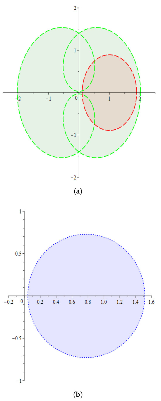
For function $f_1(\zeta )={\displaystyle \frac{\zeta }{1-{\zeta }^2}}=\zeta +{\zeta }^3+{\zeta }^5+\cdots$, it is clear that $f_1$ is analytic and univalent and $f_1\in \mathcal{F}$. A straightforward application of Theorem 7 reports that

$$\Re \left\{{\displaystyle \frac{\zeta {\left({\mathcal{B}}_2^8{f}_1(\zeta )\right)}^{\prime }}{{\mathcal{B}}_2^8{f}_1(\zeta )}}\right\}>0,$$

(58)

since

$${\displaystyle \frac{{\mathcal{B}}_1^8{f}_1(\zeta )}{\zeta }}\prec 1+{\displaystyle \frac{2}{\sqrt{5}}}\zeta .$$

(59)

where

$${\mathcal{B}}_2^8{f}_1(\zeta )=\zeta +\sum _{n=1}^{\infty }{\left({\displaystyle \frac{2^n}{(2n)!}}\right)}^2{\zeta }^{2n+1},$$

(60)

For inequality (58), see Figure 1b. For subordination (59), see Figure 1a.

Taking the restriction $\lambda =1$ in Theorem 7, we state the following corollary:

Corollary 3. 

For $\kappa \ne 1$, $f\in \mathcal{F}$ satisfies

$$\left|{\displaystyle \frac{{\mathcal{B}}_{\kappa -1}^{c}f(\zeta )}{\zeta }}-1\right|<M_1,$$

where

$$M_1={\displaystyle \frac{\xi \eta }{\left|\frac{1-\alpha }{\kappa -1}-1\right|+\sqrt{1+{\left(\frac{\kappa }{\kappa -1}\right)}^2}}}.$$

Then, $f\in S_{\kappa }^c(\alpha )$.

Theorem 8. 

Let $\lambda >0$, $\mu \ge 0$, and $f\in \mathcal{F}$ such that ${\displaystyle \frac{{\mathcal{B}}_{\kappa }^{c}f(\zeta )}{\zeta }}\ne 0$, fulfilling the following subordination:

$$(1-\lambda ){\left({\displaystyle \frac{{\mathcal{B}}_{\kappa }^{c}f(\zeta )}{\zeta }}\right)}^{\mu }+\lambda {({\mathcal{B}}_{\kappa }^{c}f(\zeta ))}^{\prime }{\left({\displaystyle \frac{{\mathcal{B}}_{\kappa }^{c}f(\zeta )}{\zeta }}\right)}^{\mu -1}\prec 1+M_2\zeta ,$$

(61)

where principal values of powers were taken, and

$$M_2=\left\{\begin{array}{cc}\frac{(1-\alpha )\lambda \left(1+\frac{\lambda }{\mu }\right)}{\left|1-(1-\alpha )\lambda \right|+\sqrt{1+{\left(1+\frac{\lambda }{\mu }\right)}^2}}& (\mu >0),\\ & \\ \left(1-\alpha \right)\lambda & (\mu =0).\end{array}\right.$$

Then, $f\in S_{\kappa }^c(\alpha )$.

Proof. 

In the case of $\mu =0$, relation (61) is equivalent to

$$\left|{\displaystyle \frac{\zeta {({\mathcal{B}}_{\kappa }^{c}f(\zeta ))}^{\prime }}{{\mathcal{B}}_{\kappa }^{c}f(\zeta )}}-1\right|<1-\alpha .$$

Consequently, $f\in S_{\kappa }^c(\alpha )$ is implied.

In the case of $\mu >0$, let

$$\varphi (\zeta )={\left({\displaystyle \frac{{\mathcal{B}}_{\kappa }^{c}f(\zeta )}{\zeta }}\right)}^{\mu }.$$

(62)

In (62), select the principle value. Then, we observe that $\varphi$ is analytic in $\left|\zeta \right|<1$. Moreover, $\varphi$ is of the type (14). Additionally, differentiating (62) leads to

$$(1-\lambda ){\left({\displaystyle \frac{{\mathcal{B}}_{\kappa }^{c}f(\zeta )}{\zeta }}\right)}^{\mu }+\lambda {\left({\mathcal{B}}_{\kappa }^{c}f(\zeta )\right)}^{\prime }{\left({\displaystyle \frac{{\mathcal{B}}_{\kappa }^{c}f(\zeta )}{\zeta }}\right)}^{\mu -1}=\varphi (\zeta )+{\displaystyle \frac{\lambda }{\mu }}\zeta {\varphi }^{\prime }(\zeta ).$$

Considering Lemma 1 ($c=\mu /\lambda$), this results in

$$\varphi (\zeta )\prec 1+{\displaystyle \frac{\mu }{\mu +\lambda }}{M}_2\zeta .$$

Furthermore, using (61) and (62), we have

$$\varphi (\zeta )\left[1-\lambda +\lambda (\left(1-\alpha \right)p(\zeta )+\alpha )\right]\prec 1+M_2\zeta ,$$

such that $p(\zeta )$ is expressed in (54). Then, making use of Lemma 3, we arrive at

$$\Re \{p(\zeta )]\}>0,$$

that is,

$$\Re \left\{{\displaystyle \frac{\zeta {({\mathcal{B}}_{\kappa }^{c}f(\zeta ))}^{\prime }}{{\mathcal{B}}_{\kappa }^{c}f(\zeta )}}\right\}>\alpha .$$

The proof of Theorem 8 is therefore finished. □

Taking $\lambda =\mu =1$ within Theorem 8 forms the corollary below.

Corollary 4. 

For $f\in \mathcal{F}$ such that

$$\left|{({\mathcal{B}}_{\kappa }^{c}f(\zeta ))}^{\prime }-1\right|<{\displaystyle \frac{2(1-\alpha )}{\alpha +\sqrt{5}}},$$

(63)

we have $f\in S_{\kappa }^c(\alpha )$.

Theorem 9. 

Suppose that $\mu >0$, $\lambda >0$, and $\nu >-\mu$. If $f\in \mathcal{F}$ holds, the subordination

$$(1-\lambda ){\left({\displaystyle \frac{{\mathcal{B}}_{\kappa }^{c}f(\zeta )}{\zeta }}\right)}^{\mu }+\lambda {({\mathcal{B}}_{\kappa }^{c}f(\zeta ))}^{\prime }{\left({\displaystyle \frac{{\mathcal{B}}_{\kappa }^{c}f(\zeta )}{\zeta }}\right)}^{\mu -1}\prec 1+M_3\zeta ,$$

(64)

such that the powers are the principal ones, and

$$M_3={\displaystyle \frac{(1-\alpha )\lambda \left(1+\frac{\lambda }{\mu }\right)\left(\nu +\mu +1\right)}{\left[\left|1-(1-\alpha )\lambda \right|+\sqrt{1+{\left(1+\frac{\lambda }{\mu }\right)}^2}\right]\left(\nu +\mu \right)}},$$

(65)

Then, $F_{\nu }$ is expressed by

$$F_{\nu }(\zeta ):={\left({\displaystyle \frac{\nu +\mu }{{\zeta }^{\nu }}}{\displaystyle \underset{0}{\overset{\zeta }{\int }}}{t}^{\nu -1}{\left(f(t)\right)}^{\mu }dt\right)}^{1/\mu },$$

(66)

which belongs to $S_{\kappa }^c(\alpha )$.

Proof. 

Clearly, $F_{\nu }\in \mathcal{F}$. Moreover,

$${\zeta }^{\nu }{\left({\mathcal{B}}_{\kappa }^c{F}_{\nu }\left(\zeta \right)\right)}^{\mu }=(\mu +\nu ){\displaystyle \underset{0}{\overset{\zeta }{\int }}}{t}^{\nu -1}{({\mathcal{B}}_{\kappa }^{c}f(t))}^{\mu }dt.$$

(67)

When we differentiate (67), we get

$$(\mu +\nu ){\left({\displaystyle \frac{{\mathcal{B}}_{\kappa }^{c}f(\zeta )}{\zeta }}\right)}^{\mu }=\nu {\left({\displaystyle \frac{{\mathcal{B}}_{\kappa }^c{F}_{\nu }(\zeta )}{\zeta }}\right)}^{\mu }+\mu {({\mathcal{B}}_{\kappa }^c{F}_{\nu }(\zeta ))}^{\prime }{\left({\displaystyle \frac{{\mathcal{B}}_{\kappa }^c{F}_{\nu }(\zeta )}{\zeta }}\right)}^{\mu -1}.$$

(68)

Let

$$\mathcal{G}(\zeta )=(1-\lambda ){\left({\displaystyle \frac{{\mathcal{B}}_{\kappa }^c{F}_{\nu }(\zeta )}{\zeta }}\right)}^{\mu }+\lambda {({\mathcal{B}}_{\kappa }^c{F}_{\nu }(\zeta ))}^{\prime }{\left({\displaystyle \frac{{\mathcal{B}}_{\kappa }^c{F}_{\nu }(\zeta )}{\zeta }}\right)}^{\mu -1},$$

(69)

Then, $\mathcal{G}$ is analytic in $\left|\zeta \right|<1$; also, it takes the type (14). Again, by differentiating (69) and applying (68), we arrive to

$$\mathcal{G}(\zeta )+{\displaystyle \frac{\zeta {\mathcal{G}}^{\prime }(\zeta )}{\mu +\nu }}=(1-\lambda ){\left({\displaystyle \frac{{\mathcal{B}}_{\kappa }^{c}f(\zeta )}{\zeta }}\right)}^{\mu }+\lambda {({\mathcal{B}}_{\kappa }^{c}f(\zeta ))}^{\prime }{\left({\displaystyle \frac{{\mathcal{B}}_{\kappa }^{c}f(\zeta )}{\zeta }}\right)}^{\mu -1}.$$

The aforementioned formula and assumption (64) now indicate that

$$\mathcal{G}(\zeta )+{\displaystyle \frac{\zeta {\mathcal{G}}^{\prime }(\zeta )}{\mu +\nu }}\prec 1+M_3\zeta ,$$

where $M_3$ is given by (65). Now, Lemma 1 gives

$$\mathcal{G}(\zeta )\prec 1+{\displaystyle \frac{\mu +\nu }{\mu +\nu +1}}{M}_3\zeta .$$

(70)

Finally, in applying Theorem 8, if f has been replaced with $F_{\nu }$, then $F_{\nu }\in S_{\kappa }^c(\alpha )$ follows from (70). This finishes the proof. □

Taking $\lambda =\mu =1$ and $\nu =0$ within Theorem 9, the subsequent corollary is obtained.

Corollary 5. 

Let $f\in \mathcal{F}$ fulfill the subordination

$$\left|{({\mathcal{B}}_{\kappa }^{c}f(\zeta ))}^{\prime }-1\right|<{\displaystyle \frac{4(1-\alpha )}{\alpha +\sqrt{5}}},$$

(71)

Then,

$${\displaystyle {\int }_0^{\zeta }}{\displaystyle \frac{f(t)}{t}}dt\in S_{\kappa }^c(\alpha ).$$

Theorem 10. 

If the functions ${\displaystyle \frac{{\mathcal{B}}_{\kappa -1}^c{f}_j(\zeta )}{\zeta }}\in P\left({\gamma }_j\right)({\gamma }_j={\displaystyle \frac{1-C_j}{1-D_j}},-1\le D_j<C_j\le 1,f_j\in \mathcal{F};j=1,2)$, then $\mathfrak{h}$, defined by

$$\mathfrak{h}(\zeta )={\mathcal{B}}_{\kappa }^c\left(f_1\ast f_2\right)(\zeta ),$$

(72)

satisfies

$$\Re \left\{{\displaystyle \frac{{\mathcal{B}}_{\kappa -1}^c\mathfrak{h}(\zeta )}{{\mathcal{B}}_{\kappa }^c\mathfrak{h}(\zeta )}}\right\}>0(\zeta \in ▿),$$

(73)

provided that

$${\displaystyle \frac{\left(C_1-D_1\right)\left(C_2-D_2\right)}{\left(1-D_1\right)\left(1-D_2\right)}}\le {\displaystyle \frac{2\kappa -1}{2\left[{\left({}_{2}F_1\left(1,1;\kappa ;\frac{1}{2}\right)-2\right)}^2+2(\kappa -1)\right]}}.$$

(74)

Proof. 

We have ${\displaystyle \frac{{\mathcal{B}}_{\kappa -1}^c{f}_j(\zeta )}{\zeta }}\in P\left({\gamma }_j\right)({\gamma }_j={\displaystyle \frac{1-C_j}{1-D_j}};j=1,2)$.

Therefore, we can determine from Lemma 5 that

$$\Re \left\{{\displaystyle \frac{{\mathcal{B}}_{\kappa -1}^c{f}_1(\zeta )}{\zeta }}\ast {\displaystyle \frac{{\mathcal{B}}_{\kappa -1}^c{f}_2(\zeta )}{\zeta }}\right\}>1-2{\displaystyle \frac{\left(C_1-D_1\right)\left(C_2-D_2\right)}{\left(1-D_1\right)\left(1-D_2\right)}}.$$

Using $\mathfrak{h}(\zeta )={\mathcal{B}}_{\kappa }^c{f}_0(\zeta );$ $f_0(\zeta )=\left(f_1\ast f_2\right)(\zeta )$, (7) makes it simple to demonstrate that

$$\begin{array}{cc}\hfill {\displaystyle \frac{{\mathcal{B}}_{\kappa -1}^c{f}_1(\zeta )}{\zeta }}\ast {\displaystyle \frac{{\mathcal{B}}_{\kappa -1}^c{f}_2(\zeta )}{\zeta }}& ={\displaystyle \frac{1}{\zeta }}{\mathcal{B}}_{\kappa -1}^c\left({\mathcal{B}}_{\kappa -1}^c{f}_0(\zeta )\right)\hfill \\ \hfill & =\frac{1}{\zeta }{\mathcal{B}}_{\kappa -1}^c\left(\frac{1}{\kappa -1}\left[(\kappa -2){\mathcal{B}}_{\kappa }^c{f}_0(\zeta )+\zeta {\left({\mathcal{B}}_{\kappa }^c{f}_0(\zeta )\right)}^{\prime }\right]\right)\hfill \\ \hfill & =\frac{1}{\zeta }\frac{1}{\kappa -1}\left[(\kappa -2){\mathcal{B}}_{\kappa -1}^c\left({\mathcal{B}}_{\kappa }^c{f}_0(\zeta )\right)+\zeta {\left({\mathcal{B}}_{\kappa -1}^c\left({\mathcal{B}}_{\kappa }^c{f}_0(\zeta )\right)\right)}^{\prime }\right]\hfill \\ \hfill & ={\displaystyle \frac{\kappa -2}{\kappa -1}}{\displaystyle \frac{{\mathcal{B}}_{\kappa -1}^c\mathfrak{h}(\zeta )}{\zeta }}+{\displaystyle \frac{1}{\kappa -1}}{\left({\mathcal{B}}_{\kappa -1}^c\mathfrak{h}(\zeta )\right)}^{\prime }\hfill \\ \hfill & ={\displaystyle \frac{{\mathcal{B}}_{\kappa -1}^c\mathfrak{h}(\zeta )}{\zeta }}+{\displaystyle \frac{\zeta }{\kappa -1}}{\left({\displaystyle \frac{{\mathcal{B}}_{\kappa -1}^c\mathfrak{h}(\zeta )}{\zeta }}\right)}^{\prime }.\hfill \end{array}$$

Thus,

$$\Re \left\{{\displaystyle \frac{{\mathcal{B}}_{\kappa -1}^c\mathfrak{h}(\zeta )}{\zeta }}+{\displaystyle \frac{\zeta }{\kappa -1}}{\left({\displaystyle \frac{{\mathcal{B}}_{\kappa -1}^c\mathfrak{h}(\zeta )}{\zeta }}\right)}^{\prime }\right\}>1-2{\displaystyle \frac{\left(C_1-D_1\right)\left(C_2-D_2\right)}{\left(1-D_1\right)\left(1-D_2\right)}},$$

(75)

Applying Lemma 1 to the case of

$$\delta =\kappa -1,C=-1+4{\displaystyle \frac{\left(C_1-D_1\right)\left(C_2-D_2\right)}{\left(1-D_1\right)\left(1-D_2\right)}}\mathrm{and}D=-1,$$

leads to

$$\Re \left\{{\displaystyle \frac{{\mathcal{B}}_{\kappa -1}^c\mathfrak{h}(\zeta )}{\zeta }}\right\}>1+\frac{\left(C_1-D_1\right)\left(C_2-D_2\right)}{\left(1-D_1\right)\left(1-D_2\right)}\left[{}_{2}F_1\left(1,1;\kappa ;{\displaystyle \frac{1}{2}}\right)-2\right](\zeta \in ▿).$$

(76)

Using inequality (76) together with Theorem 2 for $\lambda =\sigma =1$,

$$C=-1-4{\displaystyle \frac{\left(C_1-D_1\right)\left(C_2-D_2\right)}{\left(1-D_1\right)\left(1-D_2\right)}}\left[{}_{2}F_1\left(1,1;\kappa ;{\displaystyle \frac{1}{2}}\right)-2\right],$$

and $D=-1$, we conclude that

$$\Re \left\{\theta (\zeta )\right\}>1-2{\displaystyle \frac{\left(C_1-D_1\right)\left(C_2-D_2\right)}{\left(1-D_1\right)\left(1-D_2\right)}}{\left[{}_{2}F_1\left(1,1;\kappa ;{\displaystyle \frac{1}{2}}\right)-2\right]}^2(\zeta \in ▿),$$

(77)

where $\theta (\zeta )={\mathcal{B}}_{\kappa -1}^c\mathfrak{h}(\zeta )/\zeta$. If we set

$$\mathsf{\Omega }(\zeta )={\displaystyle \frac{{\mathcal{B}}_{\kappa -1}^c\mathfrak{h}(\zeta )}{{\mathcal{B}}_{\kappa }^c\mathfrak{h}(\zeta )}}(\zeta \in ▿),$$

then $\mathsf{\Omega }$ is analytic; also, it takes formula (14). Some calculations can give that

$$\begin{array}{cc}\hfill {\displaystyle \frac{{\mathcal{B}}_{\kappa -1}^c\mathfrak{h}(\zeta )}{\zeta }}+{\displaystyle \frac{\zeta }{\kappa -1}}{\left({\displaystyle \frac{{\mathcal{B}}_{\kappa -1}^c\mathfrak{h}(\zeta )}{\zeta }}\right)}^{\prime }& =\theta (\zeta )\left[{\left(\mathsf{\Omega }(\zeta )\right)}^2+{\displaystyle \frac{\zeta }{\kappa -1}}{\mathsf{\Omega }}^{\prime }(\zeta )\right]\hfill \\ \hfill & =\mathsf{\Psi }\left(\mathsf{\Omega }(\zeta ),\zeta {\mathsf{\Omega }}^{\prime }(\zeta );\zeta \right),\hfill \end{array}$$

(78)

where $\mathsf{\Psi }\left(u,v;\zeta \right)=\theta (\zeta )\left(u^2+{\displaystyle \frac{v}{\kappa -1}}\right)$. Thus, using (75) in (78), we deduce that

$$\Re \left\{\mathsf{\Psi }\left(\mathsf{\Omega }(\zeta ),\zeta {\mathsf{\Omega }}^{\prime }(\zeta );\zeta \right)\right\}>1-2{\displaystyle \frac{\left(C_1-D_1\right)\left(C_2-D_2\right)}{\left(1-D_1\right)\left(1-D_2\right)}}(\zeta \in ▿).$$

The real $x,y\le -\left(x^2+1\right)/2$ give

$$\begin{array}{cc}\hfill \Re \left\{\mathsf{\Psi }\left(ix,y;\zeta \right)\right\}& =\left({\displaystyle \frac{y}{\kappa -1}}-x^2\right)\Re \left\{\theta (\zeta )\right\}\hfill \\ \hfill & \le -{\displaystyle \frac{1}{2\left(\kappa -1\right)}}\left[1+\left(2\left(\kappa -1\right)+1\right)x^2\right]\Re \left\{\theta (\zeta )\right\}\hfill \\ \hfill & \le {\displaystyle \frac{\Re \left\{\theta (\zeta )\right\}}{2\left(\kappa -1\right)}}\le 1-2{\displaystyle \frac{\left(C_1-D_1\right)\left(C_2-D_2\right)}{\left(1-D_1\right)\left(1-D_2\right)}}(\zeta \in ▿),\hfill \end{array}$$

by (74) and (77). Consequently, we obtain $\Re \left\{\mathsf{\Omega }(\zeta )\right\}>0(\zeta \in ▿)$ by applying Lemma 2. The proof is complete. □

Theorem 11. 

If ${\displaystyle \frac{{\mathcal{B}}_{\kappa -1}^c{f}_j(\zeta )}{\zeta }}\in P\left({\gamma }_j\right)({\gamma }_j={\displaystyle \frac{1-C_j}{1-D_j}},-1\le D_j<C_j\le 1,f_j\in \mathcal{F};j=1,2,3)$, then $\mathfrak{H}(\zeta )={\mathcal{B}}_{\kappa }^c\left(f_1\ast f_2\ast f_3\right)(\zeta )$ satisfies

$$\Re \left\{{\displaystyle \frac{{\mathcal{B}}_{2\kappa -2}^c\mathfrak{H}(\zeta )}{{\mathcal{B}}_{2\kappa -1}^c\mathfrak{H}(\zeta )}}\right\}>0(\zeta \in ▿),$$

(79)

provided that

$${\displaystyle \frac{\left(C_1-D_1\right)\left(C_2-D_2\right)\left(C_3-D_3\right)}{\left(1-D_1\right)\left(1-D_2\right)\left(1-D_3\right)}}<{\displaystyle \frac{2\kappa -1}{4\left[{\left({}_{2}F_1\left(1,1;\kappa ;\frac{1}{2}\right)-2\right)}^2+2(\kappa -1)\right]}}.$$

(80)

Proof. 

Using (72), it is easy to verify that

$$\begin{array}{cc}\hfill \Re \left\{{\displaystyle \frac{{\mathcal{B}}_{2\kappa -2}^c\mathfrak{h}(\zeta )}{\zeta }}+{\displaystyle \frac{\zeta }{\kappa -1}}{\left({\displaystyle \frac{{\mathcal{B}}_{2\kappa -2}^c\mathfrak{h}(\zeta )}{\zeta }}\right)}^{\prime }\right\}& =\Re \left\{{\displaystyle \frac{{\mathcal{B}}_{\kappa -1}^c{f}_1(\zeta )}{\zeta }}\ast {\displaystyle \frac{{\mathcal{B}}_{\kappa -1}^c{f}_2(\zeta )}{\zeta }}\ast {\displaystyle \frac{{\mathcal{B}}_{\kappa -1}^c{f}_3(\zeta )}{\zeta }}\right\}\hfill \\ \hfill & >{\displaystyle \frac{2\kappa -1}{4\left[{\left({}_{2}F_1\left(1,1;\kappa ;\frac{1}{2}\right)-2\right)}^2+2(\kappa -1)\right]}}(\zeta \in ▿),\hfill \end{array}$$

and we skip the details since the proof of Theorem 11 can be finished in a way similar to that of Theorem 10. □

Theorem 12. 

For $j\in \{1,2\}$, let $f_j\in \mathcal{F}$. Additionally, for $\mathfrak{h}$ expressed in (72), it satisfies

$$\Re \left\{{\displaystyle \frac{{\mathcal{B}}_{\kappa -1}^c\mathfrak{h}(\zeta )}{\zeta }}\right\}>1-{\displaystyle \frac{2\kappa -1}{2\left[{\left({}_{2}F_1\left(1,1;\kappa ;\frac{1}{2}\right)-2\right)}^2+2\left(\kappa -1\right)\right]}}(\zeta \in ▿),$$

Then,

$$\Re \left\{{\displaystyle \frac{{\mathcal{B}}_{\kappa -1}^c\mathfrak{G}(\zeta )}{{\mathcal{B}}_{\kappa }^c\mathfrak{G}(\zeta )}}\right\}>0(\zeta \in ▿),$$

where

$$\mathfrak{G}(\zeta )={\displaystyle \frac{\kappa -1}{{\zeta }^{\kappa -2}}}\underset{0}{\overset{\zeta }{\int }}{t}^{\kappa -3}\mathfrak{h}(t)dt(\zeta \in ▿).$$

Proof. 

Use the following inequality:

$$\begin{array}{cc}\hfill \Re \left\{{\displaystyle \frac{{\mathcal{B}}_{\kappa -1}^c\mathfrak{G}(\zeta )}{\zeta }}+{\displaystyle \frac{\zeta }{\kappa -1}}{\left({\displaystyle \frac{{\mathcal{B}}_{\kappa -1}^c\mathfrak{G}(\zeta )}{\zeta }}\right)}^{\prime }\right\}& =\Re \left\{{\displaystyle \frac{{\mathcal{B}}_{\kappa -1}^c\mathfrak{h}(\zeta )}{\zeta }}\right\}\hfill \\ \hfill & >1-{\displaystyle \frac{2\kappa -1}{2\left[{\left({}_{2}F_1\left(1,1;\kappa ;\frac{1}{2}\right)-2\right)}^2+2\left(\kappa -1\right)\right]}}(\zeta \in ▿).\hfill \end{array}$$

At this stage, the proof can be completed, and the details are left out. □

6. Conclusions

The Bessel function is one of the most significant special functions. A generalized version of this function was utilized in this article. This extended Bessel function yields new results as well as direct implications for some modified versions of the ordinary Bessel function, of which there are three forms (modified, spherical, and ordinary). Based on this role of the generalized function, we drew upon previous studies and applied them to obtain the operator ${\mathcal{B}}_{\kappa }^c$ on a class of analytic functions defined on the unit disk. This class also generalizes well-known classes of functions in the field of Geometric Function Theory of complex variables by employing the principle of differential subordination and the concept of convolution of functions. The operator ${\mathcal{B}}_{\kappa }^c$ generalizes the other existing operator by specializing parameters $\kappa$ and c. Additionally, we looked into some sufficient starlike requirements and assessments for a particular subset of univalent functions in ▿. By specializing the parameters in all theorems obtained here, we will be able to determine the consequences of ${\mathcal{N}}_{\kappa }$, ${\mathcal{J}}_p$, ${\mathcal{I}}_p$, and ${\mathcal{S}}_p$ as special cases of ${\mathcal{B}}_{\kappa }^c$. For further studies, we recommend investigations to be conducted on the Mittag–Leffler function [34], Hurwitz–Lerch Zeta function [35], Dini [36] and Einstein [37,38] functions, etc.

References

- Baricz, Á. Generalized Bessel Functions of the First Kind; Lecture Notes in Mathematics; Springer: Berlin/Heidelberg, Germany, 2010; Volume 1994. [Google Scholar]
- Watson, G.N. A Treatise on the Theory of Bessel Functions, 2nd ed.; Cambridge University Press: Cambridge, UK; London, UK; New York, NY, USA, 1944. [Google Scholar]
- Deniz, E. Convexity of integral operators involving generalized Bessel functions. Integral Transform. Spec. Funct. 2013, 24, 201–216. [Google Scholar] [CrossRef]
- Deniz, E.; Orhan, H.; Srivastava, H.M. Some sufficient conditions for univalence of certain families of integral operators involving generalized Bessel functions. Taiwan. J. Math. 2011, 15, 883–917. [Google Scholar] [CrossRef]
- Baricz, Á. Some inequalities involving generalized Bessel functions. Math. Inequal. Appl. 2007, 10, 827–842. [Google Scholar] [CrossRef]
- Baricz, Á. Geometric properties of generalized Bessel functions. Publ. Math. Debr. 2008, 73, 155–178. [Google Scholar] [CrossRef]
- Baricz, Á.; Frasin, B.A. Univalence of integral operators involving Bessel functions. Appl. Math. Lett. 2010, 23, 371–376. [Google Scholar] [CrossRef]
- Baricz, Á.; Ponnusamy, S. Starlikeness and convexity of generalized Bessel functions. Integral Transform. Spec. Funct. 2010, 21, 641–653. [Google Scholar] [CrossRef]
- Frasin, B.A. Sufficient conditions for integral operator defined by Bessel functions. J. Math. Inequal. 2010, 4, 301–306. [Google Scholar] [CrossRef]
- Balasubramanian, R.; Ponnusamy, S.; Prabhakaran, D.J. Convexity of integral transforms and function spaces. Integral Transform. Spec. Funct. 2007, 18, 1–14. [Google Scholar] [CrossRef]
- Breaz, D. A convexity property for an integral operator on the class, Sα(β). Gen. Math. 2007, 15, 177–183. [Google Scholar]
- Breaz, N.; Breaz, D.; Darus, M. Convexity properties for some general integral operators on uniformly analytic functions classes. Comput. Math. Appl. 2010, 60, 3105–3107. [Google Scholar] [CrossRef][Green Version]
- Breaz, D.; Breaz, N.; Srivastava, H.M. An extension of the univalent condition for a family of integral operators. Appl. Math. Lett. 2009, 22, 41–44. [Google Scholar] [CrossRef]
- Breaz, D.; Güney, H. The integral operator on the classes, and Cα(β). J. Math. Inequal. 2008, 2, 97–100. [Google Scholar] [CrossRef]
- Frasin, B.A. Some sufficient conditions for certain integral operators. J. Math. Inequal. 2008, 2, 527–535. [Google Scholar] [CrossRef]
- Macarie, V.M.; Breaz, D. The order of convexity of some general integral operators. Comput. Math. Appl. 2011, 62, 4667–4673. [Google Scholar] [CrossRef][Green Version]
- Ponnusamy, S.; Singh, V.; Vasundhra, P. Starlikeness and convexity of an integral transform. Integral Transform. Spec. Funct. 2004, 15, 267–280. [Google Scholar] [CrossRef]
- Srivastava, H.M.; Deniz, E.; Orhan, H. Some general univalence criteria for a family of integral operators. Appl. Math. Comput. 2010, 215, 3696–3701. [Google Scholar] [CrossRef]
- Kershaw, J.; Obata, T. Computing the zeros of cross-product combinations of the Bessel functions with complex order. Results Appl. Math. 2025, 28, 100642. [Google Scholar] [CrossRef]
- Kumaria, N.; Prajapata, J.K. Improved geometric properties of unified Struve function. Filomat 2025, 39, 6199–6214. [Google Scholar]
- Özkan, Y.; Deniz, E.; Kazimoğlu, S. Radii of starlikeness and convexity of extended generalized k-Bessel functions. J. Anal. 2025. [Google Scholar] [CrossRef]
- Taşar, N.; Sakar, F.M.; Frasin, B.; Aldawish, I. Categories of harmonic functions in the symmetric unit disk linked to the Bessel function. Symmetry 2025, 17, 1581. [Google Scholar] [CrossRef]
- Tyr, O.; Dades, A. Several theorems of approximation theory for the q-bessel transform. Kragujev. J. Math. 2027, 51, 237–250. [Google Scholar]
- Miller, S.S.; Mocanu, P.T. Differential Subordinations and univalent functions. Mich. Math. J. 1981, 28, 157–171. [Google Scholar] [CrossRef]
- Miller, S.S.; Mocanu, P.T. Differential Subordinations: Theory and Applications; Series on Monographs and Textbooks in Pure and Appl. Math. No. 255; Marcel Dekker, Inc.: New York, NY, USA, 2000. [Google Scholar]
- Liu, M.-S. On certain sufficient condition for starlike functions. Soochow J. Math. 2003, 29, 407–412. [Google Scholar]
- Pashkouleva, D.Z. The starlikeness and spiral-convexity of certain subclasses of analytic. In Current Topics in Analytic Function Theory; Srivastava, H.M., Owa, S., Eds.; World Scientific Publishing Company: Singapore; Hackensack, NJ, USA; London, UK; Hong Kong, China, 1992. [Google Scholar]
- Stankiewicz, J.; Stankiewicz, Z. Some applications of the Hadamard convolution in the theory of functions. Ann. Univ. Mariae Curie-Sklodwska Sect. A 1986, 40, 251–265. [Google Scholar]
- Whittaker, E.T.; Watson, G.N. A Course on Modern Analysis: An Introduction to the General Theory of Infinite Processes and of Analytic Functions with an Account of the Principal Transcendental Functions, 4th ed.; Cambridge University Press: Cambridge, UK, 1927. [Google Scholar]
- Owa, S.; Srivastava, H.M. Some applications of the generalized Libera integral operator. Proc. Japan Acad. Ser. A Math. Sci. 1986, 62, 125–128. [Google Scholar] [CrossRef]
- Ruscheweyh, S.; Sheil-Small, T. Hadamard products of schlicht functions and the poloya-schoenberg conjecture. Comment. Math. Helv. 1973, 48, 119–135. [Google Scholar] [CrossRef]
- Nehari, Z. Conformal Mapping; MaGraw-Hill: New York, NY, USA, 1952. [Google Scholar]
- Janowski, W. Extremal problems for a family of functions with positive real part and some related families. Ann. Polon. Math. 1970, 23, 159–177. [Google Scholar] [CrossRef]
- Ali, E.E.; El-Ashwah, R.M.; Kota, W.Y.; Albalahi, A.M. Geometric attributes of analytic functions generated by Mittag-Leffler function. Mathematics 2025, 13, 3284. [Google Scholar] [CrossRef]
- Ali, E.E.; El-Ashwah, R.M.; Albalahi, A.M.; Sidaoui, R. Fuzzy treatment for meromorphic classes of admissible functions connected to Hurwitz–Lerch zeta function. Axioms 2025, 14, 523. [Google Scholar] [CrossRef]
- El-Qadeem, A.H.; Mamon, M.A.; Elshazly, I.S. On the partial sums of the q-generalized Dini function. J. Math. 2022, 2022, 8496249. [Google Scholar] [CrossRef]
- El-Qadeem, A.H.; Murugusundaramoorthy, G.; Halouani, B.; Elshazly, I.S.; Vijaya, K.; Mamon, M.A. On λ-pseudo bi-starlike functions related to second Einstein function. Symmetry 2024, 16, 1429. [Google Scholar] [CrossRef]
- El-Qadeem, A.H.; Saleh, S.A.; Mamon, M.A. Bi-univalent function classes defined by using a second Einstein function. J. Funct. Spaces 2022, 2022, 6933153. [Google Scholar] [CrossRef]
Disclaimer/Publisher’s Note: The statements, opinions and data contained in all publications are solely those of the individual author(s) and contributor(s) and not of MDPI and/or the editor(s). MDPI and/or the editor(s) disclaim responsibility for any injury to people or property resulting from any ideas, methods, instructions or products referred to in the content. |
© 2025 by the authors. Licensee MDPI, Basel, Switzerland. This article is an open access article distributed under the terms and conditions of the Creative Commons Attribution (CC BY) license (https://creativecommons.org/licenses/by/4.0/).