Article

A Methodological Framework for Analyzing and Differentiating Daily Physical Activity Across Groups Using Digital Biomarkers from the Frequency Domain

1
Institute of Epidemiology and Preventive Medicine, College of Public Health, National Taiwan University, Taipei 100025, Taiwan
2
Institute of Health Data Analytics and Statistics, College of Public Health, National Taiwan University, Taipei 100025, Taiwan
3
Master of Public Health Program, College of Public Health, National Taiwan University, Taipei 100025, Taiwan
4
Bioinformatics and Biostatistics Core Lab, Centers of Genomic and Precision Medicine, National Taiwan University, Taipei 100025, Taiwan
5
Department of Public Health, College of Public Health, National Taiwan University, Taipei 100025, Taiwan
*
Author to whom correspondence should be addressed.
Mathematics 2025, 13(22), 3616; https://doi.org/10.3390/math13223616
Submission received: 18 September 2025 / Revised: 3 November 2025 / Accepted: 7 November 2025 / Published: 11 November 2025
(This article belongs to the Special Issue Advanced Methods and Applications in Medical Informatics)

Abstract

Human daily physical activity (PA), monitored via wearable devices, provides valuable information for real-time health assessment and disease prevention. However, analyzing time-domain PA data is challenging due to large data volumes and high inter- and intra-individual heterogeneity. Traditional PA analyses often rely on demographics, while advanced methods utilize time-domain summary statistics (e.g., L5, M10) or functional principal component analysis (FPCA). This study presents a data-efficient approach utilizing the Discrete Fourier Transform (DFT) to convert time-domain data into a compact set of frequency-domain variables. Our research suggests that adding these DFT variables can significantly enhance model performance. We demonstrate that incorporating DFT-derived variables substantially improves model performance. Specifically, (1) a small subset of DFT variables effectively captures major PA levels with effective dimensionality reduction; (2) these variables retain known associations with factors like age, sex, and weekday/weekend status; (3) they enhance the performance of classifiers. Mathematical and empirical analyses further confirm the reliability and interpretability of DFT-based features in dimension reduction. Across three mental health studies, these DFT-derived variables successfully capture key PA characteristics while retaining known associations and strengthening model performance. Overall, the proposed DFT-based framework offers a robust and scalable tool for analyzing accelerometer data, with broad applicability in health and behavioral research.

1. Introduction

The technological revolution has had a profound impact on the variety and volume of data being collected. This is particularly evident with the rise of wearables and the digital data they generate. With the built-in sensors, individuals’ physical movements, distance traveled, and geographical positions can be recorded and documented in milliseconds or shorter intervals [1,2,3,4]. The resulting data provide personalized, free-living, and dynamic information, enabling the monitoring of real-time activities related to human health, including depression status, cardiac rehabilitation, obesity, sleep behavior, and mortality [3,4,5,6,7]. Wearable devices were also employed in micro-randomized intervention trials to assess the effects of interventions on health behaviors [8,9,10]. Modeling and analysis of the digital data, however, are not straightforward, and challenges arise. For instance, in the prospective UK Biobank (UKB) study, the free-living physical activity (PA) of approximately 100,000 participants was monitored using a triaxial accelerometer at 100 Hz per second for seven consecutive days [11], resulting in a dataset of enormous volume. The preprocessing procedures and analysis for such high-volume time series data can be computationally costly. The second challenge relates to the choice of activity metrics. Common measures are activity count (AC), activity index (AI), Euclidean Norm Minus One (ENMO), and angle-Z [12,13,14]. Among the existing activity measures, no single measure has demonstrated consistent superiority over the others [12,13]. Studies reported that, for moderate and vigorous physical activities, ENMO and AI are more sensitive [12], while angle-Z is more reliable in estimating sleep period time windows [14]. These metrics are often available from the commercial software provided by the device manufacturer or can be calculated with free online packages, such as ActivityIndex [12] and GGIR package in R (Version 4.0.4) [15]. In the following descriptions, we use the terminology activity level to represent the various PA metrics in general. Furthermore, difficulties in methodology development arise when model construction and feature extraction for PA are of interest, especially when each participant is monitored over multiple days, due to high heterogeneity both within and between individuals [16,17]. This may blur differences when comparing mean activity and incur a loss in statistical power.

1.1. PA Variables in the Time Domain

To address the challenge of high data volume, existing tools often rely on summary statistics such as the mean, median, or variance of activity levels across fixed time intervals. These intervals can be a day, the most active 10 h (M10) [18], the least active 5 h (L5) [18], or the sleep period time (SPT) window. Additional summary statistics like IV (intra-day variability) and IS (inter-day stability) are also used [18]. These metrics can be incorporated into regression or machine learning models for effect association or classification studies [17,19,20]. While these metrics are intuitive and easy to calculate, they do not capture patterns within the considered time intervals. To address the heterogeneity, the Generalized Linear Mixed-effect Model (GLMM) with random effects to account for the heterogeneity across individuals and the inherent correlation among repeated measurements was proposed [19,21] but was not designed to analyze random PA functions per person per day.

1.2. PA Variables in Frequency Domain

In contrast to the analyses with variables in the time domain, a different approach is to examine the activity level from the perspective of the frequency domain using the Discrete Fourier Transform. The transformation is computed efficiently using the Fast Fourier Transform (FFT) algorithm.
Traditionally, analyses of PA data have been conducted in the time domain, where PA time-series data are reduced to summary statistics (such as L5/M10) and then used as independent variables in classification or association models. However, while time-domain analyses often rely on these summary statistics, which sacrifice meaningful temporal patterns and within-day variability, the DFT offers a systematic solution to the challenge of high-dimensionality in time-series data [22]. The DFT converts the complex time-domain signal into a sparse frequency-domain representation, making it a well-established transformation technique for dimensionality reduction [23]. This methodological choice is further supported by the physiological nature of PA signals: existing literature demonstrates that the majority of signal power and the high-amplitude peaks relevant to activity are concentrated within the low-frequency spectrum, typically between 0 and 15 Hz [23].
The DFT is a useful tool in signal processing that captures cyclic patterns and filters noise in data collected through time [24]. The DFT transforms the temporal data in the time domain into the frequency domain, producing a combination of sinusoid functions to represent the underlying characteristics of the original activity level x m j t observed at discrete time t ( t = 0 , , T 1 ) for the m -th individual on the j -th day.
X m j F k = t = 0 T 1 x m j t e 2 i π T k t , k = 0 , , T 1
Each of the T transformed periodic quantities, X m j F ( k ) , for k = 0 , , T 1 , is a summation of sinusoid functions (the complex exponentials), denoting the component frequency k with absolute value | | X m j F k | | being the amplitude in the same unit as the original x m j t , say gravity g. Now, in the frequency domain, the activity level is reparameterized as functions. Each temporal function is characterized by its amplitude and frequency, representing the strength of the activity level and the occurrence rate of such activity, respectively. Several studies have analyzed this type of variable, including the mean amplitude deviation, maximum amplitude, and the relative amplitude of most and least active hours [20,25]; however, its application remains limited. Note that the i in the complex exponentials in Equation (1) represents the imaginary number, not the index for individuals. It is retained if it does not cause confusion.
In summary, this research addresses the significant analytical challenges posed by the high volume, high dimensionality, and subject-specific heterogeneity of physical activity data from wearable sensors, which traditional time-domain analyses and simple summary statistics inherently fail to capture effectively. Therefore, this study proposes the DFT-based feature extraction framework as a strategic and robust methodological alternative. By employing the DFT to convert the complex time-series data into a sparse frequency-domain representation, the approach achieves substantial dimensionality and computational reduction. Furthermore, leveraging the physiological principle that meaningful PA information, such as daily and weekly rhythms, is concentrated within the low-frequency spectrum, our approach provides enhanced interpretability and offers an effective strategy for handling large-scale, high-frequency wearable datasets by isolating fundamental activity rhythms as novel “digital phenotypes” for use in subsequent statistical and machine learning models.
The objectives of this research are threefold. Firstly, we aim to demonstrate the effectiveness of DFT and inverse DFT (IDFT) in capturing major activity levels using a reduced set of the DFT digital variables. Secondly, these DFT-based variables in the reduced set are evaluated for weekday/weekend, age, sex, and group effects, to examine if these known effects can be retained in the DFT variables. Lastly, we demonstrate the use of these components as features in machine learning models and highlight the improvement in classification performance across three studies, with sample sizes ranging from fewer than 100 to over 20,000.

2. Materials and Methods

2.1. Motivating Studies and Physical Activity Observations

The motivating examples included the probable mental status of individuals in UKB study [26], and two clinical mental studies Depresjon [27] and Psykose [28] (see Appendix A.1 for detailed dataset descriptions). Each study contained 21,007, 54, and 55 participants, respectively. In the UKB study, each participant’s mental status was classified as probable bipolar (PrBP), probable major depression (PrMDD) [26]. The individuals were diagnosed with depression or not in Depresjon and schizophrenia or not in the Psykose study. These individuals wore Axivity Ax3 (100 Hz) or Actiwatch AW4 (32 Hz) wearables for multiple days, and the ENMO or the Activity Count was used as the metric of physical activity level. Figure 1 outlines the rigorous multi-stage data filtration process applied to each cohort, distinguishing between participant-level exclusions in Panel A (UKB) and day-level exclusions in Panels B and C (Depresjon and Psykose).
Note that the PA levels were different for different wearables. In the UKB, the accelerometry value was recorded 8.64 million times daily, and the five-second median filtered ENMO was calculated. It ranged from 0 to 8 g, and the total recorded daily activity levels were 17,280. In the other two studies, the Activity Count was generated by Actiwatch at 32 Hz and scaled by accelerations per minute, leading to a total of 1440 points per day. Each count was a one-minute total activity count ranging between 0 and 3000. To maintain similar amplitude values, the collected activity counts were divided by 1000 before analysis. Table 1 highlights the basic descriptions, and more details can be found in Supplementary Tables S1–S3.
This research was approved by the National Taiwan University Research Ethics Committee, and the reference numbers are 202104HM025 and 202404HM018. Consent forms from subjects to participate in this research are not applicable because the data analyzed here are anonymous, de-linked, and downloaded from the UK Biobank data portal https://www.ukbiobank.ac.uk/ (accessed on 20 March 2024) with applications, from http://datasets.simula.no/depresjon/ (accessed on 1 June 2025) for the Depresjon study data and from https://datasets.simula.no/psykose/ (accessed on 1 June 2025) for the Psykose study data.

2.2. Properties of Frequency Domain Variables

Based on Equation (1), the DFT representation variables, X m j F 0 , X m j F 1 , , X m j F T 1 , in each study can be obtained using the FFT algorithm function fft available in the R software. Here T is the number of time points in a day at which the acceleration values were documented. For instance, in the UKB study, the T was 17,280 per day; while in the Depresjon and Psykose studies, it was 1440 per day.
Three properties of the DFT variables are worth mentioning. First, the component wave with frequency 0, X m j F 0 , represents the total activity over T time points within a day. It can be viewed as a summary statistic of the activity level. Second, the low-frequency waves often represent unique or prominent patterns in a day, with corresponding amplitudes denoting the strength of these special patterns. In contrast, waves with high frequencies represent activities repeating more often than those with low frequencies. In addition, waves of extremely large frequencies may indicate common variations, often referred to as large-frequency noise. Third, the waves X m j F 1 , , X m j F T 1 are symmetric. In other words, the amplitude | | X m j F k | | is the same as | | X m j F T k | | with k between 1 and the integer value of T / 2 . This implies that one only needs to record half of the T periodic waves, which is a great advantage when handling a large amount of data.

2.3. Approximate Activity Curve and Dimension Reduction

Since the daily activity level is now decomposed into T periodic waves, each of these constituents provides partial information through the corresponding frequency k and amplitude A m j k where A m j k = X m j F ( k ) . A partial set S containing p % from these T waves can be applied with the IDFT to approximate the original activity curve to further alleviate the curse of dimensionality (see theoretical justification in Appendix B). It is intuitive to include the first few low-frequency waves in the set, as they represent major daily activity motions, along with the high-frequency waves that are symmetric to them, capturing random variations. The estimated PA at any time t based on the IDFT is then.
x ^ m j ( t ) = 1 T k S X m j F k e 2 i π T k t , t = 0 , , T 1
Here x ^ m j ( t ) denotes the approximation of x m j ( t ) . Note that the summation is still divided by T because waves outside S are replaced with null.
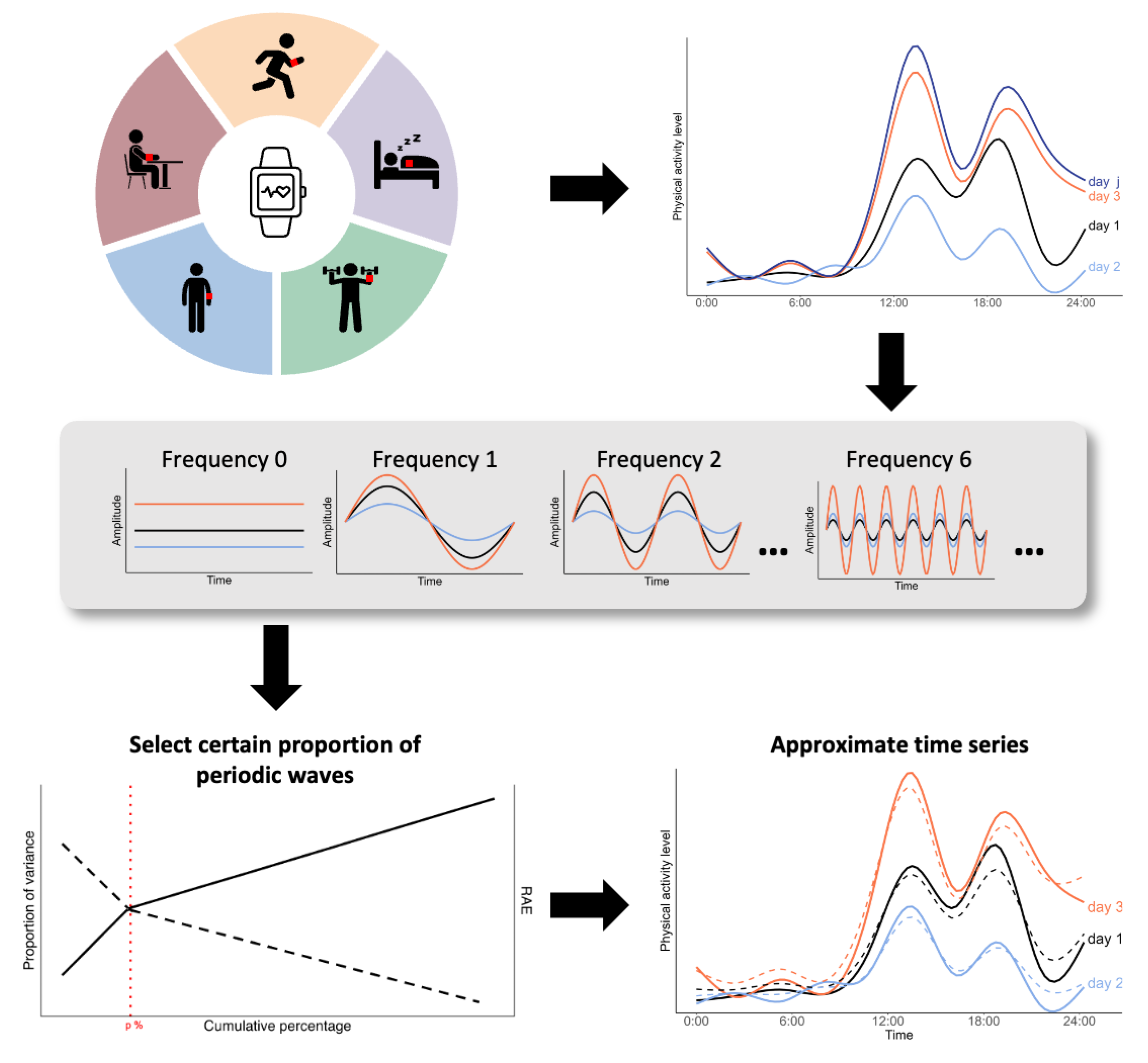
The approximation is guaranteed since it is known that the partial sum of the Fourier series can converge to its original function in L 2 [29], and a quantitative bound on the error for smooth signals is provided in Appendix B. Therefore, the sum in Equation (2), if starting from the leading terms, will approximate well the original PA curve. To investigate how large the set should be, we evaluate its corresponding performance of approximation by the relative absolute error (RAE), Pearson correlation, and proportion of explained variance (Expl.var, equations in Appendix A.2). A lower RAE, larger Pearson correlation coefficient, and larger Expl.var imply better approximations. These criteria can be used to determine the size of the set via scree plots. Figure 2 illustrates the transformation and approximation procedures, emphasizing the principle of sparse approximation and its high fidelity. The visual representation clearly shows that the selection of the optimal subset ( p % ) is made empirically, using the point where the Proportion of Variance stabilizes and the RAE remains low (bottom left plot). This rigorous approach allows the IDFT-reconstructed approximate time series (bottom right plot) to capture the original curve’s major activity patterns and trends with high accuracy, thereby validating the creation of a robust, low-dimensional digital biomarker.

3. Results

3.1. DFT Variables Approximate PA Well

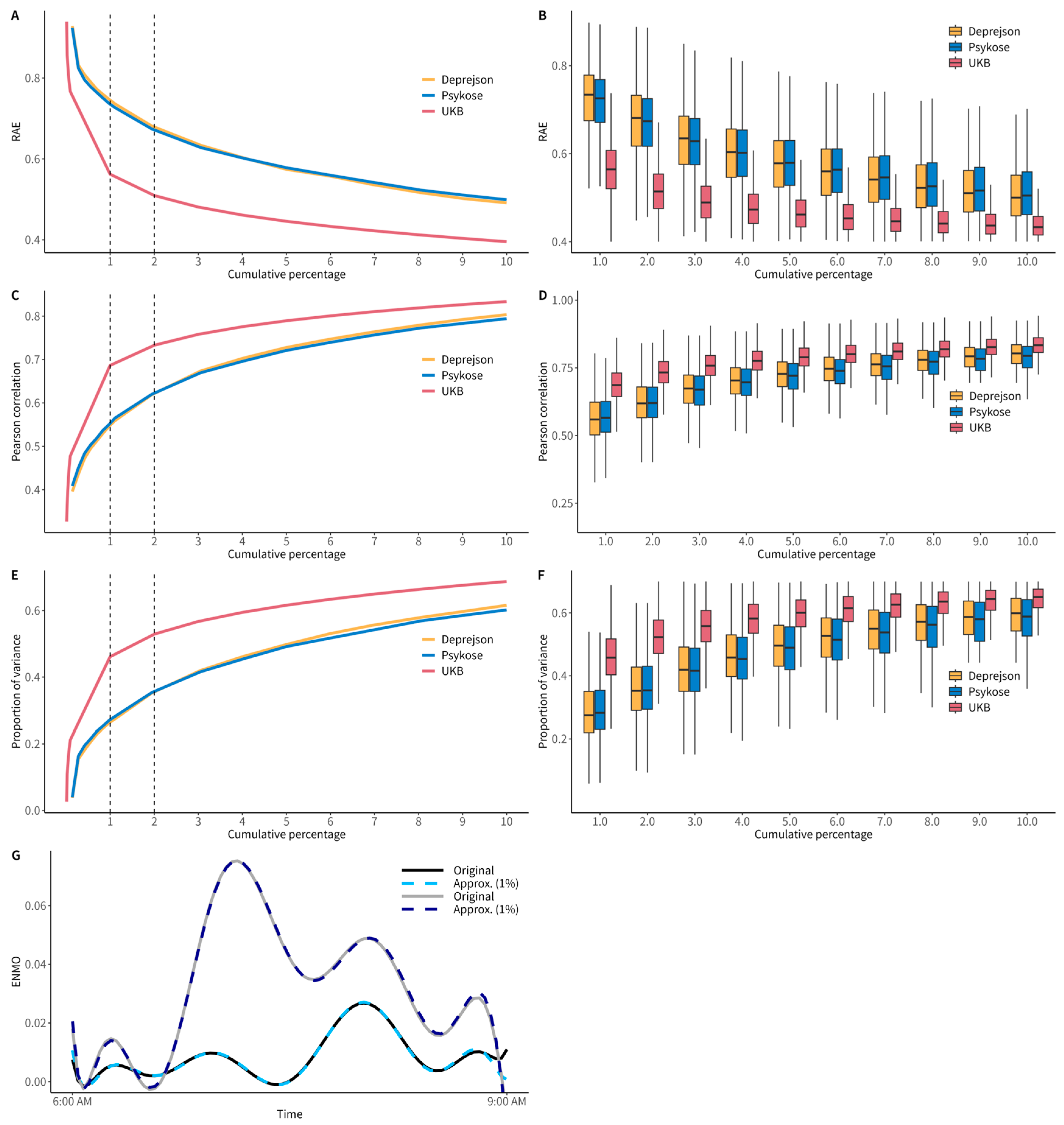
Figure 3 demonstrates the selection of p % DFT variables and the resulting RAE, Pearson correlation, and Expl.var in approximations for three studies. It is essential to note that when utilizing p% DFT features to approximate the original signal, the performance for each individual curve exhibits slight variations. To illustrate this, Figure 3A,C,E present the median results, while Figure 3B,D,F display the results for all individual curves. The overall results show that a small percentage of DFT variables can effectively approximate the original signal, though the exact percentage required varies slightly by dataset. For instance, to achieve a high median Pearson correlation coefficient of approximately 0.8, the UKB dataset required 5.99% of DFT features, while the Psykose and Depresjon datasets required 10% (Figure 3C). Similarly, to achieve a median explained variance (Expl.var) of over 60%, the UKB dataset needed 5% of DFT features, whereas the Psykose and Depresjon datasets again required 10% (Figure 3E). Even a minimal subset, such as 1% waves, consistently achieved an Expl.var ranging from approximately 30% to 55% (Figure 3E,F) and Pearson correlation values above 0.55 (Figure 3C,D) across all three diverse studies. Noting that, despite the variation across individuals (as seen in Figure 3B,D,F), the approximation accurately captures the highs and lows in the curve. The strong performance remains consistent across studies, despite differences in the number of observations per day and the PA metric used in the three studies. Note that in Figure 3, any assigned p percentages come from both the low and high frequency waves. Combinations from both ends encompass both major movement and random noise in PA.

3.2. DFT-Based Variables Are Associated with Group Status and Weekend/Weekday Effects

To explore associations between DFT-derived features and demographic and behavioral factors, we visualized the distributions of log-transformed amplitudes across frequencies (Figure 4). Figure 4A–D illustrate the feature distributions by clinical group (PrBP, PrMDD, and control), weekday/weekend, age group (<60 vs. ≥60 years), and BMI category (underweight, normal, overweight, obesity), respectively. The amplitudes decrease as frequency increases, and the differences among groups become marginal beyond the 20th frequency component; therefore, only the first 20 frequencies are presented. The control group had slightly higher amplitudes across the first 20 frequencies compared to the PrBP and PrMDD groups (Figure 4A). At frequency 1, weekend amplitudes were higher, while at frequency 2, weekday amplitudes were higher; other frequencies showed no significant differences (Figure 4B). Individuals under 60 years old had significantly larger amplitudes (Figure 4C). Individuals with normal weight and those underweight also had significantly larger amplitudes compared to those who were overweight or obese (Figure 4D).
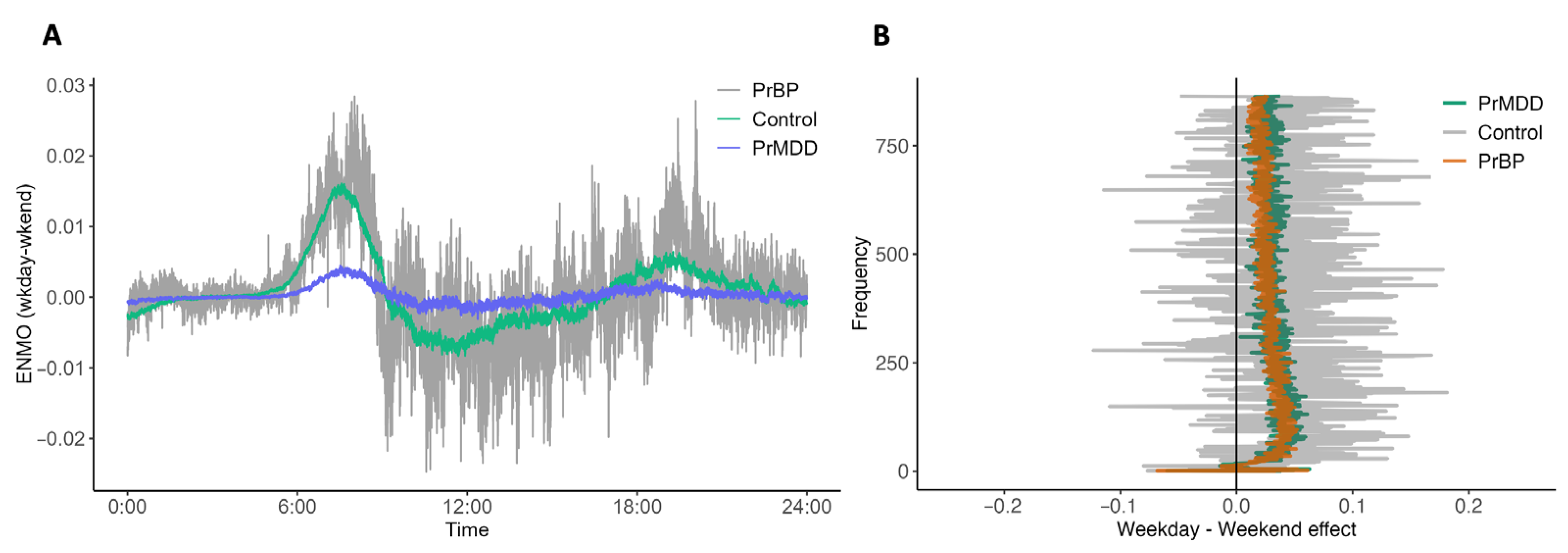
To investigate if the decomposed digital variables are useful in association studies, we examine the relationship between the strength, the amplitude A m j k , and factors such as group status and weekend/weekday effects. We first examine if the three groups, (PrBP, PrMDD, and control) have different activity levels between weekdays and weekends. Figure 5A displays the difference between the average PA on weekdays and on weekends. The degree of difference is group-specific. For instance, the control group has the greatest fluctuation, indicating stronger activity levels during weekdays, especially in early mornings. Participants in the other two groups show similar patterns but with less variability. Particularly, the PrMDD has the least variation.
Next, we adopted a GLMM to accommodate repeated observations (multiple days) per individual at each frequency and to incorporate the interaction between group and weekday effect. For instance, the model in the UKB study is
l o g ( A m j k ) = β 0 k + β 1 k D 1 m + β 2 k D 2 m + β 3 k W m j + β 4 k D 1 m W m j + β 5 k D 2 m W m j + β 6 k Z m + r m k + ε m j k
Note that ( D 1 m , D 2 m ) = (0,0) is for the PrMDD reference group, (1,0) for the PrBP, and (0,1) for the control group. The W m j is 1 if the day is a weekday. Two interaction terms are also added to evaluate if the weekday effect differs across groups. The vectors β 6 k and Z m represent the effects and covariates including age, sex, and BMI. Critically, the term r m k represents the individual-specific random effect, which accounts for the heterogeneity across individuals and the inherent correlation among repeated observations (multiple days) for the same individual. At each frequency ranging from 0 to 864, the weekday-weekend effect is now a combination of coefficient estimates in Equation (3) and is demonstrated in Figure 5B. In the frequency domain, the difference in the control group remains the strongest, even after adjusting for other covariates. The utility of the DFT approach is highlighted by contrasting Figure 5A with Figure 5B. Figure 5A shows that the PrBP group and control group have the most significant fluctuation, indicating a strong weekday-weekend difference, especially in the early mornings. However, Figure 5A also shows that the PrMDD group has the least variability. Figure 5B validates the differentiating power of the DFT features by capturing the group-specific variation in the weekday-weekend effect across all frequencies, relative to the PrMDD reference group. While the time domain analysis emphasizes general fluctuation, the frequency domain analysis successfully translates this complex pattern into quantifiable differences in activity rhythm. The result clearly shows that the control group exhibits the most substantial difference in the low-frequency domain, consistent with higher behavioral flexibility. In contrast, the PrMDD group is confirmed to show the least overall variation. This empirically demonstrates that the DFT features successfully isolate and quantify clinically relevant differences in activity rhythm that are often masked or imprecisely quantified by traditional time-domain analysis.

3.3. Evaluating DFT-Based Variables: Impact on Classification Performance and Variable Influence in Association Studies

This section evaluates the utility of DFT-based variables in two key biomedical studies: classification (prediction) and association (interpretation).
First, we systematically assess whether the inclusion of DFT features improves model performance compared to models using only traditional time-domain summaries for classification. To assess the impact of incorporating DFT variables, we conducted validation using six distinct predictor sets in the classification study: (1) baseline model which only included demographic information such as age and sex; (2) baseline model with rest-activity rhythm (RAR) variables such as L5, M10, relative amplitude (RA = [M10 − L5]/[M10 + L5]) and IV [18]; (3) baseline model with variables form FPCA such as functional principal component (FPC) scores [30]; (4) baseline model with amplitudes from the lowest 1% frequency waves; (5) baseline model with amplitudes from the lowest 1% frequency waves and RAR variable; and (6) baseline model with amplitudes from the lowest 1% frequency waves and FPCA variables. Specifically, FPCA was used to decompose the continuous 24 h activity profiles into FPC scores, and we retained the principal components that cumulatively explained over 80% of the total functional variance for use as predictors.
To ensure both generalizability and interpretability, five machine learning algorithms (Naive Bayes, SVM, logistic regression with lasso, decision tree, and random forest) commonly employed in biomedical and clinical research were selected to provide a comprehensive and balanced evaluation of the DFT-based features. Specifically, the choices encompass a range of model complexities, including linear models, kernel-based separation (SVM), probabilistic approaches (Naive Bayes), and non-linear ensemble/tree-based methods (Decision Tree and Random Forest). This diverse set of classifiers allows us to demonstrate the robustness and general applicability of the DFT-derived variables across different classification paradigms.
The performance was evaluated based on accuracy, sensitivity, specificity, and F1-score from 10 random replications, where each was split into 80% training and 20% testing data, and cross-validation was used to train the model parameters. Note that for the UKB study, only two groups, PrMDD and control, were used in the classification, and the SMOTE algorithm was applied for the imbalance sample.
With the addition of DFT variables, the classification performance improves, as shown in Table 2 for Psykose, Table 3 for the UKB study, and Supplementary Table S4 for Depresjon. The improvement is more substantial than when RAR variables are included, implying the advantage of incorporating DFT variables. The superior informative power of the frequency-domain features is particularly evident when contrasting the feature sets. Among all evaluated models, Random Forest achieved the best overall performance, with a mean accuracy using demographics, RAR, and DFT variables of 0.87 for Psykose, 0.74 for Depresjon, and 0.85 for the UKB study. Note that the improvement is notable in the biobank study: the accuracy with RAR variables under random forest is 0.56 and increases to 0.85 when DFT variables are added to the feature set.
When comparing FPCA variables and DFT variables alone, there is little difference in accuracy and F1 score in the Psykose study. In contrast, the accuracy and F1 score in the Depresjon study and UKB study are slightly better when using only DFT variables. However, if both FPCA variables and DFT variables are used, the model’s performance improves significantly. For example, the Random Forest’s mean accuracy increases from 0.78 when using only FPCA variables to 0.84 in the UKB study after adding DFT variables.
While model performance varied slightly across datasets, this substantial gain—observed consistently across diverse classifiers—underscores that DFT variables improve model accuracy, sensitivity, and specificity. This highlights the robustness and capacity of DFT features to extract highly discriminative information. Furthermore, the results confirm that using both time-domain and DFT features simultaneously achieves the best model performance for large-scale clinical classification tasks.
Beyond classification performance, the utility of DFT-based variables was assessed within the context of biomedical association studies. Prioritizing the field’s requirement for model interpretability to identify and understand risk factors, our analysis focused on the results from interpretable models (i.e., logistic regression and tree-based models). This approach permitted a precise examination of the distinct contributions of both time- and frequency-domain variables to the health outcome.
Model interpretation across the Psykose study (Figure 6), UKB study (Figure 7), and Depresjon study (Supplementary Figure S1) established a crucial role for the DFT features in association studies. In the logistic regression models, RAR variables and demographics generally showed strong positive or negative associations with disease status (odds ratios markedly different from 1). However, DFT features at frequencies 1, 3, and 14 also demonstrated significant associations in the Psykose study (mean OR = 2.085, 1.535, 1.204) (Figure 6A). In contrast, the non-linear algorithms (C5.0 and Random Forest) consistently ranked the DFT features as the most important factors (Figure 6B,C,E,F, and Figure 7B,C,E,F). This pattern was stable across both feature sets and cohorts. This suggests that DFT features may have complex, non-linear relationships with disease status. The high importance of frequency-domain features in tree-based models further reinforces this, strongly indicating that they are essential for capturing these nonlinear relationships. Consequently, incorporating these DFT features is critical in association studies.

3.4. DFT Variables in Simulation Studies for Classification

This simulation study aimed to examine how the DFT features improve the classification performance under different magnitudes of between-individual variation (B.var) and within-individual variation (W.var). Three scenarios were considered, where the ratio of B.var to W.var was set at 1, 2, or 3. Each scenario involved two competing groups, A and B, with 50 individuals in each group. For each individual, five days of PA observations were constructed and the daily PA was composed of observations generated based on 1440 frequency waves and random variation. Details of the settings are listed in Appendix A.3.
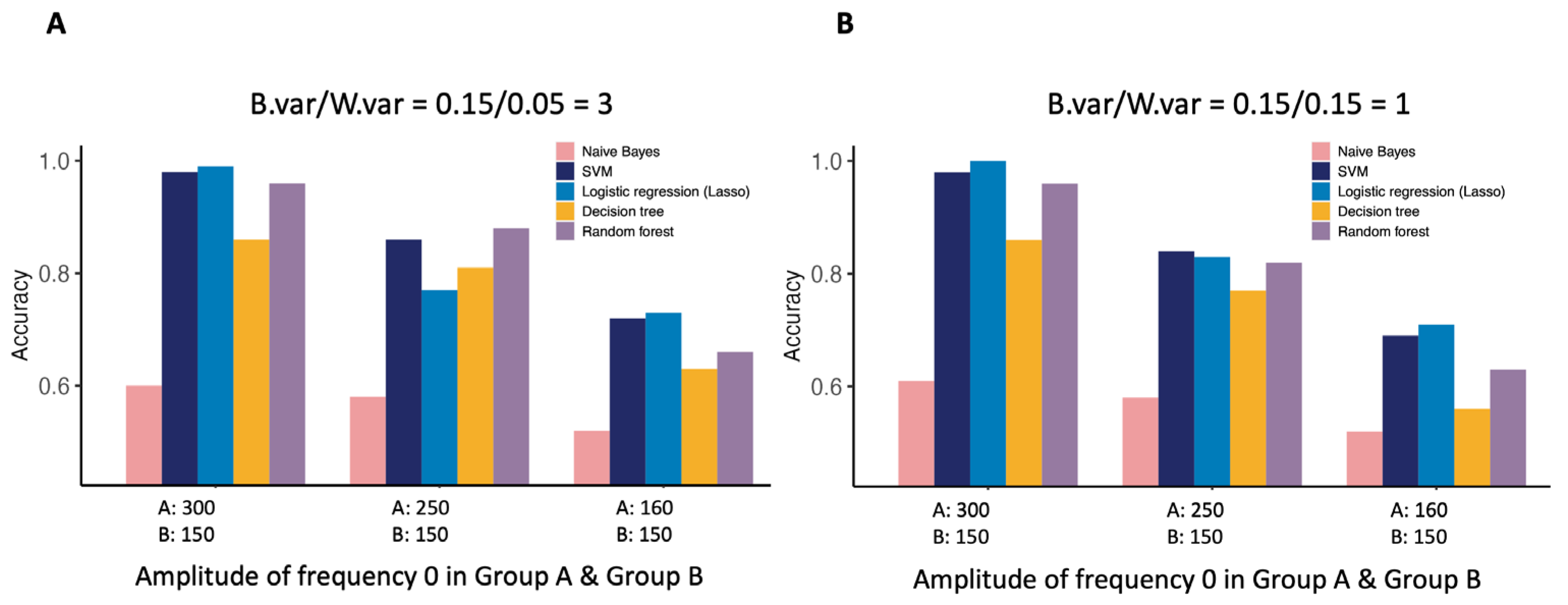
Based on the estimated amplitudes of frequencies 0–4, the classification performance under two scenarios, along with the corresponding amplitudes of frequency 0, is summarized in Figure 8.
The study’s primary objective was to validate the robustness of the DFT features against varying levels of heterogeneity, which is a critical challenge in real-world wearable PA data. As shown in Figure 8, most of the classifiers, except Naïve Bayes, provide high accuracy. The accuracy values remain robustly high, ranging between 1.0 and 0.8, even as the difference in the core DFT feature (amplitude of frequency 0) between the two groups decreases significantly (from 300 vs. 150 to 160 vs. 150). This pattern persists when the ratio of between-individual variation to within-individual variation, B.var/W.var, is 3 or 1, as shown in Figure 8A,B. This empirical confirmation shows that the DFT-derived features retain their stability and predictive power even when complex intra-and inter-individual variation is present, making them reliable for real-world group distinction. Results under other scenarios are similar and detailed in Supplementary Figure S2.

4. Discussion

Previous research often averages PA data per second or minute and calculates summary statistics to reduce overall data volume and minimize correlations across days. Such procedures are easy and efficient, but may overlook the nature of temporal relationships and informative variation in the data. The DFT presents a favorable alternative for its ability to represent the temporal pattern, where the information associated with time trends can be stored in the periodic waves. While the DFT produces waves of the same number as that of the observation time points, the dimension reduction becomes easier and more intuitive with these DFT variables. Applications in the three motivating studies showed that, with even 1% of the waves, the approximation can achieve high accuracy.
This research demonstrates the advantages of utilizing frequency-domain digital variables in analysis of physical activity. The DFT approach offers a decomposition of the original time series, expressing temporal trends through a set of waves that capture the same information as the original PA in the time domain. This decomposition leads to a novel and efficient way of dimension reduction, where such reduction is less straightforward in the original time domain. The reduced set of DFT-based PA retains most information contained in the original PA. The derived DFT features can be applied in statistical and machine learning models, resulting in a large improvement in classification accuracy. With the increasing prevalence of digital data collection and utilization, the development of a new analysis methodology is essential. Application of these analyses may be implemented to identify individuals who need special care or to detect early changes in behaviors.
When the DFT variables were applied in the evaluation of the weekday/weekend effect for various response groups in the UKB study, both the control and PrMDD groups exhibited a significant difference in activity between different days. In addition, these digital phenotypes have demonstrated dependence not only on time-dependent variables but also on time-independent factors, such as age, sex, BMI status, and probable mental status. This association between physical activity and these factors has been previously noted [31,32], providing support for employing the DFT variable as proxies of the original temporal PA observations in future research including association analysis and machine learning classification and prediction.
This study has limitations. First, we select DFT-features based on frequency to reflect the focus on approximating free-living PA’s. If the research goal is to capture unique movements during a predetermined time interval, then a selection based on magnitudes of amplitude may be preferred. That is, the selection procedure should be objective dependent. If the aim is to capture large and abrupt movements, then the amplitude-based approximation may provide better and faster approximations. The second limitation is the applicability of the DFT-based PA features. As demonstrated here, it is only feasible to conduct internal validations. This is because the study population and heterogeneity pattern may be incompatible between studies. In other words, the classification features derived from one study may not be appropriate for another study. Therefore, it is advised to recruit large samples, including a large number of individuals and of days, so that further validation can be carried out. Third, the low-frequency DFT variables for classification in three application studies may not adequately represent the small or specific movements occurring in shorter time periods or be suitable for differentiating certain types of activities. For instance, the conclusions of a few DFT-based variables may not be applicable when detecting or classifying movements such as sleep/wake detection or classification of manual movements. Further studies would be necessary to investigate the utility of high-frequency DFT variables in this context and to compare with existing methods, such as the hidden Markov Model or Wavelet analysis, designed for monitoring circadian rhythms [33,34].

Supplementary Materials

The following supporting information can be downloaded at https://www.mdpi.com/article/10.3390/math13223616/s1, Figure S1: Comparative feature contributions to classification models for Depresjon study, Figure S2: Accuracy of five classification tools in simulation studies; Table S1: Summary of demographic information in the UK Biobank study; Table S2: Summary of demographic information in the Depresjon study; Table S3: Summary of demographic information in the Psykose study; Table S4: Values (average and standard error in parentheses) of the evaluation criteria (Accuracy, Sensitivity, Specificity, and F1-score) under various classification tools for the Depresjon study.

Author Contributions

Y.-T.L.: Writing—original draft, Writing—review and editing, Methodology, Data analysis, Conceptualization, Visualization. C.K.H.: Writing—original draft, Writing—review and editing, Investigation, Methodology, Data analysis, Data curation, Conceptualization, Funding acquisition, Visualization. A.C.: Writing—review and editing, Investigation, Resources. T.-P.L.: Writing—review and editing, Investigation, Resources. P.-H.K.: Writing—review and editing, Investigation, Resources. C.W.: Writing—original draft, Writing—review and editing, Supervision, Methodology, Conceptualization, Funding acquisition. All authors have read and agreed to the published version of the manuscript.

Funding

This study was supported in part by the Ministry of Science and Technology (grant number MOST-110-2314-B-002-078-MY3; NSTC-113-2314-B-002-177-MY3; NSTC-113-2314-B-002-176) and National Taiwan University Higher Education Sprout Project (grant number NTU-111L881002).

Data Availability Statement

The datasets supporting the conclusions of this article are available in (1) the UK Biobank data portal with applications through https://www.ukbiobank.ac.uk/ (accessed on 20 March 2024), (2) the Depresjon study http://datasets.simula.no/depresjon/ (accessed on 1 June 2025), and (3) the Psykose study https://datasets.simula.no/psykose/ (accessed on 1 June 2025).

Acknowledgments

This research has been conducted using the UK Biobank Resource under Application Number 134902. During the preparation of this manuscript, the authors used ChatGPT (GPT-5), Google Gemini 2.5 and Grammarly 1.141.2.0 for the purposes of English editing and grammar checking. The authors have reviewed and edited the output and take full responsibility for the content of this publication.

Conflicts of Interest

The authors declare no conflicts of interest.

Abbreviations

The following abbreviations are used in this manuscript:
ACActivity count
AIActivity index
BMIBody Mass Index
ENMOEuclidean Norm Minus One
FFTFast Fourier transform
FPCFunctional Principal Component
FPCAFunctional Principal Component Analysis
GLMMGeneralized linear mixed-effect model
IFFTInverse fast Fourier transform
ISInter-day stability
IVIntra-day variability
L5The least active 5 h
M10The most active 10 h
PAPhysical activity
PrBPProbable bipolar
PrMDDProbable major depression
RARelative amplitude
RAERelative absolute error
RARRest-activity rhythm
SMOTESynthesized minority oversampling technique
SPTThe sleep period time
SVMSupport vector machine
UKBUK Biobank

Appendix A

Appendix A.1. Three Motivating Studies

The UK Biobank study recruited more than half a million volunteer participants. Among them, a total of 103,688 individuals consented to wear a wrist-worn accelerometer, specifically the Axivity Ax3, which sampled at 100 Hz for a duration of 7 days to monitor their daily activity. The acceleration metric considered for analysis was the Euclidean Norm Minus One (ENMO), which combines the triaxial accelerations ( a c c x , a c c y , a c c z , ) with the equation:
E N M O = m a x a c c x 2 + a c c y 2 + a c c z 2 1,0
The value of ENMO ranged from 0 to 8 g, and the number of recorded activity level per day was 17,280. Data management procedures involved automatic calibration, non-wear time detection, a five-second median filter, and calculation of acceleration metric. The GGIR package (ver.2.3.0) in R was employed for quality control and processing [35], following the same procedures used in Su [36] for data screening. Ethical approval for the UK Biobank study was granted by the National Information Governance Board for Health and Social care and the NHS North West Multicentre Research Ethics Service (11/NW/0382). Written informed consent was obtained from all study participants by UKB research group. The data can be accessed with application through https://www.ukbiobank.ac.uk/ (accessed on 20 March 2024). The probable history of mental health status, probable bipolar or probable major depression, was adopted as the outcome variable [37]. The resulting individuals included 15,252 control (CN) participants, 158 probable bipolar disorder (PrBP) individuals, and 5667 probable major depressive depression (PrMDD) individuals, bringing the total number of individuals to 21,077.
The second study, Depresjon [27], recruited individuals whose mental health status was determined based on the Montgomery-Asberg Depression Rating Scale (MADRS). Among the participants, 23 scored higher than 30 on the MADRES and were defined as having severe depression, while 32 were categorized as not having depressive symptoms and formed the control group. Their Activity counts, scaled by accelerations per minute, were generated from the raw acceleration data recorded by Actiwatch at 32 Hz. Among the 23 patients with severe depression, data from 5 were collected during their hospitalization, while the data from the remaining 18 patients were recorded during outpatient visits. A total of 739 days were retained for analysis, of which 306 days were from unipolar and bipolar depressed patients and 433 days were from individuals in the control group, averaging 13–14 days per person. Each day consisted of 1440 activity counts, where each count was a one-minute total activity count ranging between 0 and 3000. To maintain manageable amplitude values, the collected activity counts were divided by 1000 before FFT. The additional baseline information can be found in Supplementary Table S2. Data quality control and management procedures to retain days for further analysis are described in Supplementary Figure S2 in the Supporting Information. The collected data of Depresjon study are available for download from http://datasets.simula.no/depresjon/ (accessed on 1 June 2025). Ethical approval for this study was granted by the Norwegian Regional Medical Research Ethics Committee West (REK III, Health-West, Norway) [38] and written informed consent was obtained from every participant [39].
The third mental health study, Psykose [28], focused on 22 schizophrenia patients hospitalized at a psychiatric ward at Haukeland University Hospital. This study shared the same 32 control individuals in the Depresjon study. The same accelerometer, Actiwatch at 32 Hz, was used and the procedures of data management were the same as that for Depresjon (details in Supplementary Figure S2). After data management including quality control, the number of retained days for analysis was 729, of which 296 days were from schizophrenia patients and 433 days from control individuals, averaging 13–14 days per individual. Supplementary Table S3 displays the demographic information for the Psykose study. The data of Psykose study can be downloaded from https://datasets.simula.no/psykose/ (accessed on 1 June 2025). The ethical approval for the study was granted by the Norwegian Regional Medical Research Ethics Committee West [38].

Appendix A.2. Definition of RAE and Expl.var

The relative absolute error (RAE) is defined as the following summation over all individuals (indexed by m ) and across all days (indexed by j ),
R A E m , j = t = 0 T 1 | x ^ m j t x m j ( t ) | t = 0 T 1 | x m j ( t ) x ¯ m j | .
The x ¯ m j in the denominator is the average of x m j ( t ) over t . A lower RAE implies better approximations. The Y axis in Figure 3A indicates the median across all possible ( i , j ).
The proportion of explained variance measures the proportion of variance explained by the approximated physical activity levels among the variance of the original observations for each PA curve:
E x p l . v a r m , j = V a r ( { x ^ m j ( t ) :   t } ) / V a r ( { x m j ( t ) :   t } )
A larger Expl.var implies that the approximated curves provide closer variability of the original curves. The Y axis in Figure 3C indicates the median across all possible ( m , j ).

Appendix A.3. Simulation Settings

Individuals in two groups (A and B) are to be classified based on 5 days of PA observations per person. The daily PA was constructed based on 1440 frequency waves, denoted as R ( k ) + I ( k ) i with frequency k = 0 , 1 , , 1439 . These frequency waves highlight the difference between groups A and B. The value of ( R ( k ) , I ( k ) ) when k = 0 was set at (300,0), (250,0), or (160,0) in group A and at a constant (150,0) in group B. When k = 1 ~ 72 , the values of ( R ( k ) , I ( k ) ) in group A was chosen similar to the average value of those in the Psykose study; while the corresponding value in group B was ( R ( k ) a k , I k b ( k ) ) or ( R ( k ) a k / 2 , I k b k / 2 ) , indicating a difference of ( a ( k ) , b ( k ) ) or ( a k / 2 , b k / 2 ) from the values in group A.
Once the group-specific average PA curve was determined, individual daily curves were then formulated by adding an individual-specific random variation from N ( 0 , σ B 2 ) and a time-specific variation from N ( 0 , σ W 2 ) . The σ B 2 represents the between-individual variation and was set at 0.15, while the within-individual variation σ W 2 was set at 0.05, 0.10, or 0.15, respectively. Note that the above two types of variation only occurred between 5 in the morning and 9:30 at night, while the variance was set at 0.01 for the rest of the day to indicate similar behavior during the time in sleep or rest. In other words, the σ B 2 and σ W 2 are not statistically defined between- and within-individual variance but are convenient definitions in this simulation study. After constructing the daily PA curve, the procedure to retrieve the DFT digital variables was implemented, and the amplitudes of the first five lowest frequencies were used to classify the 100 individuals using the algorithms considered in the previous section.

Appendix B. Mathematical Framework: Sparse Fourier Approximation Proof

This section presents the mathematical foundation for our claim: a small fraction of FFT coefficients suffices to approximate smooth time series signals accurately. The result supports our empirical observation that preserving only ~1% of the spectrum yields negligible reconstruction error.

Appendix B.1. Preliminaries

Let f   C r π ,   π   L 2 ( [ π ,   π ] ) be a real-valued, 2 π -periodic function with r -times continuously differentiable derivatives.
  • Fourier Basis Theorem: the set  1 2 , cos n x , sin n x n = 1 ,   2 ,   }  forms an orthogonal basis for  L 2 π ,   π .  Then, any  f  admits the expansion 
    f x = a 0 2 + n = 1 [ a n cos n x + b n s i n ( n x ) ] ,
    where a 0 = 1 π   π π f x d x , a n = 1 π π π f ( x ) c o s ( n x ) d x , b n = 1 π π π f ( x ) s i n ( n x ) d x
  • Parseval’s Identity
    f L 2 2 = 1 π π π f x 2 d x = a 0 2 2 + n = 1 ( a n 2 + b n 2 )
    which states that the total time-domain energy equals the sum of squared Fourier coefficients.

Appendix B.2. Coefficient Decay for Smooth Signals

  • Lemma (Coefficient Bound).
  • If f C r π ,   π , then a n ,   b n C n r + 1 , C = 1 π f r + 1 L 1
Smoothness (larger r ) causes faster spectral decay, which justifies aggressive frequency-domain truncation. In practice, this can be empirically checked by plotting log a n v s .   l o g n and inspecting the slope.
  • Main Theorem.
  • Let f   C r π ,   π , and N be the total number of FFT modes. Let δ be the proportion of the selected FFT modes and M = δ N . Define the truncated sum keeping only M modes from both ends:
    f ~ ( x ) = a 0 2 + n = 1 M a n cos n x + b n s i n ( n x ) + n = N M + 1 N a n cos n x + b n s i n ( n x )
    Then, f x f ~ x L 2 C M r , C = 1 r C .
Proof 
 
(1)
Parseval’s Identity:
f x f ~ x L 2 2 = n I ( a n 2 + b n 2 ) ,   w h e r e   I = 1 , , M { N M + 1 , , N }
(2)
Apply coefficient bound:
n > M ( a n 2 + b n 2 ) 2 C 2 n = M + 1 1 n 2 ( r + 1 )
(3)
Estimate Tail Sum:
n > M 1 n 2 ( r + 1 ) 1 2 r M 2 r
(4)
Square Root:
f x f ~ x L 2   1 r C M r
  • Remark
By Sharper Sparsity, choosing δ = 0.005 (0.5% from each end) still yields
f x f ~ x L 2 C 0.005 N r , w h e r e   C = 1 r C
indicating that the approximation error decays rapidly for smooth signals. This result further supports our empirical finding that preserving only 1% of FFT coefficients is sufficient to accurately approximate smooth physiological time series, such as PA curves.

References

  1. Straczkiewicz, M.; James, P.; Onnela, J.P. A systematic review of smartphone-based human activity recognition methods for health research. npj Digit. Med. 2021, 4, 148. [Google Scholar] [CrossRef] [PubMed]
  2. Babu, M.; Lautman, Z.; Lin, X.; Sobota, M.; Snyder, M. Wearable devices: Implications for precision medicine and the future of health care. Annu. Rev. Med. 2024, 75, 401–415. [Google Scholar] [CrossRef]
  3. Lee, T.; Chen, C.; Chen, I.; Chen, H.; Liu, C.; Wu, S.; Hsiao, C.K.; Kuo, P.-H. Dynamic bidirectional associations between global positioning system mobility and ecological momentary assessment of mood symptoms in mood disorders: Prospective cohort study. J. Med. Internet Res. 2024, 26, e55635. [Google Scholar] [CrossRef]
  4. Opoku Asare, K.; Terhorst, Y.; Vega, J.; Peltonen, E.; Lagerspetz, E.; Ferreira, D. Predicting depression from smartphone behavioral markers using machine learning methods, hyperparameter optimization, and feature importance analysis: Exploratory study. JMIR Mhealth Uhealth 2021, 9, e26540. [Google Scholar] [CrossRef]
  5. Jeganathan, V.S.; Golbus, J.R.; Gupta, K.; Luff, E.; Dempsey, W.; Boyden, T.; Rubenfire, M.; Mukherjee, B.; Klasnja, P.; Kheterpal, S.; et al. Virtual AppLication-supported Environment To INcrease Exercise (VALENTINE) during cardiac rehabilitation study: Rationale and design. Am. Heart J. 2022, 248, 53–62. [Google Scholar] [CrossRef]
  6. Leroux, A.; Xu, S.; Kundu, P.; Muschelli, J.; Smirnova, E.; Chatterjee, N.; Crainiceanu, C. Quantifying the predictive performance of objectively measured physical activity on mortality in the UK Biobank. J. Gerontol. A Biol. Sci. Med. Sci. 2021, 76, 1486–1494. [Google Scholar] [CrossRef]
  7. Graham, B.; Farrell, M. Mortality prediction using data from wearable activity trackers and individual characteristics: An explainable artificial intelligence approach. Expert. Syst. Appl. 2025, 267, 126195. [Google Scholar] [CrossRef]
  8. Boruvka, A.; Almirall, D.; Witkiewitz, K.; Murphy, S.K. Assessing time-varying causal effect moderation in mobile health. J. Am. Stat. Assoc. 2018, 113, 1112–1121. [Google Scholar] [CrossRef] [PubMed]
  9. NeCamp, T.; Sen, S.; Frank, E.; Walton, M.A.; Ionides, E.L.; Fang, Y.; Tewari, A.; Wu, Z. Assessing real-time moderation for developing adaptive mobile health interventions for medical interns: Micro-randomized trial. J. Med. Internet Res. 2020, 22, e15033. [Google Scholar] [CrossRef]
  10. Golbus, J.R.; Dempsey, W.; Jackson, E.A.; Nallamothu, B.K.; Klasnja, P. Microrandomized trial design for evaluating just-in-time adaptive interventions through mobile health technologies for cardiovascular disease. Circ. Cardiovasc. Qual. Outcomes 2021, 14, e006760. [Google Scholar] [CrossRef] [PubMed]
  11. Doherty, A.; Jackson, D.; Hammerla, N.; Plötz, T.; Olivier, P.; Granat, M.H.; White, T.; van Hees, V.T.; Trenell, M.I.; Owen, C.G.; et al. Large scale population assessment of physical activity using wrist worn accelerometers: The UK biobank study. PLoS ONE 2017, 12, e0169649. [Google Scholar] [CrossRef]
  12. Bai, J.; Di, C.; Xiao, L.; Evenson, K.R.; LaCroix, A.Z.; Crainiceanu, C.M.; Buchner, D.M. An activity index for raw accelerometry data and its comparison with other activity metrics. PLoS ONE 2016, 11, e0160644. [Google Scholar] [CrossRef]
  13. van Hees, V.T.; Gorzelniak, L.; Dean León, E.C.; Eder, M.; Pias, M.; Taherian, S.; Ekelund, U.; Renström, F.; Franks, P.W.; Horsch, A.; et al. Separating movement and gravity components in an acceleration signal and implications for the assessment of human daily physical activity. PLoS ONE 2013, 8, e61691. [Google Scholar] [CrossRef]
  14. van Hees, V.T.; Sabia, S.; Jones, S.E.; Wood, A.R.; Anderson, K.N.; Kivimäki, M.; Frayling, T.M.; Pack, A.I.; Bucan, M.; Trenell, M.I.; et al. Estimating sleep parameters using an accelerometer without sleep diary. Sci. Rep. 2018, 8, 12975. [Google Scholar] [CrossRef] [PubMed]
  15. van Hees, V.T.; Migueles, J.; Fang, Z.; Zhao, J.; Heywood, J.; Mirkes, E.; Sabia, S.; Patterson, M.R.; Pujol, J.C.; Kushleyeva, L.; et al. R Package GGIR: Raw Accelerometer Data Analysis. Version 2.3.0. Available online: https://CRAN.R-project.org/package=GGIR (accessed on 7 June 2023).
  16. Bai, J.; Goldsmith, J.; Caffo, B.; Glass, T.A.; Crainiceanu, C.M. Movelets: A dictionary of movement. Electron. J. Stat. 2012, 6, 559–578. [Google Scholar] [CrossRef] [PubMed]
  17. Xue, X.N.; Qi, Q.; Sotres-Alvarez, D.; Roesch, S.C.; Llabre, M.M.; Bainter, S.A.; Mossavar-Rahmani, Y.; Kaplan, R.; Wang, T. Modeling daily and weekly moderate and vigorous physical activity using zero-inflated mixture Poisson distribution. Stat. Med. 2020, 39, 4687–4703. [Google Scholar] [CrossRef]
  18. Van Someren, E.J.; Swaab, D.F.; Colenda, C.C.; Cohen, W.; McCall, W.V.; Rosenquist, P.B. Bright light therapy: Improved sensitivity to its effects on rest-activity rhythms in Alzheimer patients by application of nonparametric methods. Chronobiol. Int. 1999, 16, 505–518. [Google Scholar] [CrossRef]
  19. Feng, H.; Yang, L.; Ai, S.; Liu, Y.; Zhang, W.; Lei, B.; Chen, J.; Liu, Y.; Chan, J.W.Y.; Chan, N.Y.; et al. Association between accelerometer-measured amplitude of rest-activity rhythm and future health risk: A prospective cohort study of the UK Biobank. Lancet Healthy Longev. 2023, 4, e200–e210. [Google Scholar] [CrossRef]
  20. Rykov, Y.; Thach, T.Q.; Bojic, I.; Christopoulos, G.; Car, J. Digital biomarkers for depression screening with wearable devices: Cross-sectional study with machine learning modeling. JMIR Mhealth Uhealth 2021, 9, e24872. [Google Scholar] [CrossRef] [PubMed]
  21. Zhang, Y.; Li, H.; Keadle, S.K.; Matthews, C.E.; Carroll, R.J. A review of statistical analyses on physical activity data collected from accelerometers. Stat. Biosci. 2019, 11, 465–476. [Google Scholar] [CrossRef]
  22. Ashraf, M.; Anowar, F.; Setu, J.H.; Chowdhury, A.I.; Ahmed, E.; Islam, A.; Al-Mamun, A. A survey on dimensionality reduction techniques for time-series data. IEEE Access 2023, 11, 42909–42923. [Google Scholar] [CrossRef]
  23. Sharma, A.; Purwar, A.; Lee, Y.D.; Lee, Y.S.; Chung, W.Y. Frequency based classification of activities using accelerometer data. In Proceedings of the 2008 IEEE International Conference on Multisensor Fusion and Integration for Intelligent Systems, Seoul, Republic of Korea, 20–22 August 2008; IEEE: New York, NY, USA, 2008. [Google Scholar]
  24. Cochran, W.T.; Cooley, J.W.; Favin, D.L.; Helms, H.D.; Kaenel, R.A.; Lang, W.W.; Maling, G.C.; Nelson, D.E.; Rader, C.M.; Welch, P.D. What is the fast Fourier transform? Proc. IEEE 1967, 55, 1664–1674. [Google Scholar] [CrossRef]
  25. Vähä-Ypyä, H.; Vasankari, T.; Husu, P.; Suni, J.; Sievänen, H. A universal, accurate intensity-based classification of different physical activities using raw data of accelerometer. Clin. Physiol. Funct. Imaging 2015, 35, 64–70. [Google Scholar] [CrossRef] [PubMed]
  26. Belcher, B.R.; Berrigan, D.; Dodd, K.W.; Emken, B.A.; Chou, C.P.; Spruijt-Metz, D. Physical activity in US youth: Impact of race/ethnicity, age, gender, & weight status. Med. Sci. Sports Exerc. 2010, 42, 2211–2221. [Google Scholar] [CrossRef]
  27. Garcia-Ceja, E.; Riegler, M.; Jakobsen, P.; Tørresen, J.; Nordgreen, T.; Oedegaard, K.J.; Fasmer, O.B. Depresjon: A motor activity database of depression episodes in unipolar and bipolar patients. In Proceedings of the 9th ACM Multimedia Systems Conference, Amsterdam, The Netherlands, 12–15 June 2018. [Google Scholar]
  28. Jakobsen, P.; Garcia-Ceja, E.; Stabell, L.A.; Oedegaard, K.J.; Berle, J.O.; Thambawita, V.; Hicks, S.A.; Halvorsen, P.; Fasmer, O.B.; Riegler, M.A. Psykose: A motor activity database of patients with schizophrenia. In Proceedings of the 2020 IEEE 33rd International Symposium on Computer-Based Medical Systems, Rochester, MN, USA, 28–30 July 2020. [Google Scholar]
  29. Bhatia, R. Convergence in L2 and L1. In Fourier Series; American Mathematical Society/MAA Press: Washington, DC, USA, 2005; Chapter 4. [Google Scholar] [CrossRef]
  30. Ramsay, J.O.; Silverman, B.W. Functional Data Analysis; Springer: New York, NY, USA, 2005. [Google Scholar]
  31. Black, M.; Brunet, J. Exploring the effect of an eHealth intervention on women’s physical activity: Design and rationale for a randomized controlled trial. Digit. Health 2022, 8, 20552076221093134. [Google Scholar] [CrossRef]
  32. Ramirez, V.; Shokri-Kojori, E.; Cabrera, E.A.; Wiers, C.E.; Merikangas, K.; Tomasi, D.; Wang, G.-J.; Volkow, N.D. Physical activity measured with wrist and ankle accelerometers: Age, gender, and BMI effects. PLoS ONE 2018, 13, e0195996. [Google Scholar] [CrossRef]
  33. Li, X.; Zhang, Y.; Jiang, F.; Zhao, H. A novel machine learning unsupervised algorithm for sleep/wake identification using actigraphy. Chronobiol. Int. 2020, 37, 1002–1015. [Google Scholar] [CrossRef] [PubMed]
  34. Ogbagaber, S.B.; Cui, Y.; Li, K.; Iannotti, R.J.; Albert, P.S. A hidden Markov modeling approach combining objective measure of activity and subjective measure of self-reported sleep to estimate the sleep-wake cycle. J. Appl. Stat. 2022, 51, 370–387. [Google Scholar] [CrossRef]
  35. Migueles, J.H.; Rowlands, A.V.; Huber, F.; Sabia, S.; van Hees, V.T. GGIR: A research community–driven open source R package for generating physical activity and sleep outcomes from multi-day raw accelerometer data. J. Meas. Phys. Behav. 2019, 2, 188–196. [Google Scholar] [CrossRef]
  36. Su, C.H. An Exploratory Analysis of Sleep and Activity Variables from Wearable Device in UK Biobank Study. Master’s thesis, National Taiwan University, Taipei, Taiwan, 2022.
  37. Smith, D.J.; Nicholl, B.I.; Cullen, B.; Martin, D.; Ul-Haq, Z.; Evans, J.; Gill, J.M.R.; Roberts, B.; Gallacher, J.; Mackay, D.; et al. Prevalence and characteristics of probable major depression and bipolar disorder within UK biobank: Cross-sectional study of 172,751 participants. PLoS ONE 2013, 8, e75362. [Google Scholar] [CrossRef] [PubMed]
  38. Berle, J.O.; Hauge, E.R.; Oedegaard, K.J.; Holsten, F.; Fasmer, O.B. Actigraphic registration of motor activity reveals a more structured behavioural pattern in schizophrenia than in major depression. BMC Res. Notes 2010, 3, 149. [Google Scholar] [CrossRef] [PubMed]
  39. Jakobsen, P.; Garcia-Ceja, E.; Riegler, M.; Stabell, L.A.; Nordgreen, T.; Torresen, J.; Fasmer, O.B.; Oedegaard, K.J. Applying machine learning in motor activity time series of depressed bipolar and unipolar patients compared to healthy controls. PLoS ONE 2020, 15, e0231995. [Google Scholar] [CrossRef] [PubMed]
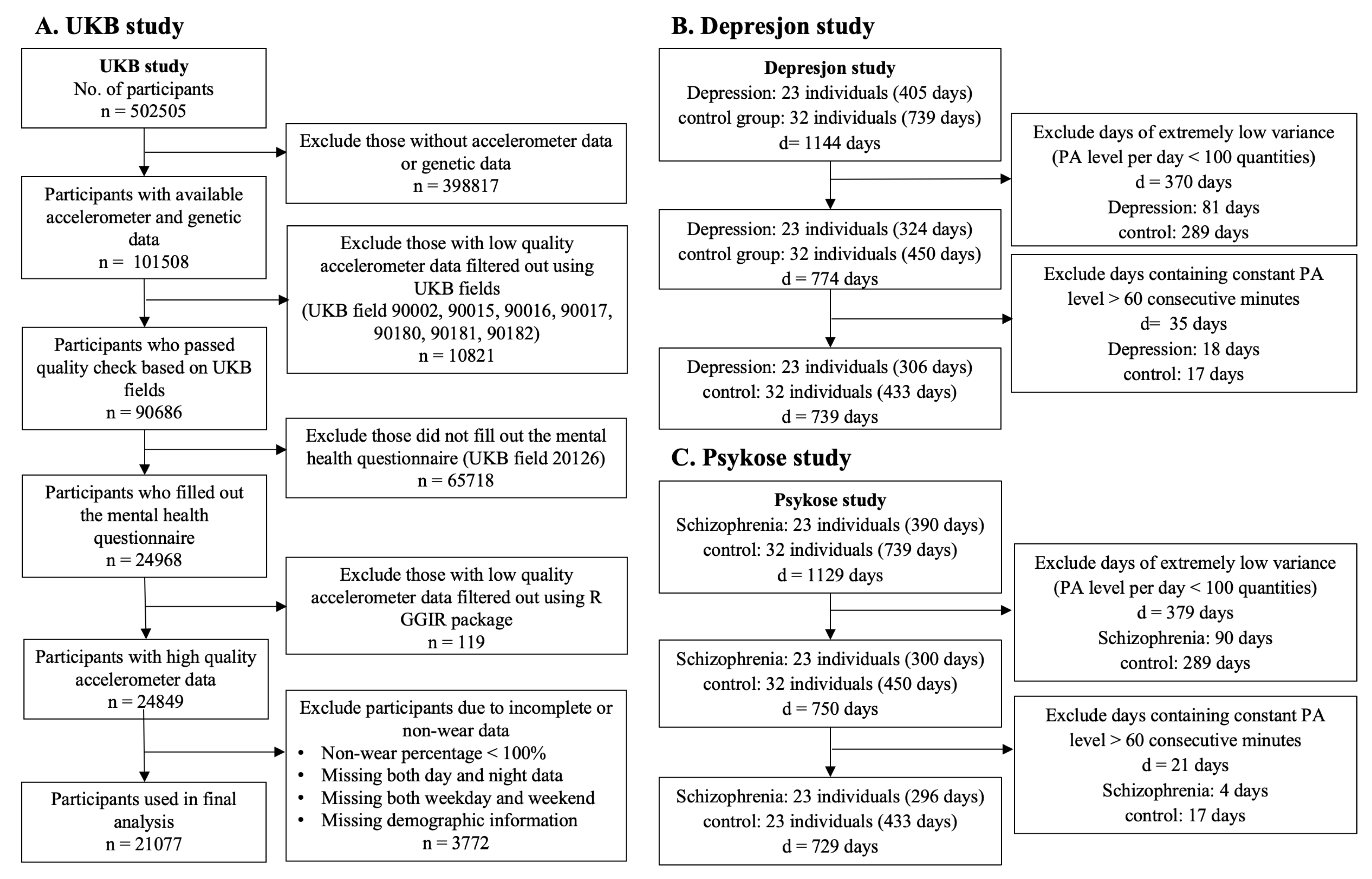
Figure 1. Flowcharts of the digital data management in the three studies. (A) UK Biobank. (B) Depresjon. (C) Psykose.
Mathematics 13 03616 g001
Figure 2. Illustrations of transformations and approximation procedures.
Mathematics 13 03616 g002
Figure 3. Approximation evaluation with different proportions of DFT waves in three studies. (A) Median RAE across all individuals. (B) Distribution of individual RAE values. (C) Median Pearson correlation across all individuals. (D) Distribution of individual Pearson correlation. (E) Median proportion of explained variance across all individuals. (F) Distribution of individual proportion of explained variance. (G) The original and approximated PA for two randomly selected individuals.
Mathematics 13 03616 g003
Figure 4. Distributions of DFT-derived feature amplitudes across different factors. (A) clinical groups: PrBP, PrMDD, and control. (B) Weekday versus weekend. (C) Age groups (<60 vs. ≥60 years). (D) BMI categories (underweight, normal, overweight, obesity).
Mathematics 13 03616 g004
Figure 5. Difference in activity levels between weekdays and weekends. (A) Difference between the average ENMO among weekdays and that among weekends for each group. (B) The weekday and weekend difference is displayed at each frequency. Differences were estimated using a generalized linear mixed-effect model.
Mathematics 13 03616 g005
Figure 6. Comparative feature contributions to association models for the Psykose study. The figure compares feature contributions across three models using two feature sets from 10 random replications. The Top Row (AC) presents results for the RAR variables + DFT feature set, and the Bottom Row (DF) presents results for the FPCA + DFT feature set. (A,D) show the odds ratio from the LASSO logistic regression model. (B,E) show importance values from the C5.0 model. (C,F) show importance values from the random forest model.
Mathematics 13 03616 g006
Figure 7. Comparative feature contributions to association models for the UKB study. The figure compares feature contributions across three models using two feature sets from 10 random replications. Only the top 25 features ranked by importance or effect size are displayed. The top row (AC) presents results for the RAR variables + DFT feature set, and the bottom row (DF) presents results for the FPCA + DFT feature set. (A,D) show the odds ratio from the LASSO logistic regression model. (B,E) show importance values from the C5.0 model. (C,F) show importance values from the random forest model.
Mathematics 13 03616 g007
Figure 8. Simulation studies of classification accuracy of five machine learning tools under different settings of between- and within-individual variance. (A) illustrates the classification accuracy results when the ratio of between-individual variance (B.var) to within-individual variance (W.var) is 3, while (B) presents the results for the ratio of 1.
Mathematics 13 03616 g008
Table 1. Descriptions of data for the final analysis of each motivating study.
UK BiobankPsykoseDepresjon
Sample size21,0775455
Age range40~7021~6921~69
Sex F:M11,500:957723:3130:25
Wearable deviceAxivity Ax3Actiwatch AW4Actiwatch AW4
Sampling frequency100 Hz32 Hz32 Hz
Metric of PA levelENMOActivity countActivity count
Range of PA level0~8 g0~80~8
No. of observations per day for analysis17,28014401440
No. of available days per individual2~66~219~21
Table 2. Values (average and standard error in parentheses) of the evaluation criteria (Accuracy, Sensitivity, Specificity, and F1-score) under various classification tools for the Psykose study.
AccuracySensitivitySpecificityF1 Score
Baseline model (demographic information)
Naive Bayes0.72 (0.013)0.61 (0.035)0.80 (0.035)0.64 (0.016)
SVM0.72 (0.013)0.61 (0.035)0.80 (0.035)0.64 (0.016)
Logistic regression (Lasso)0.72 (0.013)0.61 (0.035)0.80 (0.035)0.64 (0.016)
Decision tree (C5.0)0.72 (0.013)0.64 (0.047)0.78 (0.041)0.64 (0.016)
Random forest0.72 (0.013)0.61 (0.035)0.80 (0.035)0.64 (0.016)
Baseline model + RAR Variables (L5, M10, RA, IV)
Naive Bayes0.81 (0.006)0.71 (0.013)0.88 (0.006)0.75 (0.009)
SVM0.84 (0.006)0.74 (0.013)0.91 (0.009)0.79 (0.006)
Logistic regression (Lasso)0.81 (0.006)0.77 (0.013)0.84 (0.013)0.77 (0.006)
Decision tree (C5.0)0.82 (0.006)0.75 (0.019)0.87 (0.009)0.77 (0.013)
Random forest0.85 (0.006)0.80 (0.009)0.88 (0.013)0.82 (0.009)
Baseline model + FPCA Variables (FPC1–11 score)
Naive Bayes0.80 (0.012)0.85 (0.011)0.77 (0.015)0.78 (0.016)
SVM0.91 (0.006)0.91 (0.011)0.91 (0.006)0.89 (0.008)
Logistic regression (Lasso)0.87 (0.005)0.86 (0.012)0.88 (0.007)0.85 (0.007)
Decision tree (C5.0)0.83 (0.006)0.81 (0.015)0.86 (0.014)0.80 (0.007)
Random forest0.87 (0.008)0.87 (0.014)0.89 (0.009)0.85 (0.008)
Baseline model + DFT variables (amplitudes of frequency 0–14)
Naive Bayes0.81 (0.006)0.79 (0.013)0.82 (0.009)0.77 (0.013)
SVM0.85 (0.006)0.81 (0.009)0.87 (0.006)0.81 (0.009)
Logistic regression (Lasso)0.85 (0.003)0.81 (0.006)0.88 (0.006)0.82 (0.006)
Decision tree (C5.0)0.82 (0.006)0.74 (0.013)0.87 (0.013)0.77 (0.013)
Random forest 0.87 (0.009)0.80 (0.016)0.92 (0.009)0.84 (0.016)
Baseline model + RAR Variables (L5, M10, RA, IV) + DFT variables (amplitudes of frequency 0–14)
Naive Bayes0.81 (0.009)0.79 (0.016)0.82 (0.009)0.78 (0.013)
SVM0.84 (0.006)0.79 (0.013)0.88 (0.006)0.80 (0.009)
Logistic regression (Lasso)0.85 (0.006)0.81 (0.013)0.88 (0.006)0.82 (0.009)
Decision tree (C5.0)0.81 (0.006)0.74 (0.013)0.87 (0.013)0.76 (0.009)
Random forest0.87 (0.009)0.80 (0.016)0.92 (0.009)0.84 (0.013)
Baseline model + FPCA Variables (FPC1–11 score) + DFT variables (amplitudes of frequency 0–14)
Naive Bayes0.81 (0.009)0.82 (0.014)0.81 (0.010)0.78 (0.013)
SVM0.91 (0.006)0.90 (0.009)0.92 (0.006)0.89 (0.008)
Logistic regression (Lasso)0.89 (0.007)0.88 (0.014)0.90 (0.007)0.87 (0.009)
Decision tree (C5.0)0.85 (0.009)0.82 (0.013)0.88 (0.014)0.82 (0.011)
Random forest0.89 (0.011)0.84 (0.022)0.92 (0.009)0.86 (0.017)
Table 3. Values (average and standard error in parentheses) of the evaluation criteria (Accuracy, Sensitivity, Specificity, and F1-score) under various classification tools for the UK Biobank study.
AccuracySensitivitySpecificityF1 Score
Baseline model (demographic information)
Naive Bayes0.52 (0.001)0.54 (0.003)0.50 (0.003)0.53 (0.001)
SVM0.52 (0.001)0.63 (0.001)0.41 (0.001)0.57 (0.001)
Logistic regression (Lasso)0.52 (0.001)0.52 (0.032)0.52 (0.031)0.51 (0.022)
Decision tree0.52 (0.001)0.63 (0.001)0.41 (0.001)0.57 (0.001)
Random forest0.52 (0.001)0.59 (0.027)0.45 (0.026)0.55 (0.014)
Baseline model + RAR Variables (L5, M10, RA, IV)
Naive Bayes0.53 (0.001)0.77 (0.002)0.29 (0.003)0.62 (0.001)
SVM0.56 (0.001)0.58 (0.005)0.53 (0.003)0.57 (0.002)
Logistic regression (Lasso)0.53 (0.001)0.52 (0.019)0.54 (0.018)0.52 (0.010)
Decision tree (C5.0)0.55 (0.001)0.58 (0.014)0.52 (0.001)0.57 (0.007)
Random forest0.56 (0.001)0.63 (0.006)0.50 (0.008)0.59 (0.002)
Baseline model + FPCA Variables (FPC1–11 score)
Naive Bayes0.53 (0.001)0.84 (0.001)0.22 (0.001)0.64 (0.001)
SVM0.58 (0.001)0.66 (0.003)0.50 (0.003)0.61 (0.001)
Logistic regression (Lasso)0.54 (0.001)0.56 (0.009)0.52 (0.008)0.55 (0.004)
Decision tree (C5.0)0.58 (0.002)0.70 (0.026)0.46 (0.031)0.62 (0.008)
Random forest0.78 (0.001)0.78 (0.001)0.78 (0.001)0.78 (0.001)
Baseline model + DFT variables (amplitudes of frequency 0–172)
Naive Bayes0.54 (0.011)0.83 (0.001)0.26 (0.001)0.65 (0.001)
SVM0.75 (0.001)0.68 (0.001)0.82 (0.001)0.73 (0.001)
Logistic regression (Lasso)0.55 (0.001)0.58 (0.013)0.53 (0.014)0.56 (0.005)
Decision tree (C5.0)0.81 (0.001)0.74 (0.001)0.88 (0.001)0.79 (0.001)
Random forest 0.84 (0.001)0.76 (0.001)0.93 (0.001)0.83 (0.001)
Baseline model + RAR Variables (L5, M10, RA, IV) + DFT variables (amplitudes of frequency 0–172)
Naive Bayes0.55 (0.001)0.83 (0.001)0.26 (0.001)0.65 (0.001)
Logistic regression (Lasso)0.55 (0.001)0.59 (0.013)0.52 (0.013)0.57 (0.006)
SVM0.75 (0.001)0.68 (0.001)0.82 (0.001)0.73 (0.001)
Decision tree (C5.0)0.81 (0.001)0.74 (0.001)0.88 (0.001)0.79 (0.001)
Random forest0.85 (0.002)0.76 (0.001)0.94 (0.003)0.83 (0.001)
Baseline model + FPCA Variables (FPC1–11 score) + DFT variables (amplitudes of frequency 0–172)
Naive Bayes0.55 (0.001)0.83 (0.001)0.26 (0.001)0.65 (0.001)
SVM0.75 (0.001)0.68 (0.001)0.82 (0.001)0.73 (0.001)
Logistic regression (Lasso)0.55 (0.001)0.53 (0.018)0.58 (0.018)0.54 (0.009)
Decision tree (C5.0)0.76 (0.001)0.74 (0.002)0.78 (0.001)0.75 (0.001)
Random forest0.84 (0.001)0.76 (0.002)0.93 (0.001)0.83 (0.001)
Disclaimer/Publisher’s Note: The statements, opinions and data contained in all publications are solely those of the individual author(s) and contributor(s) and not of MDPI and/or the editor(s). MDPI and/or the editor(s) disclaim responsibility for any injury to people or property resulting from any ideas, methods, instructions or products referred to in the content.