Article

Preserving Multiple Conserved Quantities of Stochastic Differential Equations via Projection Technique

by
Xuliang Li
1,
Zhenyu Wang
2,* and
Xiaohua Ding
2
1
School of Mathematics and Statistics, Qingdao University, Qingdao 266071, China
2
Department of Mathematics, Harbin Institute of Technology at Weihai, Weihai 264209, China
*
Author to whom correspondence should be addressed.
Mathematics 2025, 13(22), 3614; https://doi.org/10.3390/math13223614
Submission received: 18 August 2025 / Revised: 24 October 2025 / Accepted: 7 November 2025 / Published: 11 November 2025

Abstract

Stochastic differential equations (SDEs) with multiple conserved quantities are ubiquitous in scientific fields, modeling systems from molecular dynamics to celestial mechanics. While geometric numerical integrators that preserve single invariants are well-established, constructing efficient and high-order numerical schemes for SDEs with multiple conserved quantities remains a challenge. Existing approaches often suffer from high computational costs or lack desirable numerical properties like symmetry. This paper introduces two novel classes of projection-based numerical methods tailored for SDEs with multiple conserved quantities. The first method projects the increments of an underlying numerical scheme onto a discrete tangent space, ensuring all invariants are preserved by construction. The second method leverages a local coordinates approach, transforming the SDE onto the manifold defined by the invariants, solving it numerically, and then projecting back, guaranteeing the solution evolves on the correct manifold. We prove that both methods inherit the mean-square convergence order of their underlying schemes. Furthermore, we propose a simplified strategy that reduces computational expense by redefining the multiple invariants into a single one, offering a practical trade-off between exact preservation and efficiency. Numerical experiments confirm the theoretical findings and demonstrate the superior efficiency and structure-preserving capabilities of our methods.

1. Introduction

The numerical solution of stochastic differential equations (SDEs) has been an active research area for decades, driven by their wide applications in physics, finance, and biology [1]. Since explicitly solvable SDEs are rare in practical applications, constructing numerical methods for SDEs has always been an active area of research [2]. Beyond achieving basic convergence, a paramount goal in this field is the development of structure-preserving numerical methods, also known as geometric numerical integrators (GNI). These methods are designed to replicate fundamental geometric properties of the exact solution, such as symplecticity [3,4,5,6], conserved quantities [7,8,9] or Lie group structure [10,11], leading to more stable and physically realistic long-term simulations.
The preservation of conserved quantities is particularly crucial, as these conserved quantities determine the manifold on which the exact solution evolves. For SDEs with a single conserved quantity, such as stochastic Hamiltonian systems, considerable progress has been made. Methods like the stochastic discrete gradient [12] and linear projection [13] techniques have proven successful in preserving a single invariant like energy.
However, many physically important systems are governed by multiple conserved quantities simultaneously. Classical examples include the stochastic rigid body dynamics (preserving angular momentum and energy) and the stochastic pendulum problem (preserving constraint and energy). In such cases, the exact solution evolves on the intersection of manifolds defined by these invariants,
M = x R d : I 1 ( x ) = I 1 ( X 0 ) , , I M ( x ) = I M ( X 0 ) ,
Traditional numerical methods, even those preserving one conserved quantity, often fail to capture this complex geometry, leading to solutions that drift away from the true manifold and produce incorrect dynamical behavior. This underscores the necessity for numerical schemes that can preserve all conserved quantities.
Despite its importance, the literature on numerical methods for SDEs with multiple conserved quantities is relatively sparse. A direct application of the stochastic linear projection method [13] to multiple invariants is possible but introduces several Lagrange multipliers, significantly increasing computational complexity. The stochastic Average Vector Field (AVF) method has been adapted for this purpose [14]. Integrators that exactly conserve all the first integrals simultaneously are defined by the orthogonal complement of an arbitrary set of discrete gradients [15]. Numerical schemes for stochastic Poisson systems with multiple invariant Hamiltonians are proposed in [7], which simultaneously retain all the invariant Hamiltonian properties of the stochastic Poisson system. Current research efforts remain to be further enriched.
Motivated by this fact, we address this challenge by developing and analyzing two distinct projection-based frameworks for constructing multiple conserved quantity preserving methods. The main contributions of this work are summarized as follows:
  • We define a discrete tangent space using discrete gradients and project the increments of any underlying numerical method onto it, constructing the discrete tangent space projection method, which ensures the numerical solution remains on the correct discrete manifold.
  • We reformulate the stochastic differential equation on the manifold using local coordinates (e.g., tangent space parametrization), numerically solve the transformed equation, and map the results back to the original space, constructing a local coordinates-based method, which inherently preserves the conserved quantities.
  • We rigorously prove that both methods retain the mean-square convergence order of the underlying numerical schemes. Additionally, we introduce a simplified strategy that combines the multiple invariants into one, enabling the use of efficient single-invariant-preserving methods at a slightly reduced conservation accuracy, thus offering a valuable tool for practical applications where computational cost is a concern.
The remainder of this paper is organized as follows. Section 2 presents the stochastic projection method based on the discrete gradients and proves that the proposed stochastic projection method has the same mean-square convergence order as their underlying methods. Section 3 develops a kind of conserved-quantity-preserving numerical method based on local coordinates. SDEs in the space of given local coordinates are solved numerically, then the numerical solutions are projected back to the manifold M via the local coordinate map to obtain the numerical solutions to the original SDEs. Section 4 introduces a simplified strategy for applying the stochastic linear projection method to SDEs with multiple conserved quantities; it reduces the computational expenses at the cost of losing some accuracy of preserving the conserved quantities. Finally, in Section 5, numerical examples are presented to support the theoretical results.
In the sequel, we will use the following basic notations:
  • X t 0 , X 0 ( t ) , t 0 t t 0 + T denotes the exact solution to SDE (3) with initial value X ( t 0 ) = X 0 , which is a R d -valued random variable satisfying E | X 0 | 2 < , | · | is the Euclidean norm. For convenience, we usually use X n to denote the exact solution X t 0 , X 0 ( t n ) of (3) at t n .
  • Time interval [ t 0 , t 0 + T ] is partitioned into N equal parts using division points t n , so that t n = t 0 + n h , n = 0 , , N with h = T / N .
  • The one-step approximation of a numerical method from point x at time t is denoted as
    X ¯ t , x ( t + h ) = x + Φ ( t , x , h , W j , j = 1 , , r ) .

2. Stochastic Projection Method Based on Discrete Gradient

In this section, we present the stochastic projection method based on the discrete gradients of the conserved quantities for the following SDEs in the Stratonovich sense,
d X ( t ) = f ( X ( t ) ) d t + j = 1 r g j ( X ( t ) ) d W j ( t ) , t [ t 0 , t 0 + T ] , X ( t 0 ) = X 0 R d ,
where W j ( t ) , j = 1 , , r are independent one-dimensional standard Wiener processes defined on a complete filtered probability space ( Ω , F , P , { F t } t [ t 0 , t 0 + T ] ) fulfilling the usual conditions, and functions f, g j : R d R d , j = 1 , , r satisfy the conditions under which Equation (3) has a unique solution [1].
Definition 1 
([12]). A differentiable function I is called a conserved quantity of SDE (3) if
I ( x ) · f ( x ) = 0 a n d I ( x ) · g j ( x ) = 0 , j = 1 , , r ,
hold for all x R d .
Definition 2.
For a differentiable function I, a continuous function ¯ I ( x , x ) , x, x R d , is called a discrete gradient of I if
¯ I ( x , x ) · ( x x ) = I ( x ) I ( x ) a n d ¯ I ( x , x ) = I ( x ) .
Moreover, if  ¯ I ( x , x ) = ¯ I ( x , x ) , it is called symmetric discrete gradient.
Notice that the tangent space T x M of M at point x is the orthogonal complement to the subspace spanned by I 1 ( x ) , …, I M ( x ) , i.e.,
T x M = span I 1 ( x ) , , I M ( x ) .
Based on this fact, we define the discrete tangent space by using the discrete gradient operator ¯ .
Definition 3.
For a given discrete gradient operator ¯ , let
T ( u , v ) M = η R d : ¯ I m ( u , v ) · η = 0 , m = 1 , , M ,
where u, v R d is called the discrete tangent space of M at ( u , v ) , vector η R d is called discrete tangent vector. Specially, T ( x , x ) M = T x M .
The numerical method constructed by the one-step approximation of Equation (2) can be written as
X ¯ n + 1 = X ¯ t n , X ¯ n ( t n + 1 ) = X ¯ n + Φ ( t n , X ¯ n , h , W j , j = 1 , , r ) .
Obviously, Equation (8) preserves the conserved quantities of Equation (3) if and only if
I m ( X ¯ n + 1 ) = I m ( X ¯ n ) ,
holds for m = 1 , , M , n = 1 , , N . By Definition 1, we have
0 = I m ( X ¯ n + 1 ) I m ( X ¯ n ) = ¯ I m ( X ¯ n , X ¯ n + 1 ) · ( X ¯ n + 1 X ¯ n ) ,
which means ( X ¯ n + 1 X ¯ n ) T ( X ¯ n , X ¯ n + 1 ) M . Thus, we obtain the following theorem:
Theorem 1.
The numerical method in Equation (8) preserves all conserved quantities of Equation (3) if and only if
X ¯ n + 1 X ¯ n = η ( X ¯ n , X ¯ n + 1 ) T ( X ¯ n , X ¯ n + 1 ) M .
Now, we propose the stochastic projection method in the following form:
X n + 1 = X t n , X ¯ n ( t n + 1 ) = X ¯ n + Φ ( t n , X ¯ n , h , W j , j = 1 , , r ) , X ¯ n + 1 = X ¯ n + P ( X ¯ n , X ¯ n + 1 ) X n + 1 X ¯ n ,
where P ( X ¯ n , X ¯ n + 1 ) is a smooth projection operator to be determined which project X n + 1 X ¯ n to the discrete gradient tangent space T ( X ¯ n , X ¯ n + 1 ) M of M at ( X ¯ n , X ¯ n + 1 ) .
In order to obtain the formula of the projection operator P ( X ¯ n , X ¯ n + 1 ) , we first compute the reduced QR decomposition
¯ I 1 ( X ¯ n , X ¯ n + 1 ) , , ¯ I M ( X ¯ n , X ¯ n + 1 ) = Q n + 1 R n + 1 ,
where Q n + 1 R d × M has orthonormal columns and R n + 1 R M × M is an upper triangular matrix with R j j 0 . Then the projection operator can be defined as
P ( X ¯ n , X ¯ n + 1 ) = I Q n + 1 Q n + 1 ,
where I is the identity operator.
Remark 1.
Compared with the standard stochastic linear projection method [13], it is easier to construct symmetric numerical methods in the form of Equation (10), since if the discrete gradient and the underlying method are symmetric, then the stochastic projection method in Equation (10) is symmetric [16].
Next we illustrate the mean-square convergence of the stochastic projection method in Equation (10) by using the following lemma proposed in [2].
Lemma 1
([2]). Suppose that the one-step approximation X ¯ t , x ( t + h ) satisfies
| E X t , x ( t + h ) X ¯ t , x ( t + h ) | = O h p + 1 ,
E | X t , x ( t + h ) X ¯ t , x ( t + h ) | 2 1 2 = O ( h p + 1 2 ) ,
with p 1 2 , then for any n = 0 , , N ,
E | X t 0 , X 0 ( t n ) X ¯ t 0 , X 0 ( t n ) | 2 1 2 = O h p ,
holds, i.e., the numerical method constructed using the one-step approximation X ¯ t , x ( t + h ) is of mean-square convergence order p.
Theorem 2.
Under the assumption that the projection operator P has bounded second moment and has uniformly bounded partial derivatives, then the stochastic projection method in Equation (10) has mean-square convergence order p, if the underlying numerical method in Equation (8) has mean-square convergence order p.
Proof. 
For the one-step approximation of the stochastic projection method
X t , x ( t + h ) = x + Φ ( t , x , h , W j , j = 1 , , r ) , X ¯ t , x ( t + h ) = x + P ( x , X ¯ t , x ( t + h ) ) X t , x ( t + h ) x ,
by the Taylor expansion, we have
X t , x ( t + h ) X ¯ t , x ( t + h ) = X t , x ( t + h ) x P ( x , X ¯ t , x ( t + h ) ) X t , x ( t + h ) x = X t , x ( t + h ) x P ( x , X t , x ( t + h ) ) X t , x ( t + h ) x 2 P ( x , θ X ¯ t , x ( t + h ) + ( 1 θ ) X t , x ( t + h ) ) X t , x ( t + h ) x · X ¯ t , x ( t + h ) X t , x ( t + h ) .
According to the assumption that P has uniformly bounded partial derivatives, by triangle inequality and mean value inequality, we have the following estimations:
| E X t , x ( t + h ) X ¯ t , x ( t + h ) | C | E X t , x ( t + h ) x P ( x , X t , x ( t + h ) ) X t , x ( t + h ) x | ,
E | X t , x ( t + h ) X ¯ t , x ( t + h ) | 2 1 2 C E | X t , x ( t + h ) x P ( x , X t , x ( t + h ) ) X t , x ( t + h ) x | 2 1 2 ,
for some constant C. We need to point out that, in order to simplify the notations, we employ a generic positive constant C throughout this paper, which is independent of t , h , x but may vary with different formulas.
Further,
X t , x ( t + h ) x P ( x , X t , x ( t + h ) ) X t , x ( t + h ) x = X t , x ( t + h ) x + I P ( x , X t , x ( t + h ) ) I X t , x ( t + h ) x = X t , x ( t + h ) X t , x ( t + h ) + I P ( x , X t , x ( t + h ) ) X t , x ( t + h ) x = X t , x ( t + h ) X t , x ( t + h ) + I P ( x , X t , x ( t + h ) ) · X t , x ( t + h ) X t , x ( t + h ) + X t , x ( t + h ) x = P ( x , X t , x ( t + h ) ) X t , x ( t + h ) X t , x ( t + h ) + I P ( x , X t , x ( t + h ) ) X t , x ( t + h ) x .
Notice that the image of I P ( x , X t , x ( t + h ) ) is the orthogonal complement to T ( x , X t , x ( t + h ) ) M , which means it belongs to the subspace
span ¯ I 1 ( x , X t , x ( t + h ) ) , , ¯ I M ( x , X t , x ( t + h ) ) .
However, by the definition of the discrete gradient operator, we have ¯ I m ( x , X t , x ( t + h ) ) · X t , x ( t + h ) x = 0 , which means
X t , x ( t + h ) x span ¯ I 1 ( x , X t , x ( t + h ) ) , , ¯ I M ( x , X t , x ( t + h ) ) .
Thus, the second term in above equality is equal to zero. So, by assumption, we have
| E X t , x ( t + h ) X ¯ t , x ( t + h ) | C | E X t , x ( t + h ) X t , x ( t + h ) | = O ( h p + 1 ) ,
E | X t , x ( t + h ) X ¯ t , x ( t + h ) | 2 1 2 C E | X t , x ( t + h ) X t , x ( t + h ) | 2 1 2 = O ( h p + 1 2 ) .
The proof is completed according to Theorem 1.    □

3. Conserved-Quantity-Preserving Method Based on Local Coordinates

For the convenience of the following discussion, in this section, we shift the value of the conserved quantities to zero and define I ^ m ( x ) : = I m ( x ) I m ( X 0 ) , m = 1 , , M . Then, we use local coordinates to characterize the manifold
M = x R d : I ^ 1 ( x ) = 0 , , I ^ M ( x ) = 0 .
Let V R d M be a neighborhood of 0, and  φ : V R d is a differentiable function satisfying φ ( 0 ) = X 0 and φ has full rank d M . Then, for sufficiently small V, the manifold M can be locally defined by
M = x = φ ( z ) : z V ,
Here, variables z are called parameters or local coordinates [17]. Based on the local coordinates near X 0 , we try to rewrite the solution to Equation (3) as X t 0 , X 0 ( t ) = φ ( z ( t ) ) . If it is true, then, by differentiating, we must have
d X ( t ) = f ( X ( t ) ) d t + j = 1 r g j ( X ( t ) ) d W j ( t ) , = d φ ( z ( t ) ) d z ( t ) d z ( t ) = φ ( z ( t ) ) d z ( t ) ,
thus
d z ( t ) = φ ( z ( t ) ) + f ( X ( t ) ) d t + j = 1 r φ ( z ( t ) ) + g j ( X ( t ) ) d W j ( t ) ,
where φ ( z ( t ) ) + = φ ( z ( t ) ) φ ( z ( t ) ) 1 φ ( z ( t ) ) denotes the pseudo-inverse of φ ( z ( t ) ) . Now, the original problem in Equation (3) on manifold M is transformed to the problem in Equation (16) in the local coordinates. Based on this idea, we can construct numerical methods for Equation (3) by the following Algorithm 1.
Algorithm 1 Numerical method based on local coordinates
  • The process of the numerical method at one step X ¯ n X ¯ n + 1 is as follows:
    Input: Initial value X 0 and time step h.
    Step 1: Compute the orthonormal basis of the tangent space T X n M using QR decomposition.
    Step 2: Transform the SDE to local coordinates via the tangent space parametrization.
    Step 3: Solve the transformed SDE numerically using an underlying method, z ¯ n + 1 = z ¯ t n , z ¯ n ( t n + 1 ) ,
    Step 4: Project the solution back to the manifold M using the local coordinate map φ , and get X ¯ n + 1 = φ ( z ¯ n + 1 ) .
    Output: Numerical solution X ¯ n + 1 that preserves all conserved quantities.
Generally, there are many choices of the local coordinates (e.g., generalized coordinate partitioning, tangent space parametrization, etc.; see [17]). In this section, we choose the tangent space parametrization. The tangent space parametrization of M near X 0 is
φ ( z ) = X 0 + Q X 0 z + I ( X 0 ) u ( z ) ,
where the columns of Q X 0 are the orthonormal basis of T X 0 M , and I = [ I ^ 1 , , I ^ M ] , I = [ I ^ 1 , , I ^ M ] , u ( z ) is determined by I ( φ ( z ) ) = 0 . Differentiating Equation (17) and inserting the result into Equation (15), we have
Q X 0 + I ( X 0 ) u ( z ) d z ( t ) = d X ( t ) ,
Since Q X 0 Q X 0 = I and I ( X 0 ) Q X 0 = 0 , we get the SDEs in the local coordinates
d z ( t ) = Q X 0 d X ( t ) = Q X 0 f ( X ( t ) ) d t + j = 1 r Q X 0 g j ( X ( t ) ) d W j ( t ) , = Q X 0 f ( φ ( z ( t ) ) ) d t + j = 1 r Q X 0 g j ( φ ( z ( t ) ) ) d W j ( t ) .
We obtain numerical solutions to Equation (3) by transforming the numerical solutions to Equation (18) in the space of local coordinates obtained by some underlying method back to the manifold via the local coordinate map φ .
Remark 2.
The columns of Q X ¯ n , which are the orthonormal basis of T X ¯ n M , can be obtained by computing the QR decomposition of I ( X ¯ n ) ,
I ( X ¯ n ) = Q R = V X ¯ n U X ¯ n R 0 0 ,
the columns of Q X ¯ n are given by the first d M columns of U X ¯ n .
The following theorem shows that the numerical method based on the tangent space parametrization can preserve multiple conserved quantities and has the same mean-square convergence order as the underlying method:
Theorem 3.
Suppose the underlying numerical method in Algorithm 1 z ¯ n + 1 has mean-square convergence order p, and I has uniformly bounded derivatives, I ( X n ) has full rank d M and I ( X n ) I ( X n ) 0 ; then the numerical method constructed by Algorithm 1 preserves all conserved quantities of Equation (3) and also has mean-square convergence order p.
Proof. 
The formula of the numerical method constructed by Algorithm 1 reads
z ¯ n + 1 = z ¯ t n , z ¯ n ( t n + 1 ) , X ¯ n + 1 = X ¯ n + Q X ¯ n z ¯ n + 1 + I ( X ¯ n ) u ,
where Q X ¯ n collects the orthonormal basis of T X ¯ n M and u is determined by I ( X ¯ n + 1 ) = 0 . Consider the function F ( z , u ) = I ( X ¯ n + Q X ¯ n z + I ( X ¯ n ) u ) , we have F ( 0 , 0 ) = 0 and F u ( 0 , 0 ) = I ( X ¯ n ) I ( X ¯ n ) 0 , then by the implicit function theorem, there locally exists a u such that F ( z , u ) = 0 , which means the numerical solution X ¯ n + 1 = φ ( z ¯ n + 1 ) preserves all conserved quantities of Equation (3).
For the mean-square convergence order of numerical method in Equation (19), by the mean value theorem, we have
X ¯ n + 1 X n + 1 = φ ( z ¯ n + 1 ) φ ( z n + 1 ) φ ( θ z ¯ n + 1 + ( 1 θ ) z n + 1 ) ( z ¯ n + 1 z n + 1 ) ,
where θ ( 0 , 1 ) . By the property of the local coordinates and the assumption that the underlying numerical method has mean-square convergence order p, we have
| E X ¯ n + 1 X n + 1 | C | E z ¯ n + 1 z n + 1 | = O h p + 1 ,
E | X ¯ n + 1 X n + 1 | 2 1 2 C E | z ¯ n + 1 z n + 1 | 2 1 2 = O ( h p + 1 2 ) ,
which completes the proof.    □
Remark 3.
As we know, the choice of the local coordinates is not unique. If we replace I ( X ¯ n ) in Equation (17) by discrete gradient ¯ I ( X ¯ n , X ¯ n + 1 ) = ¯ I 1 ( X ¯ n , X ¯ n + 1 ) , , ¯ I M ( X ¯ n , X ¯ n + 1 ) , and replace Q X ¯ n by Q ¯ ( X ¯ n , X ¯ n + 1 ) whose columns are the orthonormal basis of the left null-space of ¯ I ( X ¯ n , X ¯ n + 1 ) , we obtain the discrete tangent space parametrization. Then we can analyze the numerical method based on the discrete tangent space parametrization in the similar way as above. In addition, since the formula of the discrete gradient is not unique, one may have freedom to design numerical methods with other properties such as symmetry.

4. Simplified Strategy for Nearly Preserving the Multiple Conserved Quantities

Generally, preserving only some of the conserved quantities cannot ensure that the numerical solution correctly describes the dynamic behavior of the original SDEs. However, when the conserved-quantity-preserving methods for SDEs with a single conserved quantity, such as the standard stochastic linear projection method [13], are directly applied to the SDEs with multiple conserved quantities, the computational costs may increase significantly. These two aspects conflict with each other in practical applications. So, in order to decrease the computational costs in practical applications while keeping the dynamic behavior of numerical solutions correct, we relax the constraints I 1 ( x ) = I 1 ( X 0 ) , , I M ( x ) = I M ( X 0 ) to obtain the nearly conserved-quantity-preserving method. Let
I ( x ) = m = 1 M I m ( x ) I m ( X 0 ) 2 ,
it is easy to verify that if I 1 ( x ) , , I M ( x ) are conserved quantities of the original SDE (3), then Equation (22) is also conserved along the exact solution to Equation (3). Conversely, I 1 ( x ) = I 1 ( X 0 ) , , I M ( x ) = I M ( X 0 ) is a particular solution to equation I ( x ) = 0 . So, we take the SDE (3) with a single conserved quantity I ( x ) instead of the original SDE with M conserved quantities into consideration, and apply conserved-quantity-preserving methods for SDEs with a single conserved quantity, such as the standard stochastic linear projection method, to this problem. The conserved quantities of the original SDE I 1 ( x ) , , I M ( x ) are preserved in the sense that I ( x ) = 0 .

5. Numerical Examples

5.1. Stochastic Rigid Body Problem

In this example, we apply the stochastic projection method in Equation (10) based on the discrete gradient tangent space to solve the rigid body problem effected by Brownian noises.
d x 1 x 2 x 3 = 0 x 3 / I 3 x 2 / I 2 x 3 / I 3 0 x 1 / I 1 x 2 / I 2 x 1 / I 1 0 x 1 x 2 x 3 ( c 1 d t + c 2 d W ( t ) ) , t [ 0 , T ] ,
where c 1 and c 2 are some constants. The SDE (23) models the motion of a free rigid body affected by some Brownian noises. x 1 , x 2 , x 3 represent the angular momentum in the body frame, and I 1 , I 2 , I 3 are the principal moments of inertia. The SDE (23) has two conserved quantities,
I 1 ( x 1 , x 2 , x 3 ) = x 1 2 + x 2 2 + x 3 2
and
I 2 ( x 1 , x 2 , x 3 ) = 1 2 x 1 2 I 1 + x 2 2 I 2 + x 3 2 I 3 .
Thus, we can conclude that the exact flow of Equation (23) evolves on the manifold
M = ( x 1 , x 2 , x 3 ) x 1 2 + x 2 2 + x 3 2 = R 2 , 1 2 x 1 2 I 1 + x 2 2 I 2 + x 3 2 I 3 = C ,
where R and C are some constants. This geometrically means that the exact flow of Equation (23) lies on the intersection of the sphere x 1 2 + x 2 2 + x 3 2 = R 2 with the ellipsoid 1 2 x 1 2 I 1 + x 2 2 I 2 + x 3 2 I 3 = C .
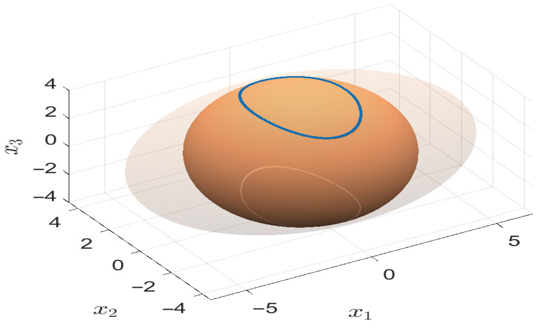
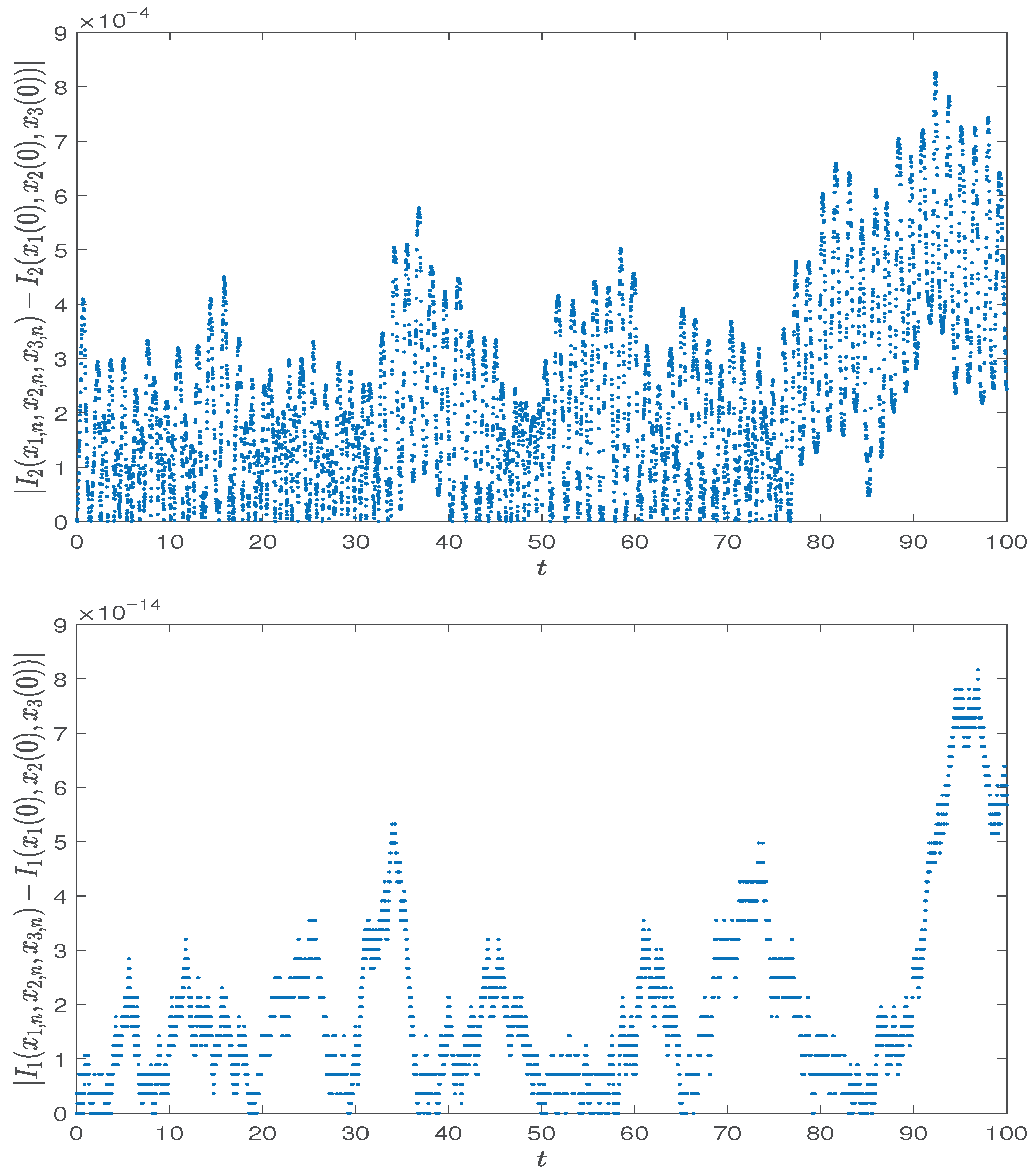
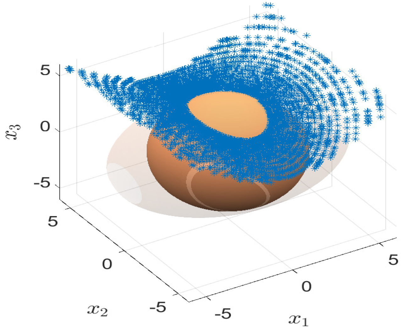
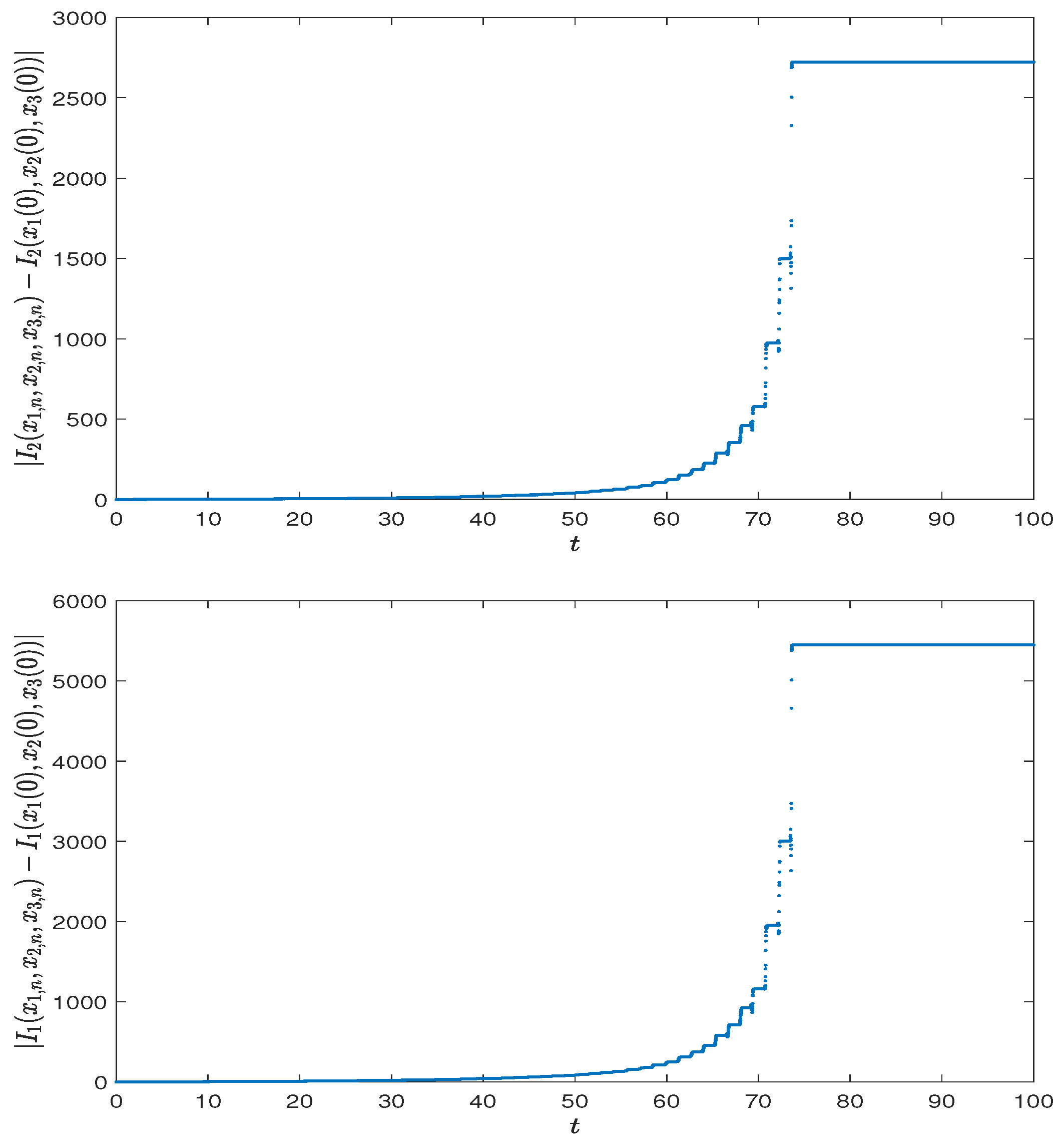
Let the parameters c 1 = 1 , c 2 = 0.1 , R = 4 , I 1 = 2 , I 2 = 1 , I 3 = 2 / 3 , the initial values x 1 ( 0 ) = R cos ( 1.1 ) , x 2 ( 0 ) = 0 , x 3 ( 0 ) = R sin ( 1.1 ) , the time interval t [ 0 , 100 ] and the step size h = 0.01 . We choose the underlying numerical method as the Milstein method and display one numerical sample path and the errors in conserved quantities of the stochastic projection method in Equation (10) in Figure 1 and Figure 2. One numerical sample path and the errors in conserved quantities of the Milstein method are displayed in Figure 3 and Figure 4. It is shown that the stochastic projection method in Equation (10) can preserve the conserved quantities and keep the numerical solution evolving on the correct manifold, while the underlying method can not.
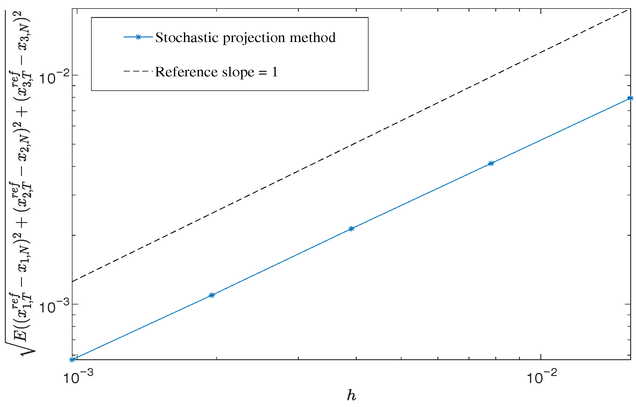
In Figure 5, the mean-square error of the numerical solution, which is estimated as the mean square sample error at the terminal time T = 1 over 1000 different discretized sample paths, is displayed in a log-log plot. For each numerical sample path, the stochastic projection method is applied with five different step sizes: h = 2 5 , 2 6 , 2 7 , 2 8 , 2 9 , and the reference solutions are obtained by the Milstein method with small step size h = 2 15 . As we can see, the stochastic projection method in Equation (10) has the same mean-square convergence order as the Milstein method.

5.2. Stochastic Pendulum Problem

In this example, we consider the stochastic pendulum problem in Cartesian coordinates,
d q 1 ( t ) q 2 ( t ) p 1 ( t ) p 2 ( t ) = p 1 ( t ) p 2 ( t ) q 1 ( t ) μ 1 q 2 ( t ) μ ( d t + c d W ( t ) ) , t [ 0 , T ] ,
where c is some constant and μ = ( p 1 2 + p 2 2 q 2 ) / ( q 1 2 + q 2 2 ) represents the tension on the rob such that the distance between the pendulum and the original maintains. Equation (26) is a SDE defined on the manifold
M = { ( q , p ) I ( q ) = 0 , I ( q ) T H p ( p , q ) = 0 } ,
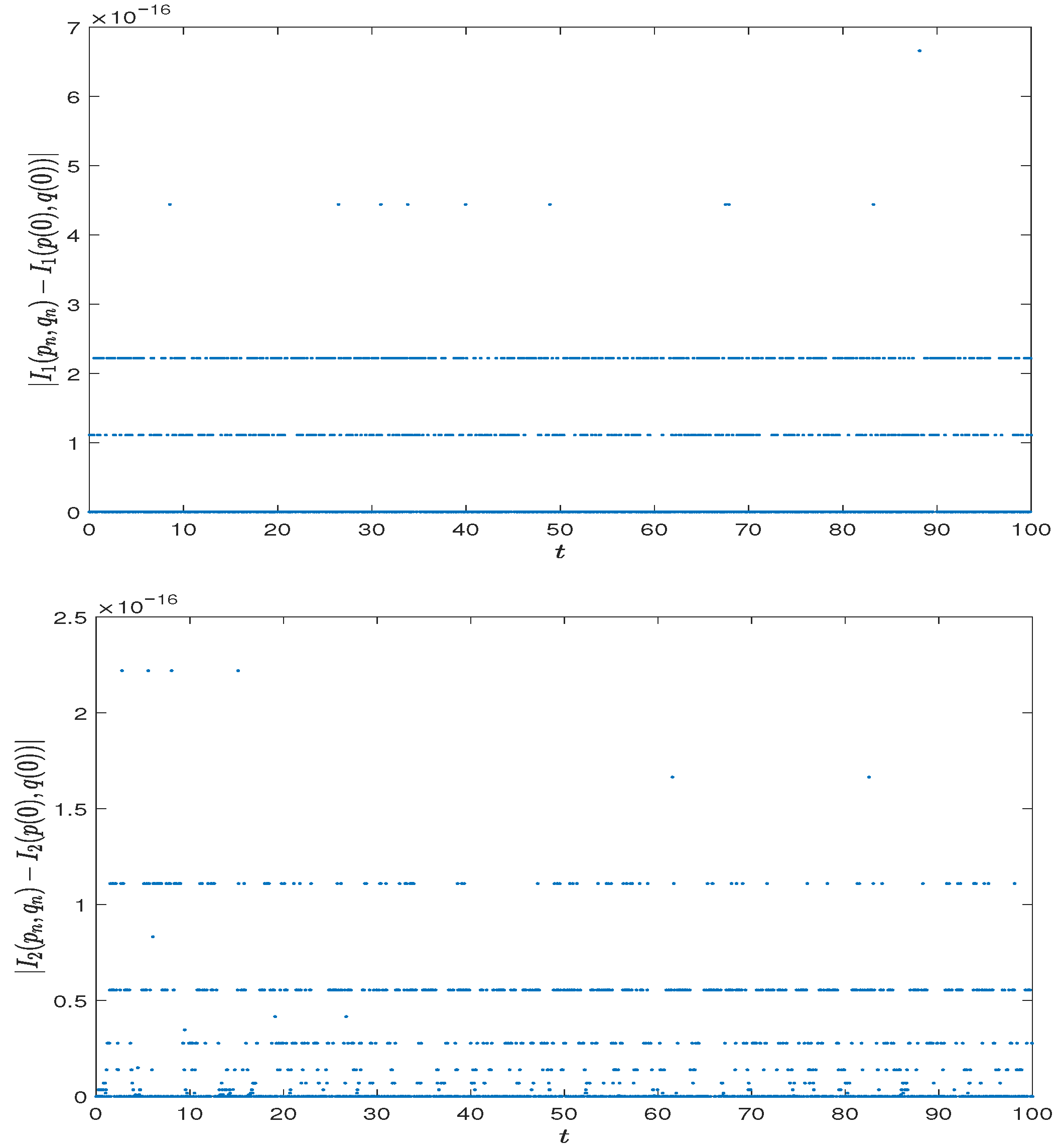
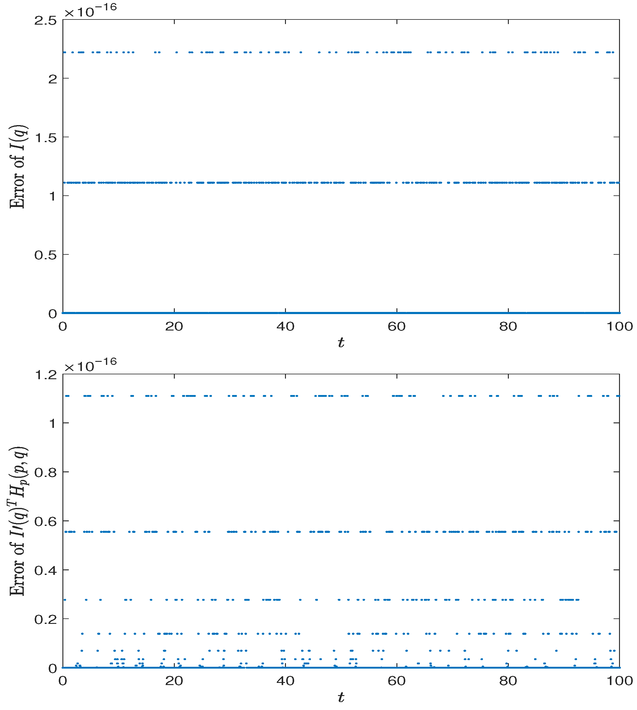
where I ( q ) = q 1 2 + q 2 2 1 is the constraint which represents the length of the massless rod is 1 and H ( p , q ) = ( p 1 2 + p 2 2 ) / 2 + q 2 is the sum of the kinetic and potential energies.
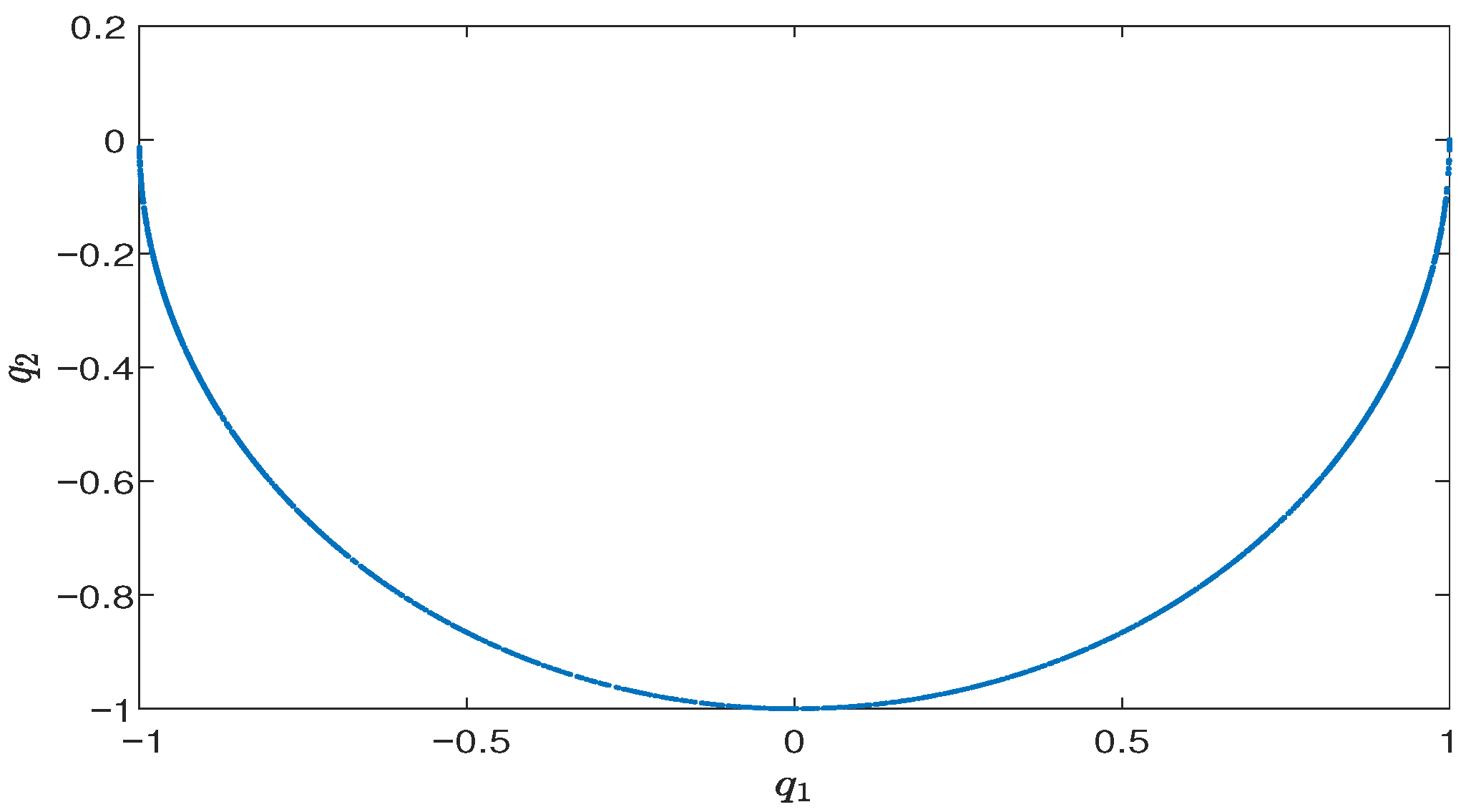
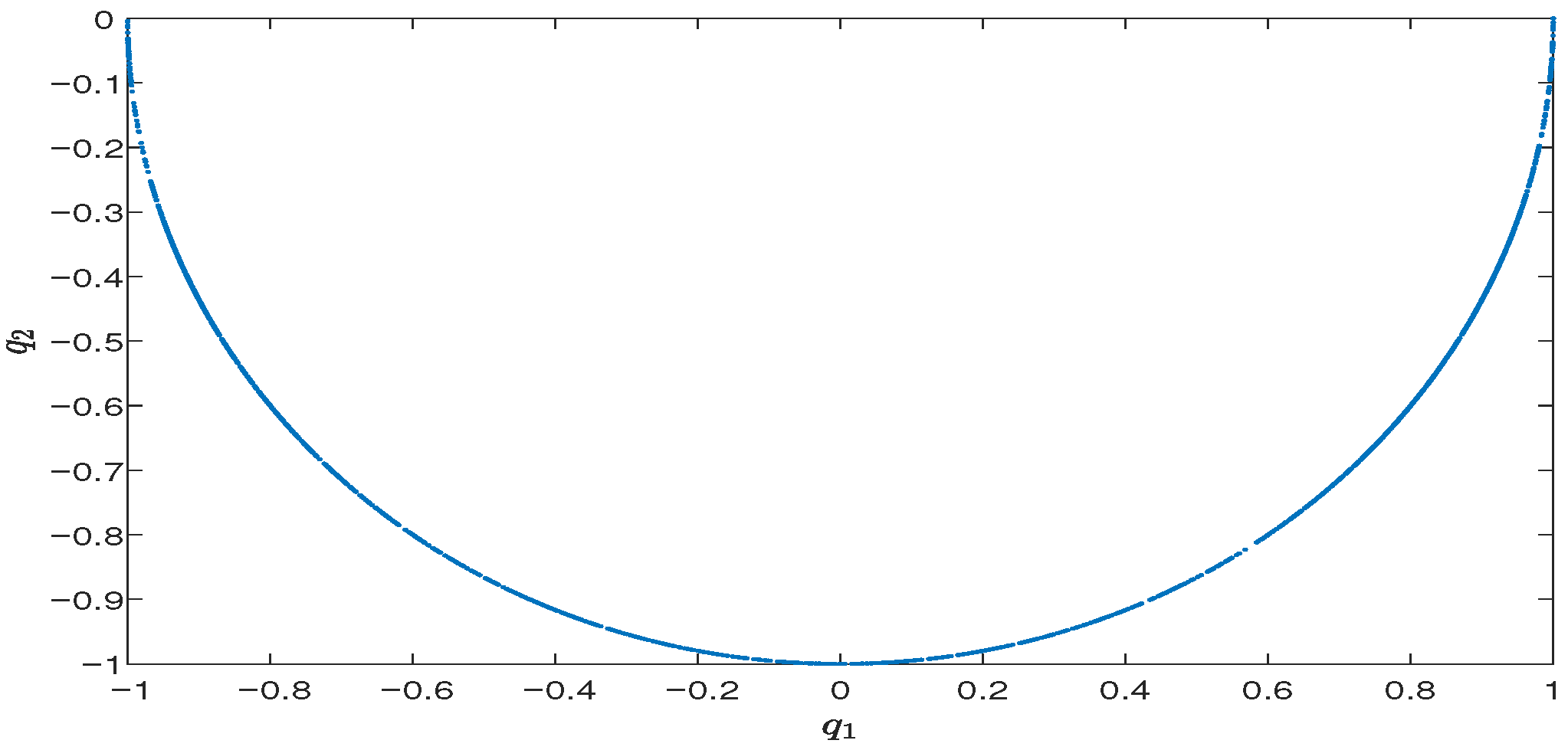
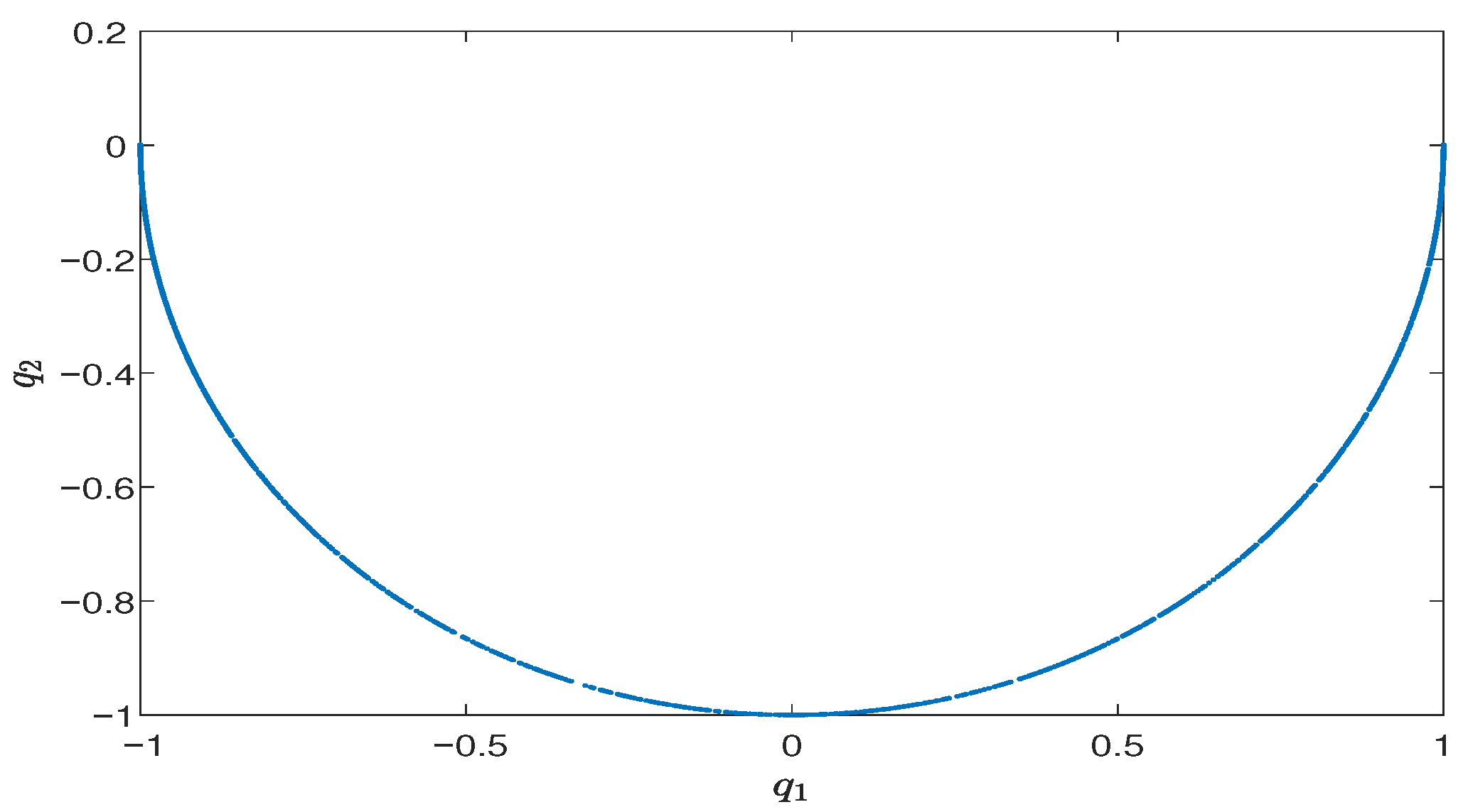
Here, we choose the stochastic mid-point method as the underlying method of method in Equation (19) based on tangent space parametrization in Equation (17). The parameter and initial values are chosen as c = 0.5 , p 1 ( 0 ) = 0 , p 2 ( 0 ) = 0 , q 1 ( 0 ) = 1 , q 2 ( 0 ) = 0 , T = 100 and h = 0.05 .
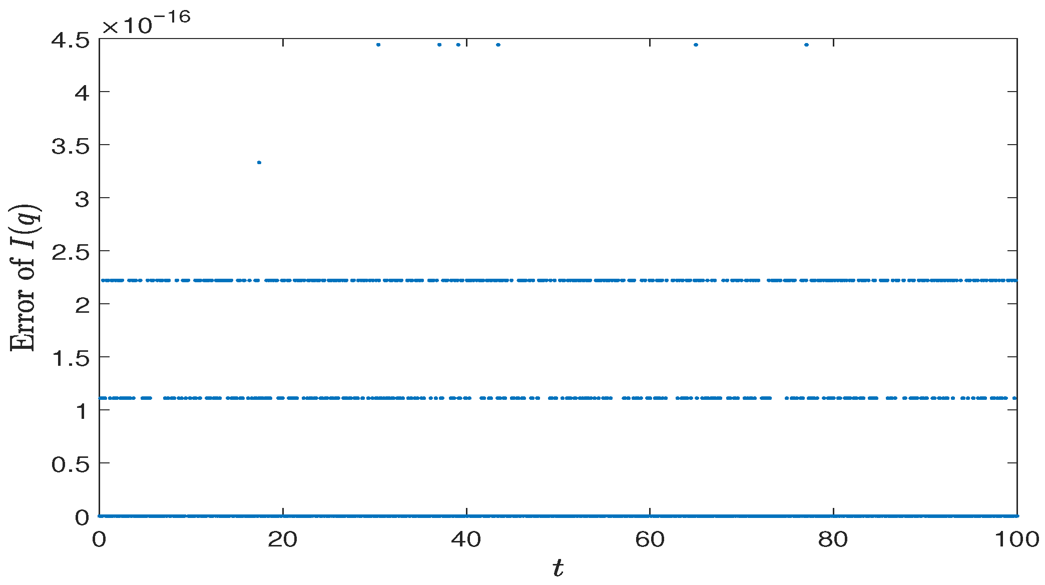
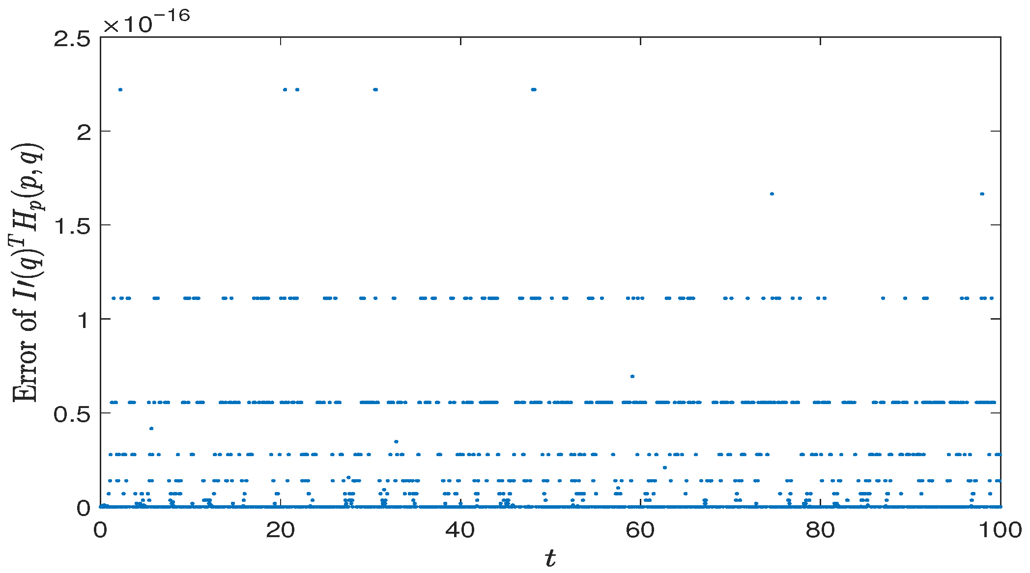
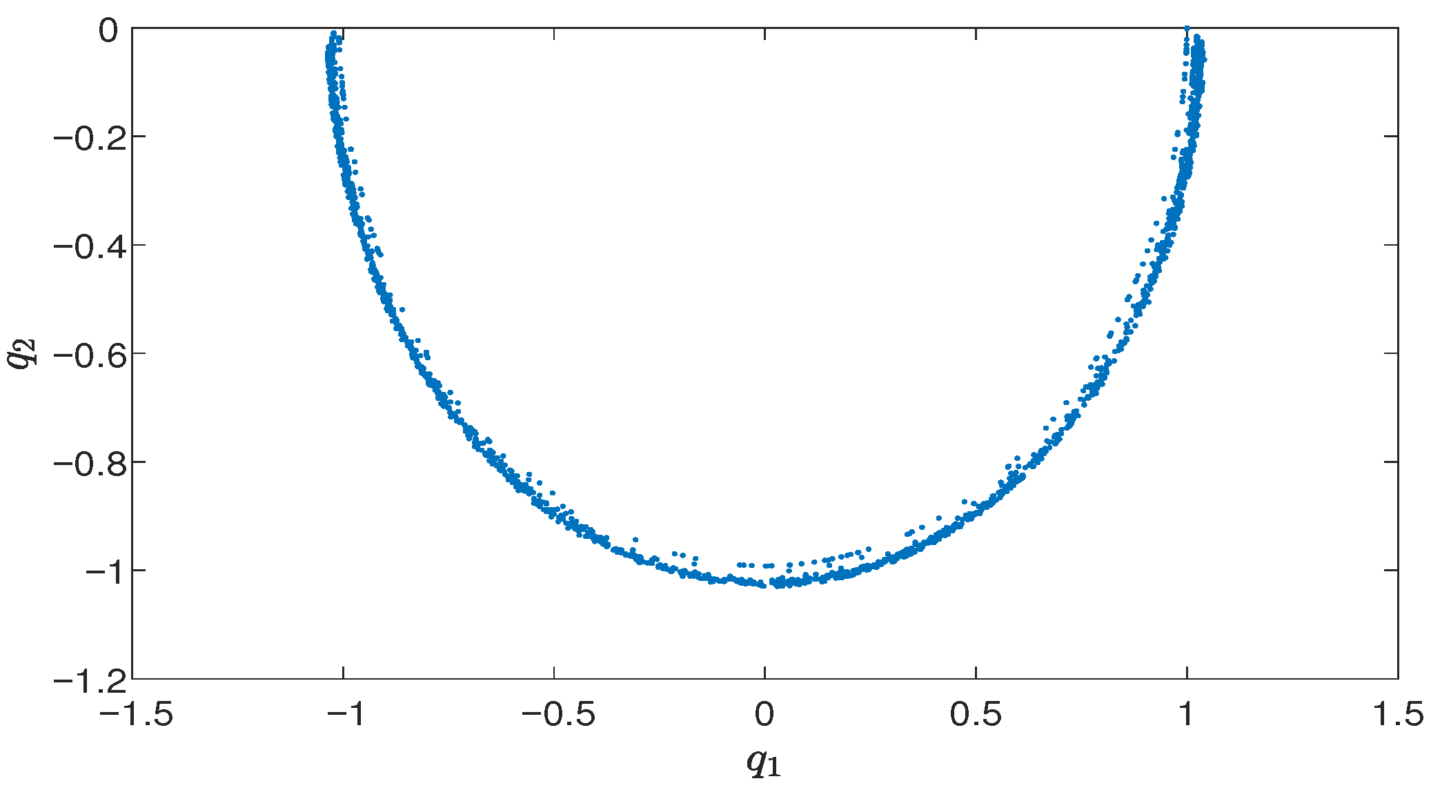
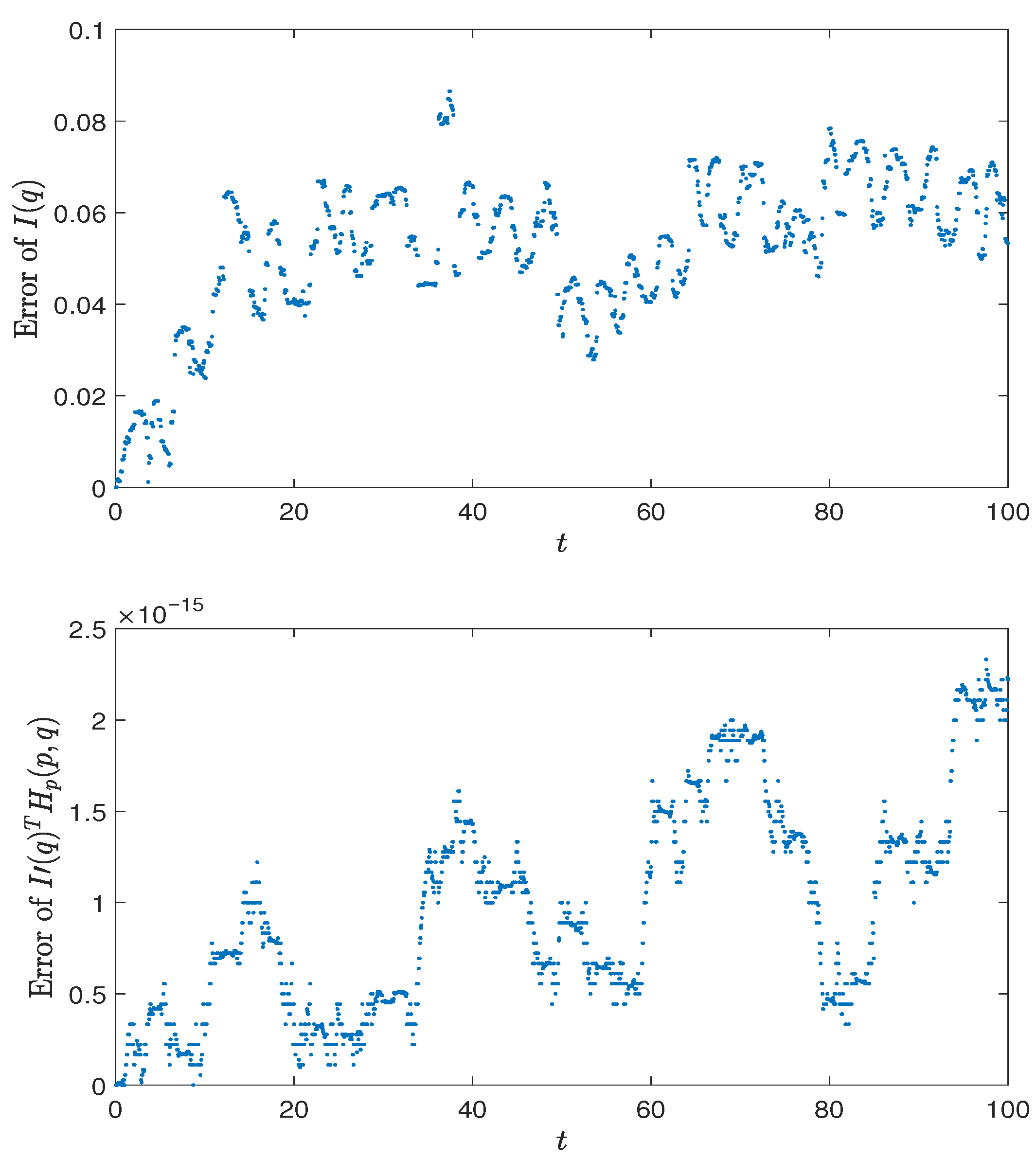
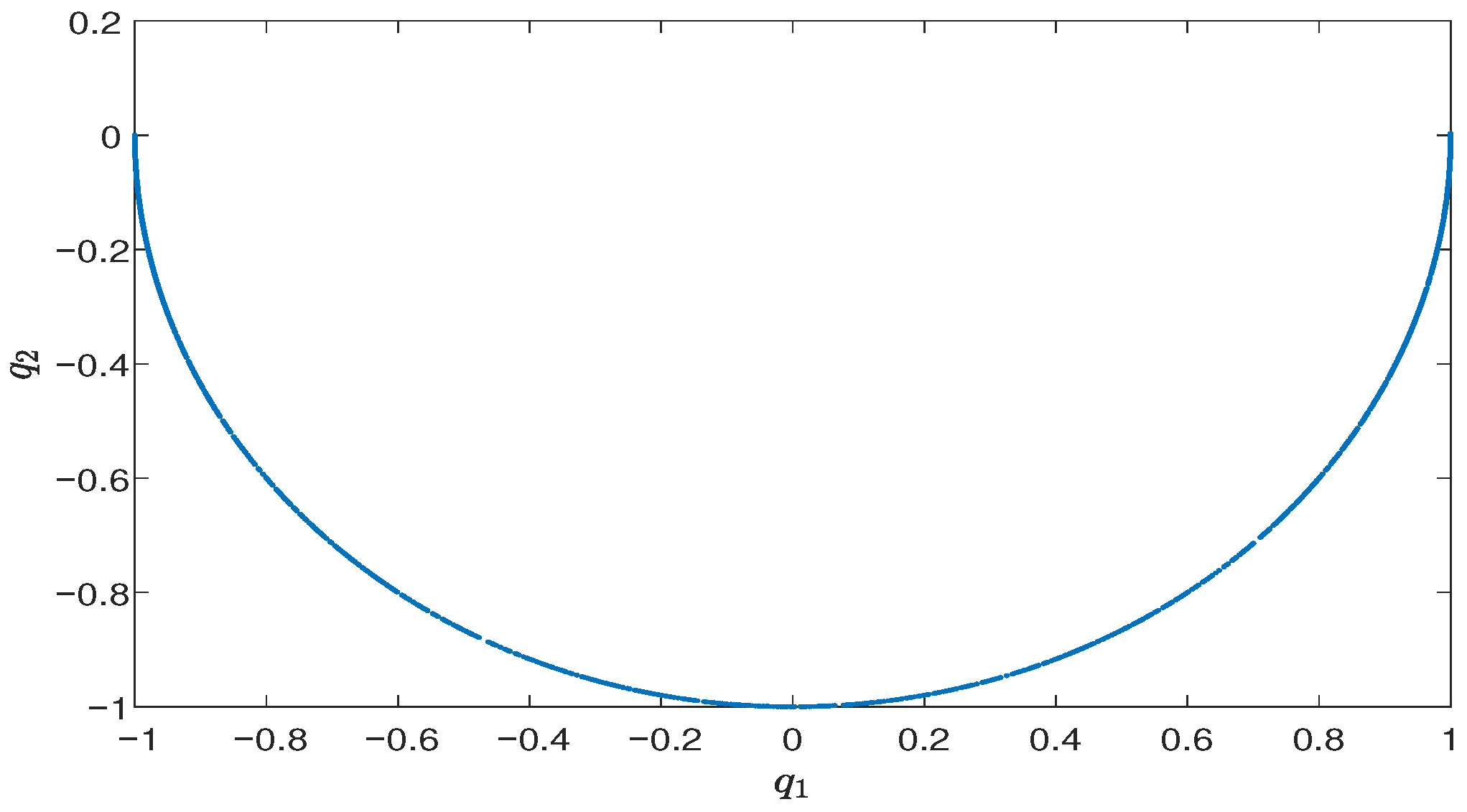
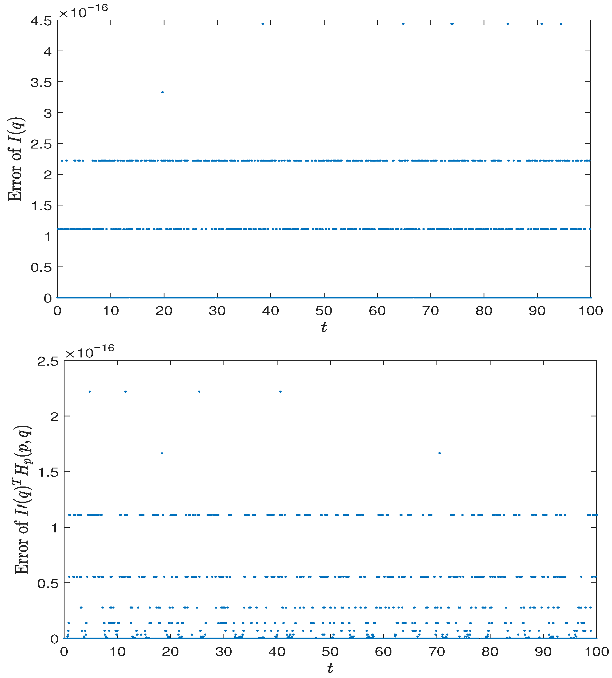
Firstly, we display a numerical sample path and the errors in I 1 = I ( q ) and I 2 = I ( q ) T H p ( p , q ) of method in Equation (19) in Figure 6 and Figure 7. The numerical sample path and the errors in I 1 and I 2 of the stochastic mid-point method are displayed in Figure 8 and Figure 9. As we can see, Equation (19) preserves both conserved quantities and simulates the solution on the manifold correctly.
Secondly, we compare Equation (19) with the standard stochastic linear projection method [13]. The standard stochastic linear projection method is applied to Equation (26) with the same parameter, initial values, h and T. Figure 10 and Figure 11 show that the standard stochastic linear projection method can also simulate the exact solution correctly; however, the CPU time it costs is 6.04 s, while Equation (19) costs 4.04 s. To compare the two numerical methods proposed in this paper, the stochastic projection method in Equation (10) is also used to solve Equation (26) with the same settings. The numerical sample path and the errors in I 1 and I 2 are displayed in Figure 12 and Figure 13, and the cost CPU time is 5.96 s.
Finally, we illustrate that the choice of local coordinates is not unique. For the stochastic pendulum problem in Equation (26), there is a typical choice of local coordinates, which is the polar coordinates. After taking the coordinates transform q 1 = sin ( θ ) , q 2 = cos ( θ ) , p 1 = ω cos ( θ ) and p 2 = ω sin ( θ ) , Equation (26) is transformed into a much simpler case
d θ = ω ( d t + c d W ( t ) ) , t [ 0 , T ] , d ω = sin ( θ ) ( d t + c d W ( t ) ) , t [ 0 , T ] .
Figure 14 and Figure 15 display the numerical sample path and errors in I 1 and I 2 of Equation (19) based on the polar coordinates. It is shown that one can more easily obtain an efficient numerical method that preserves multiple conserved quantities, by appropriately selecting the local coordinates for different problems. In this example, the conserved quantity errors of Equation (19) based on the polar coordinates are smaller than those of Equation (19) based on tangent space parametrization.

5.3. Stochastic Cyclic Lotka–Volterra System

Consider the three-dimensional SDE in the Stratonovich sense called the stochastic cyclic Lotka–Volterra system, which models three species competing in a chaotic environment,
d x ( t ) y ( t ) z ( t ) = x ( t ) ( z ( t ) y ( t ) ) y ( t ) ( x ( t ) z ( t ) ) z ( t ) ( y ( t ) x ( t ) ) ( d t + c d W ( t ) ) , t [ 0 , T ] ,
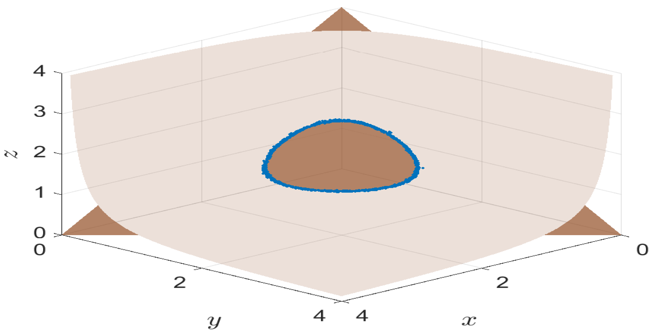
where the parameters and initial values are c = 0.5 , x ( 0 ) = 1 , y ( 0 ) = 2 , z ( 0 ) = 1 . It is easy to verify that functions I 1 ( x , y , z ) = x + y + z and I 2 ( x , y , z ) = x y z are conserved quantities of Equation (28). Thus, the exact flow evolves on the manifold
M = { ( x , y , z ) I 1 ( x , y , z ) = x + y + z = const , I 2 ( x , y , z ) = x y z = const } ,
which represents the intersection of a surface and a flat in R 3 .
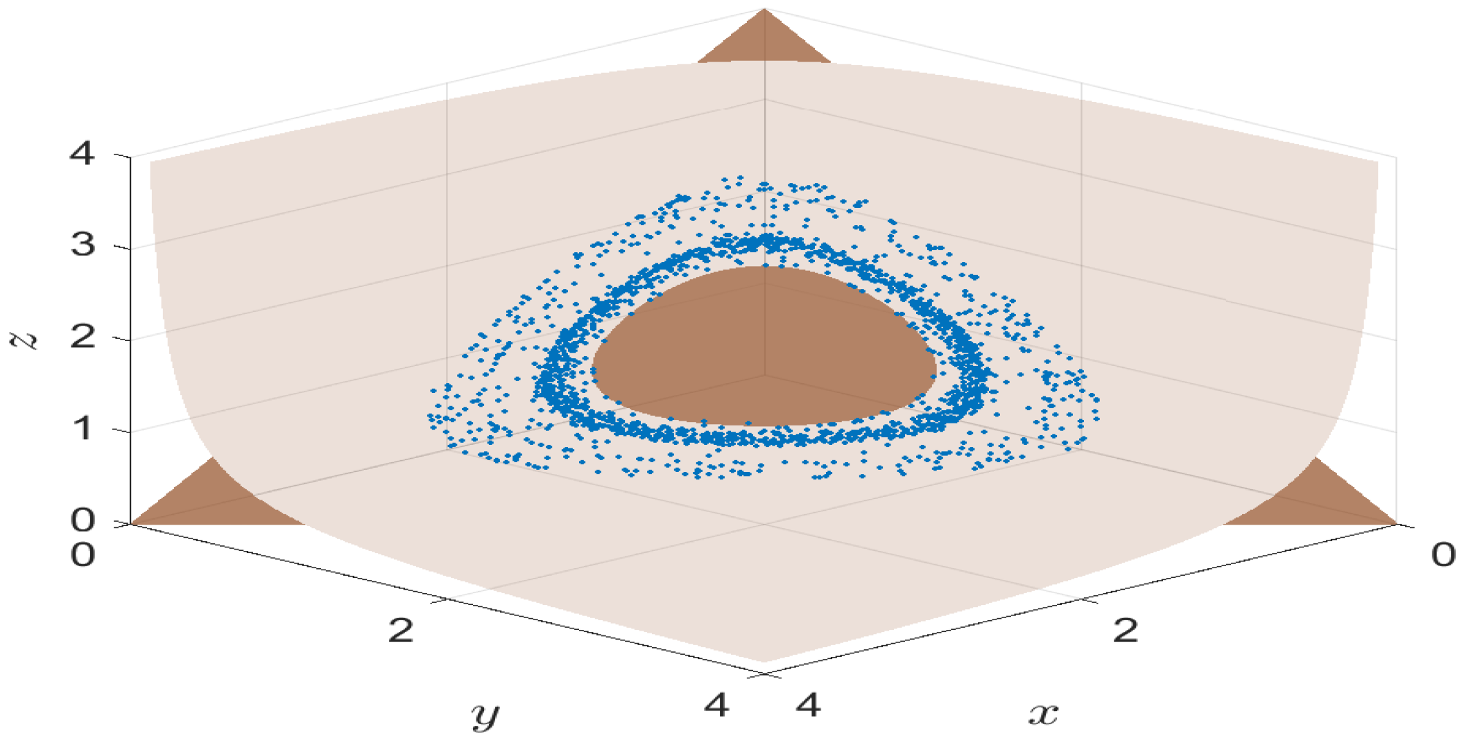
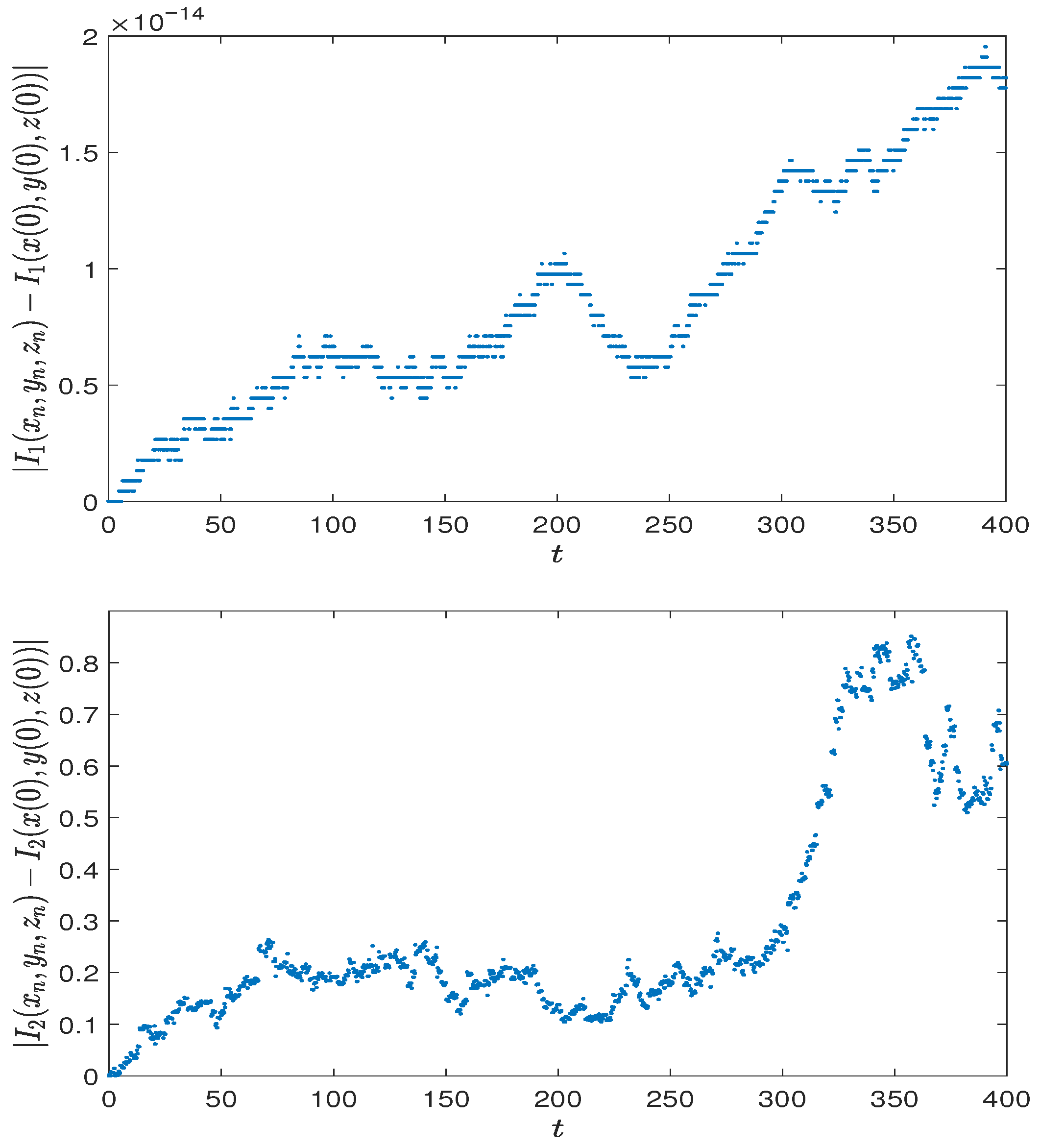
In this example, we show the effectiveness of the strategy proposed in Section 4. Let
I ( x ) = I 1 ( x , y , z ) I 1 ( x ( 0 ) , y ( 0 ) , z ( 0 ) ) 2 + I 2 ( x , y , z ) I 2 ( x ( 0 ) , y ( 0 ) , z ( 0 ) ) 2 .
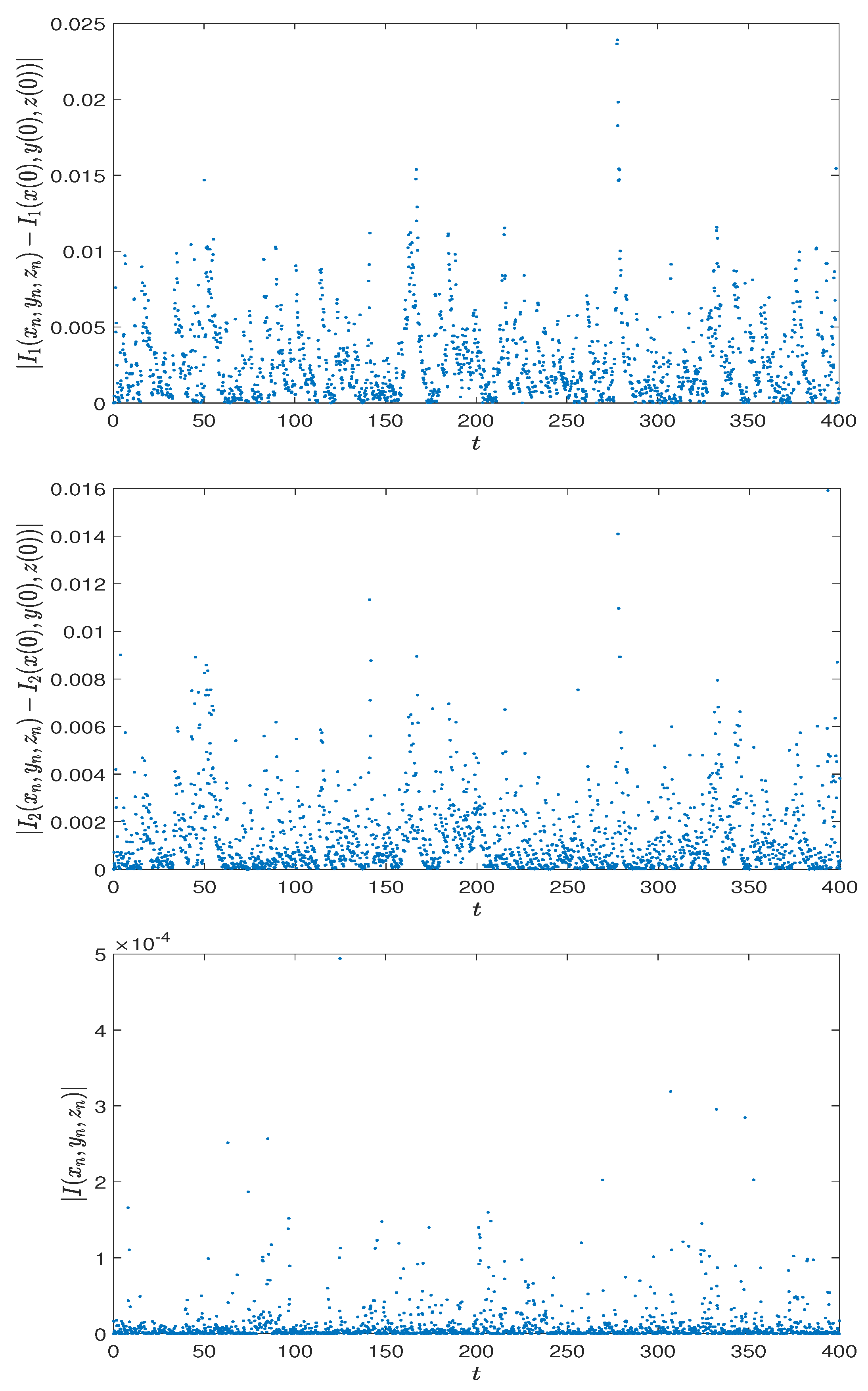
Set T = 400 and h = 0.2 and regard Equation (28) as a SDE with a single conserved quantity I. We choose the stochastic mid-point method as the underlying method, and apply the standard stochastic linear projection method [13] to solve Equation (28) with a single conserved quantity Equation (29). Figure 16, Figure 17, Figure 18 and Figure 19 display one numerical sample path and the errors in conserved quantities I 1 , I 2 and I of the stochastic mid-point method and the standard stochastic linear projection method, respectively. As we can see, the standard stochastic linear projection method with a single conserved quantity Equation (29) provides a more precise numerical solution since errors in both I 1 and I 2 are controlled within magnitude O ( h 2 ) .
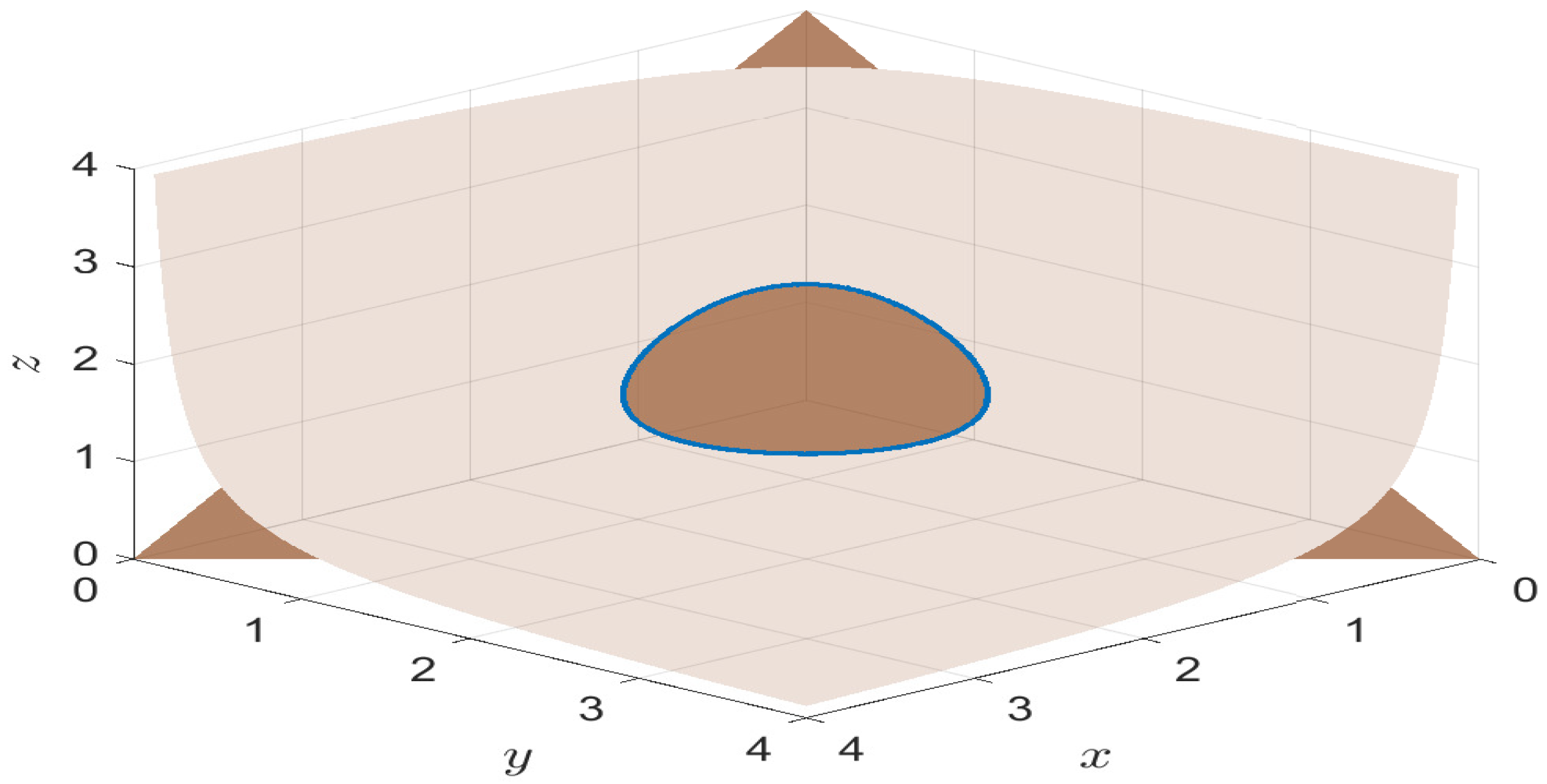
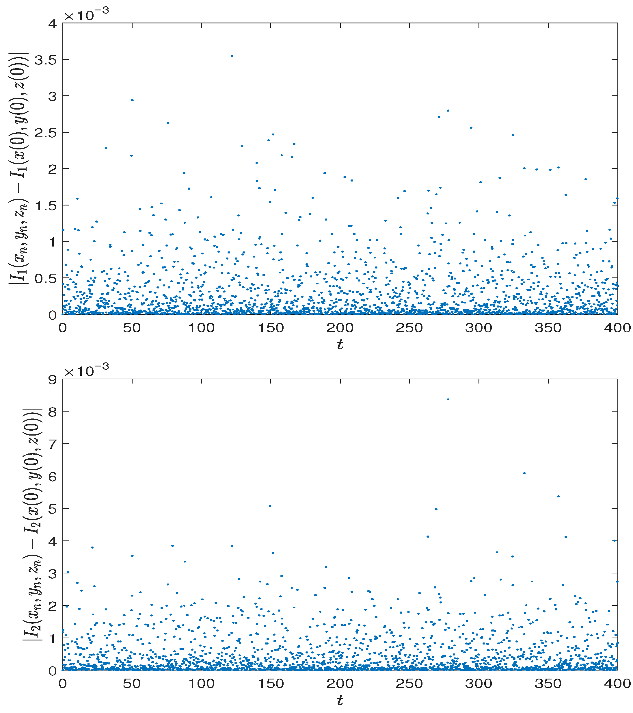
To illustrate the effectiveness of the simplified strategy, we applied the standard stochastic linear projection method to solve Equation (28) with two conserved quantities, a numerical sample path and the errors in conserved quantities I 1 and I 2 are shown in Figure 20 and Figure 21. In this case, a more accurate numerical solution is provided, and the errors in conserved quantities I 1 and I 2 are smaller. However, the CPU time for this case is 11.21 s, while the standard stochastic linear projection method with a single conserved quantity Equation (29) costs 9.13 s.

6. Discussion and Conclusions

Discussion

This study proposed the following two novel projection-based methods for preserving multiple conserved quantities in SDEs:
  • Discrete Tangent Space Projection:
    Advantages: This method is general-purpose and does not require explicit knowledge of the manifold geometry. It projects increments onto a discrete tangent space, ensuring exact conservation by construction. It is also symmetric if the underlying scheme and discrete gradient are symmetric (Remark 1).
    Disadvantages: The projection step involves a QR decomposition (Equation (12)), which can be computationally expensive for high-dimensional systems or large M (number of invariants). It may also suffer from numerical stiffness if the discrete gradients are ill-conditioned.
  • Local Coordinates-Based Method:
    Advantages: By solving the SDE on a local coordinate chart, this method inherently restricts the solution to the manifold. It can be more efficient when a natural parametrization exists (e.g., polar coordinates for the pendulum, as in Section 5.2).
    Disadvantages: Its efficiency depends heavily on the choice of local coordinates. For complex manifolds, finding a global or stable parametrization may be challenging. It also requires computing the orthonormal basis of the tangent space (Remark 2), which adds overhead.
A simplified strategy was also introduced to balance accuracy and computational cost (Section 4), but sacrifices exact conservation. This trade-off may not be acceptable for systems where small drifts lead to qualitative errors. However, the numerical experiments focused on low-dimensional systems (e.g., 3D rigid body). The performance of both methods in high-dimensional settings (e.g., molecular dynamics) remains untested and may require optimizations.

Author Contributions

Conceptualization, Z.W. and X.D.; methodology, X.L. and Z.W.; software, X.L. and Z.W.; validation, X.L. and X.D.; formal analysis, Z.W.; investigation, X.L.; resources, X.L.; data curation, X.L.; writing—original draft preparation, Z.W.; writing—review and editing, X.L.; visualization, X.L.; supervision, X.D.; project administration, X.D.; funding acquisition, Z.W. All authors have read and agreed to the published version of the manuscript.

Funding

This work was funded by the National Natural Science Foundation of China (No. 12401519) and the Natural Science Foundation of Shandong Province of China (No. ZR2022QA051).

Data Availability Statement

The original contributions presented in this study are included in the article. Further inquiries can be directed to the corresponding author.

Conflicts of Interest

The authors declare no conflicts of interest.

References

  1. Mao, X. Stochastic Differential Equations and Applications; Horwood Publishing: Chichester, UK, 2007. [Google Scholar]
  2. Milstein, G.N. Numerical Integration of Stochastic Differential Equations; Kluwer Academic Publishers: Dordrecht, The Netherlands, 1995. [Google Scholar]
  3. Milstein, G.N.; Repin, Y.M.; Tretyakov, M.V. Numerical methods for stochastic systems preserving symplectic structure. SIAM J. Numer. Anal. 2002, 40, 1583–1604. [Google Scholar] [CrossRef]
  4. Han, M.; Ma, Q.; Ding, X. High-order stochastic symplectic partitioned Runge-Kutta methods for stochastic Hamiltonian systems with additive noise. Appl. Math. Comput. 2019, 346, 575–593. [Google Scholar] [CrossRef]
  5. Zhang, L.; Ji, L. Stochastic multi-symplectic Runge-Kutta methods for stochastic Hamiltonian PDEs. Appl. Numer. Math. 2019, 135, 396–406. [Google Scholar] [CrossRef]
  6. D’Ambrosio, R.; Di Giovacchino, S. Strong backward error analysis of symplectic integrators for stochastic Hamiltonian systems. Appl. Math. Comput. 2024, 467, 128488. [Google Scholar] [CrossRef]
  7. Wang, L.; Wang, P.; Cao, Y. Numerical methods preserving multiple Hamiltonians for stochastic Poisson systems. Discret. Contin. Dyn. Syst.-Ser. S 2022, 15, 819. [Google Scholar] [CrossRef]
  8. Armstrong, J.; King, T. Curved schemes for stochastic differential equations on, or near, manifolds. Proc. R. Soc. A 2022, 478, 20210785. [Google Scholar] [CrossRef]
  9. Bréhier, C.É.; Cohen, D.; Komori, Y. Stochastic conformal integrators for linearly damped stochastic poisson systems. arXiv 2025, arXiv:2503.01540. [Google Scholar] [CrossRef]
  10. Malham, S.J.A.; Wiese, A. Stochastic Lie group integrators. SIAM J. Sci. Comput. 2008, 30, 597–617. [Google Scholar] [CrossRef][Green Version]
  11. Wang, Z.; Ma, Q.; Yao, Z.; Ding, X. The Magnus expansion for stochastic differential equations. J. Nonlinear Sci. 2020, 30, 419–447. [Google Scholar] [CrossRef]
  12. Hong, J.; Zhai, S.; Zhang, J. Discrete gradient approach to stochastic differential equations with a conserved quantity. SIAM J. Numer. Anal. 2011, 49, 2017–2038. [Google Scholar] [CrossRef]
  13. Zhou, W.; Zhang, L.; Hong, J.; Song, S. Projection methods for stochastic differential equations with conserved quantities. BIT Numer. Math. 2016, 56, 1497–1518. [Google Scholar] [CrossRef]
  14. Chen, C.; Hong, J.; Jin, D. Modified averaged vector field methods preserving multiple invariants for conservative stochastic differential equations. BIT Numer. Math. 2020, 60, 917–957. [Google Scholar] [CrossRef]
  15. Dahlby, M.; Owren, B.; Yaguchi, T. Preserving multiple first integrals by discrete gradients. J. Phys. A Math. Theor. 2010, 44, 1651–1659. [Google Scholar] [CrossRef]
  16. Wang, Z.; Wang, C.; Ma, Q.; Ding, X. Numerical simulations for stochastic differential equations on manifolds by stochastic symmetric projection method. Phys. A Stat. Mech. Its Appl. 2020, 541, 123305. [Google Scholar] [CrossRef]
  17. Hairer, E.; Lubich, C.; Wanner, G. Geometric Numerical Integration: Structure-Preserving Algorithms for Ordinary Differential Equations; Springer Science & Business Media: Berlin, Germany, 2006. [Google Scholar]
Figure 1. Numerical sample path by the stochastic projection method in Equation (10) for solving Equation (23).
Mathematics 13 03614 g001
Figure 2. Errors of I 1 (top) and I 2 (bottom) by the stochastic projection method in Equation (10) for solving Equation (23).
Mathematics 13 03614 g002
Figure 3. Numerical sample path by Milstein method for solving Equation (23).
Mathematics 13 03614 g003
Figure 4. Errors of I 1 (top) and I 2 (bottom) by Milstein method for solving Equation (23).
Mathematics 13 03614 g004
Figure 5. The convergence rate of stochastic projection method in Equation (10) for solving Equation (23).
Mathematics 13 03614 g005
Figure 6. Numerical sample path by Equation (19) based on tangent space parametrization in Equation (17) for solving Equation (26).
Mathematics 13 03614 g006
Figure 7. Errors of I 1 and I 2 by Equation (19) based on tangent space parametrization in Equation (17) for solving Equation (26).
Mathematics 13 03614 g007aMathematics 13 03614 g007b
Figure 8. Numerical sample path by the stochastic mid-point method for solving Equation (26).
Mathematics 13 03614 g008
Figure 9. Errors of I 1 and I 2 by the stochastic mid-point method for solving Equation (26).
Mathematics 13 03614 g009
Figure 10. Numerical sample path by the standard stochastic linear projection method for solving Equation (26).
Mathematics 13 03614 g010
Figure 11. Errors of I 1 and I 2 by the standard stochastic linear projection method for solving Equation (26).
Mathematics 13 03614 g011
Figure 12. Numerical sample path by the stochastic projection Equation (10) for solving Equation (26).
Mathematics 13 03614 g012
Figure 13. Errors of I 1 and I 2 by the stochastic projection Equation (10) for solving Equation (26).
Mathematics 13 03614 g013
Figure 14. Numerical sample path by Equation (19) based on polar coordinate for solving Equation (26).
Mathematics 13 03614 g014
Figure 15. Errors of I 1 and I 2 by Equation (19) based on polar coordinate for solving Equation (26).
Mathematics 13 03614 g015
Figure 16. Numerical sample path by the stochastic mid-point method for solving Equation (28).
Mathematics 13 03614 g016
Figure 17. Errors of I 1 and I 2 by the stochastic mid-point method for solving Equation (28).
Mathematics 13 03614 g017
Figure 18. Numerical sample path by the standard stochastic linear projection method based on single conserved quantity Equation (29) for solving Equation (28).
Mathematics 13 03614 g018
Figure 19. Errors of I 1 , I 2 and I by the standard stochastic linear projection method based on single conserved quantity Equation (29) for solving Equation (28).
Mathematics 13 03614 g019
Figure 20. Numerical sample path by the standard stochastic linear projection method based on two conserved quantities I 1 and I 2 for solving Equation (28).
Mathematics 13 03614 g020
Figure 21. Errors of I 1 and I 2 by the standard stochastic linear projection method based on two conserved quantities I 1 and I 2 for solving Equation (28).
Mathematics 13 03614 g021
Disclaimer/Publisher’s Note: The statements, opinions and data contained in all publications are solely those of the individual author(s) and contributor(s) and not of MDPI and/or the editor(s). MDPI and/or the editor(s) disclaim responsibility for any injury to people or property resulting from any ideas, methods, instructions or products referred to in the content.