Abstract
This study examines the exposure of the U.S. insurance sector to climate-related risks using a two-step approach combining factor modeling and Extreme Value Theory. The analysis first constructs a climate risk factor from transition-sensitive sectors and estimates its impact on the SPDR S&P Insurance ETF using a standard factor model. The resulting residual, termed Insurance Climate Risk, isolates climate-driven excess returns by controlling for market-wide effects. To assess the sector’s sensitivity to extreme events, the study applies both the Peaks Over Threshold method using the Generalized Pareto Distribution and the Block Maxima Method using the Generalized Extreme Value distribution. The findings reveal statistically significant climate sensitivity, especially in daily and weekly data, and confirm the presence of heavy tails in the loss distribution. VaR and CVaR estimates indicate heightened risk over longer horizons and under block maxima modeling. Notably, peak over threshold daily returns yield a 95% VaR of 1.33% and CVaR of 2.28%, while block maxima CVaR exceeds 5%. These results show the importance of incorporating tail-risk-aware metrics in insurance risk management and highlight the growing influence of climate-related financial shocks.
Keywords:
Extreme Value Theorem; factor model; Value at Risk; Conditional Value at Risk; Generalized Pareto Distribution; Generalized Extreme Value; peak over threshold; Block Maxima MSC:
60G70; 91G70; 62P05
1. Introduction
Climate-related risks in financial markets have become an increasingly important focus in recent decades, driven by the economic instability posed by the acute and chronic impacts of climate on assets and insurance costs [1,2]. Although climate risks are widely recognized by most financial institutions, investors, and policymakers, effectively incorporating and estimating these risks poses a complex challenge in decision making. This complexity often leads to unexpected financial losses. These challenges become even harder as investors and financial institutions also need to meet the growing demands of stakeholders to include environmental, social, and governance (ESG) factors in their investment strategies. However, determining the true ESG rating of a company has faced substantial uncertainty due to different ratings from different agencies [3].
Climate change poses significant challenges to the stability of the financial system, with the insurance sector occupying a particularly vulnerable position. Since they play a leading role in shifting and managing climate-related losses, as they provide financial protection against climate-related losses [4]. Insurers face both physical risks that arise from extreme weather events, such as floods, wildfires, droughts, and rising sea levels. For example, ref. [5] analyzes the impact of hurricanes on insurance stock returns in the United States, finding that high-category hurricanes are associated with negative abnormal returns for insurance stocks, with the severity of hurricane damage showing a statistically significant negative correlation with stock performance. Physical risks also have significant implications for asset pricing and insurance markets. Ref. [6] highlights that the assessment of climate risks at the asset level is critical to understanding adaptation and financial losses from extreme events. Similarly, ref. [7] provided evidence that regions with higher exposure to heat stress face increased spreads of bond yields and higher expected returns of equity.
Transition risk, in contrast to physical risk, arises from changes in policy, technology, and consumer preferences toward low-carbon alternatives, which can lead to significant devaluation of carbon-intensive assets [8]. In recent decades, the number of climate-related policies adopted globally has increased significantly. As governments strengthen their commitment to reducing carbon emissions, financial markets are beginning to price transition risks more [9,10]. For example, the implementation of policies such as the Paris Agreement has resulted in credit rating downgrades for firms highly exposed to transition risks, with European firms being more affected than US firms, reflecting differing climate policy expectations [11,12]. Furthermore, insurers are increasingly responding to regulatory pressure and the growing recognition of transition risks in the market [13,14]. Although many experts have expressed concerns that current prices do not fully reflect these risks [1,15,16,17]. Ref. [18] shows that delays in implementing climate transition policies can themselves amplify long-term financial tail risks, highlighting the importance of timely mitigation strategies. These findings suggest a growing recognition of transition risks in the financial market, as the financial impacts of shifting toward a low-carbon economy are increasingly reflected in asset valuations and insurance sector dynamics.
As climate risks, both physical and transition-related, continue to affect asset pricing and insurance markets, there is a growing need for effective tools to measure and manage these risks; as such, traditional tools such as Value at Risk (VaR) and Conditional Value at Risk (CVaR) play a critical role. VaR has been the most popular risk measure in recent decades and was popularized by JP Morgan’s release of the RiskMetrics framework in 1996 [19] and has played an important role in risk management, risk measurement, financial control, and financial reporting. VaR is a quantile-based measure , which measures the excess market risk associated with a portfolio by determining how much the value of the portfolio could decline with % probability over a certain period as a result of market price or rate changes. However, VaR has well-known shortcomings; it assumes normal market conditions, underestimates tail risks, and provides no information about losses beyond its threshold for excess risks. In addition, VaR is nonsubadditive [20,21], that is, if there exist portfolios A and B with losses and , there are cases where the VaR of the total portfolio is higher than the sum of the VaR of individual portfolios, such that , so diversification can fail under VaR. For these reasons, the study complements VaR with CVaR (Expected Shortfall), which summarizes the average loss in the tail beyond .
To improve VaR accuracy, particularly under volatile conditions, since most financial impacts often exhibit non-linear patterns, that is, a period of high volatility is highly predicted to be followed by high volatility and vice versa, advanced models such as Generalized Autoregressive Conditional Heteroskedasticity (GARCH) have been employed [22]. Although GARCH excels at modeling volatility clustering, its assumption of normality in residuals often underestimates tail risks due to fat tails and excess kurtosis observed in real-world financial returns [23,24].
Likewise, traditional VaR models struggle to capture the complex and uncertain nature of climate change in the insurance sector. Unlike other financial risks, such as credit, interest, and liquidity, climate risks often exhibit longer time horizons, nonlinear impacts, and interdependencies across multiple economic sectors. For insurers, this means that risk measurement must account for rare but severe climate-driven losses, such as those triggered by extreme weather events. Adapting VaR methodologies by integrating climate-sensitive data and Extreme Value Theory (EVT) has therefore become essential [25]. EVT is particularly effective in capturing extreme returns during periods of market stress by focusing on the tail distribution of losses rather than the entire distribution [22,24]. However, one major limitation of EVT is its assumption of independent and identically distributed (i.i.d.) returns, which may not always hold in financial time series. This assumption makes it difficult to apply EVT effectively over extended time horizons, as financial returns tend to exhibit time-varying volatility and clustering, which are ignored by the i.i.d. assumption [22].
To address limitations of both the GARCH and EVT models when applied separately, ref. [22] proposed the GARCH-EVT model, which combines the time-varying volatility of GARCH with the ability of EVT to model extreme events. In this two-stage approach, a GARCH model is used first to model volatility, and then EVT is applied to the residuals to capture tail risk. This two-stage procedure is useful for climate-related risk assessment in the insurance sector, as it accounts for both volatility clustering and the heavy-tailed nature of loss distributions. This in turn provides more reliable short-term risk forecasts [22,23].
Evidence of the existence of excess tail risk has already been discussed in the literature [26]. Refs. [24,27] demonstrates the effectiveness of Univariate Extreme Value Theory in modeling extreme market risk, showing that a dynamic EVT approach based on GARCH (1,1) outperforms traditional GARCH (1,1). In contrast, ref. [28] tests four algorithmic POT thresholds within a GARCH-EVT model on 10 world stock indices (2000–2019) and finds no improvement in VaR accuracy relative to a fixed 95th percentile cutoff. Furthermore, ref. [23] finds that E-GARCH with GED outperforms for 1-day VaR on major equity markets, while conditional EVT performs similarly to GARCH under GED.
However, GARCH-EVT models are primarily effective for short-term forecasting, typically over a few days to weeks. While they perform well in predicting short-term extreme risks, they are less suitable for long-term (quarterly or annual) forecasts. This is because GARCH-EVT models are based on historical data, and financial market conditions can change significantly over longer periods, reducing the predictive accuracy of the model. For long-term predictions, the assumption that volatility and extreme behavior remain consistent can lead to overfitting and misestimation of excess risks [22,24].
In contrast, climate stress tests have emerged as a key tool to better assess these risks [29]. Stress testing focuses on the tails of a loss distribution based on VaR models [30]. Insurers and regulators have started using climate stress tests to evaluate exposures in a wide range of physical and transition risk scenarios [17,31,32]. These scenario-based approaches, including tools such as integrated assessment models (IAMs) [33] and forward-looking frameworks such as CRISK [34], and supervisory methods such as the Pioneers Detection Method [35], help estimate potential capital shortfalls and changes in asset values under different climate pathways. For the insurance sector, this adds an important layer to risk assessment by allowing institutions to plan for slow-building, systemic risks that may not show up in short-term data, such as increasing claims, asset repricing, or regulatory shifts tied to climate policy.
Building on previous work [36], the primary objective of this study is to assess the US insurance sector’s exposure to climate-related financial risks by integrating a factor-based model with extreme value theory. Although GARCH-EVT and other EVT approaches have been applied to financial markets, they typically focus on aggregate indices or individual assets and do not isolate insurance sector-specific climate exposures. In contrast, our study combines a factor-based climate risk model with EVT tail estimation using both the Peaks Over Threshold and Block Maxima Method frameworks, allowing us to capture extreme losses specifically attributable to climate risks in the insurance sector while controlling for broader market movements.
This study addresses a central challenge in climate risk modeling for insurers: linking climate-related losses to other market-wide and sector-specific risks. Because climate risks often exhibit complex interdependencies between sectors such as energy, metals/mining, transportation, and insurance, it is essential to isolate the component of insurer exposure specifically attributable to climate hazards.
This paper makes three key contributions to the financial risk management literature. First, it constructs a climate risk factor by combining returns from climate-sensitive sectors, isolating climate-related losses from general market fluctuations. Second, it applies a factor model to quantify the sensitivity of insurance firm returns to both market and climate factors. Third, it estimates the tail risk of insurance climate losses using both the POT and BMM approaches from EVT to compute VaR and CVaR. By linking factor-model sensitivities with rigorous tail-risk estimation, this study provides an empirically grounded framework for assessing extreme climate-related insurance losses, offering applicable insights for insurers, regulators, and risk managers.
2. Data and Methodology
The analysis begins by constructing a proxy for the climate factor; the study follows the approach of [37], using a linear combination of returns from climate-sensitive sectors and removing common market influences to represent systematic climate risk. This climate factor captures the overall influence of climate risks across key sectors, while accounting for sector-specific fluctuations. To assess the sensitivity of the insurance sector to climate exposure, the study applies a standard linear factor model adapted from [34], including both the market portfolio and a constructed climate factor as explanatory variables. This allows us to separate the portion of insurance sector returns driven by general market conditions from those specifically linked to climate-related risks.
After isolating the climate-specific excess risk component in the insurance sector, the study applies EVT to model the tail behavior of these returns. In this study, we employ both the Peaks Over Threshold (POT) approach, which fits a Generalized Pareto Distribution (GPD) to exceedances above a high threshold, and the Block Maxima method, which models the distribution of extreme returns within fixed intervals using the Generalized Extreme Value (GEV) distribution. By applying these methods to excess returns on climate-adjusted insurance, the analysis calculates VaR and CVaR, providing a detailed measure of the sector’s exposure to extreme climate-driven financial losses. This dual EVT approach allows us to evaluate the sensitivity and consistency of tail risk estimates under different assumptions, offering valuable insights for risk management in the insurance industry.
2.1. Dataset
The focus of this study is to model the climate-related risk exposure of the SPDR S&P Insurance ETF (KIE) by analyzing its financial results and estimating VaR and CVaR over the period January 2007 to December 2024, which contains 4528 daily observations. Historical daily return data are obtained from Yahoo Finance for the S&P 500 index (⌃GSPC) as a proxy for the general market, as well as three sectoral ETFs: the Energy Select Sector SPDR (XLE), the SPDR S&P Metals and Mining ETF (XME), and the SPDR S&P Insurance ETF (KIE). These sector ETFs are selected for their relevance to climate-related risks: XLE and XME represent industries that are particularly sensitive to transition risks due to carbon intensity and regulatory exposure, while KIE reflects the financial sector’s exposure to physical risks. Using these sectors, the article aims to capture both the transition and physical dimensions of climate risk in constructing the climate factor and evaluating its impact on the insurance sector.
Table 1 provides a detailed summary statistic of daily logarithmic returns, including mean, standard deviation, skewness, and kurtosis for each sector. Across all indices, the mean daily return is close to zero, with SPY showing the highest average (0.032%) and XME the lowest (0.004%). XME also shows the highest volatility, with a standard deviation of 2.45%. All sectors exhibit negative skewness, indicating a tendency toward more extreme negative returns, with XLE being the most left-skewed. Kurtosis values are far above the Gaussian benchmark of 3, suggesting a heavy-tailed distribution. These results highlight the presence of nonnormality in the distributions of financial returns.

Table 1.
Descriptive statistics for the daily log returns of SPY, KIE, XLE, and XME.
The time series of daily log returns for the selected indices, shown in Figure 1, highlights general trends and sector-specific fluctuations. Summary statistics for the weekly and monthly log returns are provided in Appendix A for reference. After calculating the returns for each frequency, the dataset was merged and cleaned, removing missing values to ensure consistency between all indices. In addition to daily returns, weekly and monthly returns were calculated to provide a broader perspective on market trends and reduce the influence of short-term volatility.
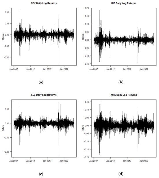
Figure 1.
Time series of the daily log returns. (a) SPY. (b) KIE. (c) XLE. (d) XME.
2.2. Climate Factor Construction
Following the approach of [34], the study constructs a climate risk factor by combining the returns of sectors with high exposure to transition risks. In their study, the climate factor was defined using the XLE and coal (KOL) indices, with weights of 30% and 70%, respectively, and then adjusted by subtracting the market return. However, since the KOL index was liquidated and therefore unavailable for a sufficiently long sample period, the study substituted the KOL index with the XME index. Importantly, XME is highly correlated with KOL (a correlation coefficient of 0.735 over the overlapping sample, where their return distributions exhibit similar central tendencies and dispersion characteristics), making it a reasonable proxy to extend the analysis to a longer horizon. To preserve comparability with the original construction, the study retained the same sectoral weights, ensuring that the new factor remains closely aligned with the original Fed specification.
Specifically, the study forms a portfolio consisting of a weight of 30% on XLE and a weight of 70% on XME, both of which represent industries heavily impacted by decarbonization policies, regulatory constraints, and changes in investor preferences. The heavier weight is placed on the XME (), consistent with the original heavy coal design, reflecting the stronger sensitivity to transition risk of coal/mining relative to the broad energy. We then subtract the return on the S&P 500 index (⌃GSPC) to isolate the excess return attributed to the risk of climate change.
The climate factor is defined as follows:
where , , and represent the returns of the Energy, Metals & Mining, and market (S&P 500) indices at time t, respectively. The constructed return of the climate factor, , captures the relative performance of the carbon-intensive sectors compared to the general market. This portfolio-based approach reflects the exposure of these sectors to transition risks, such as changes in climate regulation, carbon pricing, and changes in investor preferences toward low-emission assets. A decrease in indicates periods of increased transition pressure, while an increase reflects relaxed transition expectations.
In the insurance sector, such transition shocks can influence both the asset and liability sides of balance sheets. On the asset side, insurers’ investment portfolios may experience value losses through holdings in carbon-intensive industries. On the liability side, transition-driven macroeconomic adjustments can affect underwriting profitability and long-term solvency. Therefore, serves as a market-based proxy of insurers’ exposure to climate transition risk and is used as the climate factor in the empirical factor model.
To evaluate the robustness of this construction, several susceptibility tests are conducted. First, regressions of insurance sector returns (KIE) in SPY and the two alternative climate factors produce consistent results: the climate factor remains positive and highly significant (p < 0.001) in both cases, with negligible differences in model fit and residual variation. Finally, to assess sensitivity to the choice of sectoral weights, alternative specifications are estimated using 60/40 and 80/20 XLE-XME splits. Across all weight configurations, the estimated coefficients on the climate factor remain stable, with only marginal differences in magnitude and statistical significance. Collectively, these tests confirm that the substitution of XME for KOL, as well as moderate variations in sectoral weighting, do not materially affect the estimated results, indicating that the constructed climate factor is statistically robust.
2.3. Climate Beta Estimation
This study uses the standard factor model for stock returns and analyzes the effect of the climate factor (CF) on the insurance sector returns.
where represents the return on the insurance sector stock at time t, measures the sensitivity of the returns of the insurance stock to market risk (), and captures the sensitivity of the returns of the insurance stock to the risk of the climate factor.
To isolate the portion of insurance returns specifically attributed to climate risk, the study computes the Insurance Climate Risk (ICR) as the residual component of the regression, after accounting for the market factor.
This adjustment removes the influence of general market risk, leaving the ICR as the portion of insurance sector returns solely influenced by the CF. By isolating this component, the study aims to estimate the relationship between climate risks and the performance of the insurance sector.
2.4. Extreme Value Theory and Modeling
EVT provides robust models to capture the extreme tails of a distribution and to forecast the risk. There are two main approaches in EVT modeling: the block maxima; this models the maximum loss for each block based on the Generalized Extreme Value Distribution (GEV). However, the peak over threshold models all data that exceed a certain set high level of threshold using the Generalized Pareto Distribution (GPD).
2.4.1. Generalized Extreme Value and Block Maxima Method
Definition 1
(Generalized Extreme Value Distribution). The Generalized Extreme Value (GEV) distribution is a three-parameter family that unifies the Fréchet, Weibull, and Gumbel distributions into a single form. Its cumulative distribution function (CDF) is given by
where is the location parameter, is the scale parameter, and is the shape parameter.
2.4.2. Generalized Pareto Distribution and Peaks over Threshold
Definition 2
(Excess Distribution). Let X be a random variable with cumulative distribution function . For a given high threshold u, the excess distribution above u is defined as
where . The conditional probability can be expressed as
Theorem 1
(Pickands–Balkema–de Haan Theorem [38,39]). For a large class of underlying distributions F, the distribution of excesses over a sufficiently high threshold u converges to the Generalized Pareto Distribution (GPD), defined by
where is the shape parameter, is the scale parameter, and with α representing the tail index. Thus, for a sufficiently large u,
This result provides the theoretical foundation for the POT method. Using this approximation, the upper tail of for can be represented as
For empirical estimation, if n total observations are available and k exceeds the threshold u, can be estimated by
yielding the tail estimator.
2.5. Value at Risk and Conditional Value at Risk
Let be the loss of a portfolio over a given period. The VaR at the confidence level , denoted , is defined as
This represents the quantile function of the loss distribution at the level , ensuring that the probability of exceeding is at most . This provides a threshold beyond which extreme losses are expected to occur with a small probability.
A crucial property of this definition is that the underlying loss distribution must be continuous and invertible to ensure proper quantile determination. The limiting distribution of extreme losses satisfies these conditions in the tail-risk estimation method of extreme value theory.
Although VaR is widely used in financial risk management, it does not account for the magnitude of losses beyond the threshold. This limitation is addressed by CVaR. CVaR measures the expected loss given that the loss has exceeded VaR. CVaR at confidence level , denoted , is defined as
This formulation, introduced by [40], provides a coherent risk measure that satisfies sub-additivity and convexity properties, making it a superior alternative to VaR in many practical applications.
2.5.1. BMM VaR and CVaR
Proposition 1
(Value at Risk under the GEV distribution). Let X be a random variable following the Generalized Extreme Value (GEV) distribution with shape parameter , location parameter μ, and scale parameter σ. Then, the Value at Risk (VaR) at confidence level is given by
Proposition 2
(Conditional Value at Risk under the GEV distribution). Let X be a random variable following the Generalized Extreme Value (GEV) distribution with shape parameter , location parameter μ, and scale parameter σ. Then, the Conditional Value at Risk (CVaR) at confidence level is given by
where denotes the lower incomplete gamma function.
The expressions above provide the Block Maxima Method (BMM) estimates of VaR and CVaR, as derived from the quantile function of GEV [41]. The derivation of these results is provided in Appendix B.1 and Appendix B.2, respectively.
2.5.2. POT VaR and CVaR
Proposition 3
(Value at Risk under the GPD model). Let X denote excess losses above a threshold u, modeled by the generalized Pareto distribution (GPD) with shape parameter ξ and scale parameter ψ. Then, the Value at Risk (VaR) at confidence level is given by
Proposition 4
(Conditional Value at Risk under the GPD model). Let X denote excess losses above a threshold u, modeled by the generalized Pareto distribution (GPD) with shape parameter , scale parameter ψ, and threshold u. Then, the Conditional Value at Risk (CVaR) at confidence level is given by
Using the POT method, the GPD is fitted to the excess values, from which confidence intervals for the parameters are obtained. VaR and CVaR are then calculated as unconditional risk measures, providing a clear quantification of tail risks. The derivation of these results is provided in Appendix B.3 and Appendix B.4, respectively.
3. Results
Using the daily, weekly, and monthly returns of each index to construct and implement the climate factor, the analysis derives the climate beta estimate, which quantifies the sensitivity of the insurance index (KIE) to both market movements and climate-specific influences. Using the standard factor model, the regression analysis incorporates as the market factor and as the climate-specific factor. The study presents the climate beta estimates in Table 2.
Table 2.
Climate Beta Estimates.
The results indicate that daily returns provide the most robust information, with a statistically significant (t-value 6.202, ) and higher precision. This is attributed to daily return data that capture short-term fluctuations and market dynamics more effectively. In terms of interpretations, for each 1% increase in , increases by approximately 0.06%. While smaller than the SPY effect, this positive and statistically significant relationship suggests that climate-related factors have a negative impact on insurance returns. Although weekly returns are still significant, they show higher standard errors and lower t values for , suggesting a reduced sensitivity to short-term climate-related risks due to aggregation.
However, in the monthly returns is not statistically significant (). This means that the climate factor does not show a clear impact when using monthly data. Due to this, the study focuses on the daily and weekly return datasets, which provide clearer and more reliable insights into the connection between climate factors and the insurance sector. The positive and significant daily and weekly climate beta indicates that short-term climate shocks meaningfully affect insurance returns, highlighting insurers’ sensitivity to climate-related market dynamics. This suggests that frequent exposure monitoring is essential to manage portfolio risks and ensure capital adequacy under volatile climate conditions.
Finally, the study isolates , removes the effect of overall market movements by subtracting the SPY component using the estimated beta coefficient of the factor model. The resulting series is then used in our EVT analysis to examine the specific tail risks for the insurance sector. To focus on losses (the left tail of the return distribution), the study inverts the ICR values by setting .
The study begins our extreme value analysis with the Peaks over Threshold (POT) approach, which models all datasets that exceed a threshold u using the Generalized Pareto distribution. To determine an appropriate threshold, the study uses the empirical mean excess plot (Figure 2), which shows approximate linearity beyond the 95th percentile for both daily and weekly returns. This indicates a stable cutoff for modeling extremes. Therefore, the 95% quantile is adopted, balancing sufficient tail coverage with an adequate number of exceedances for reliable GPD estimation. Table 3 reports the number of exceedances, the estimated threshold values, and the corresponding estimates of the GPD parameters in daily, weekly, and monthly frequencies. Although the proportions of exceedance are similar, approximately 5%, the daily and weekly results are emphasized due to their larger sample sizes.
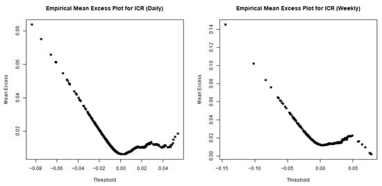
Figure 2.
Empirical mean excess function for ICR: daily log and weekly returns.
Table 3.
Parameter estimates for GPD.
Figure 3 illustrates the plot of excesses above the 95% quantile of the insurance climate risk using the daily log returns. The excess plot highlights periods of increased climate risk in the insurance sector, with a notable clustering of exceedances in 2007–2011 and 2018–2024. Between 2012 and 2017, there were fewer exceedances, suggesting a quieter period with fewer extreme events.
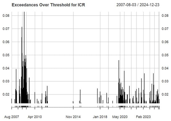
Figure 3.
Excess plot ICR for daily returns.
In addition, in Table 3, the shape parameter () is positive for the daily and weekly insurance climate risk, indicating the presence of heavy tails and a higher probability of extreme events. In contrast, the monthly insurance climate risk yields a strongly negative shape parameter, suggesting a bounded tail with limited extremity. The scale parameter (), which measures the spread of exceedances, is relatively smaller in the daily and weekly data, implying more stable and consistent exceedance magnitudes compared to the monthly insurance climate risk. These results have practical implications for the capital and solvency management of insurers. The presence of heavy tails in daily and weekly insurance climate risk indicates that extreme losses, though infrequent, can be severe. This highlights the need for higher capital hedging and more dynamic risk monitoring in climate-sensitive portfolios.
The excess distribution plot and the tail distribution plot of the ICR are shown in Figure 4. The plots show that exceedances lie close to the theoretical curves, showing that the estimated model fits the excesses.
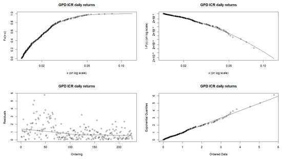
Figure 4.
GPD fit plot daily returns of ICR.
In addition to the POT approach, the study also applies the block maximum method. To fit the block maxima to the Generalized Extreme Value distribution, the study first extracts the maximum values from nonoverlapping blocks of data. These maxima are then fitted to the GEV distribution, allowing for the estimation of the model parameters and the interval estimates. The study mainly uses monthly blocks for this analysis, as using yearly blocks would contain 18 data points.
For the monthly blocks, the study performed two separate analyses using daily log returns and weekly returns. Figure 5 and Figure 6 illustrate the plot for the monthly maxima of the daily log returns and the weekly returns for the loss distribution of the ICR, respectively. The plots show closely fitting density plots for the daily and weekly returns, respectively. However, the Q-Q plot reveals that the daily returns fit better to the GEV distribution.
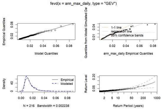
Figure 5.
Monthly Maxima of the Daily Log Returns of ICR.
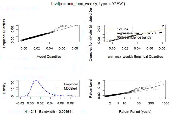
Figure 6.
Monthly Maxima of the Weekly Returns of ICR.
Table 4 gives the point and interval estimates at a 95% confidence interval for both block maxima. The point estimate for both returns indicates that the distribution of the monthly block maxima follows a Frechet distribution, indicating heavy-tailedness. This behavior demonstrates that extreme climate-related losses can increase nonlinearly, underscoring the need for insurers to improve tail risk monitoring and maintain adequate mitigation against rare but severe shocks.
Table 4.
Parameter estimates for daily and weekly returns blocked monthly.
The GEV estimates for the daily log returns blocked monthly have a lower negative log likelihood, Akaike Information Criterion, and Bayesian Information Criterion, confirming a better fit than the weekly returns blocked monthly. This means that daily log returns capture short-term changes more accurately and provide a clearer picture of extreme insurance climate-related risks.
The next study estimates the value at risk and the conditional value at risk using the parameter estimates obtained from the EVT-based GPD and GEV models. This allows us to assess the excess climate-related risk embedded in the portfolio loss distribution and to highlight its broader implications for insurance risk management. The analysis selected the appropriate return frequency for both the POT method (daily, weekly, and monthly returns) and the BMM (daily log returns blocked monthly and weekly log returns blocked monthly), as they offer different perspectives on extreme losses.
Table 5 reports the estimated VaR and CVaR in the different return frequencies and methods, providing a comprehensive view of how extreme losses vary depending on the modeling approach.
Table 5.
Value at Risk and Conditional Value at Risk estimates.
From the above table, the POT daily estimates indicate that the insurance climate risk portfolio is not expected to lose more than 1.327% in a given day. However, if this threshold is breached, the expected loss increases to approximately 2.284%, reflecting the severity of extreme climate-driven shocks. In contrast, the Block Maxima method applied to daily returns blocked monthly produces higher tail risk estimates, with a VaR of 3.642% and a CVaR of 5.681%.
A clear pattern emerges across the insurance climate risk frequencies, as both VaR and CVaR increase substantially from the daily to monthly frequencies. Under the POT method, the daily returns yield the lowest tail risk estimates, while the monthly returns show the largest. The increase across frequencies highlights that climate risk exposure in insurance portfolios becomes more pronounced when shocks are considered over extended periods.
The BMM results also point to an increased climate-related risk compared to daily POT estimates, particularly for weekly returns blocked monthly. The study shows the sensitivity of extreme value estimates to different methodological choices. For insurers, both perspectives are important, since POT emphasizes recurring exceedances, while BMM isolates the largest, potentially catastrophic events. In general, Table 5 highlights that insurance climate risk is characterized by heavy-tailed loss distributions, with both POT and BMM confirming substantial exposure to extreme events. These findings highlight the need for insurers to better account for rare but severe climate shocks when assessing portfolio resilience and designing long-term risk management strategies.
4. Conclusions
This study presents an integrated framework for assessing the climate-related tail risk exposure of the US insurance sector by combining factor modeling with Extreme Value Theory. Using a climate factor constructed from transition-sensitive sectors (energy and metals/mining), the study estimated the exposure of the SPDR S&P Insurance ETF (KIE) to climate-specific risks. By controlling for general market movements through the use of the S&P 500 index, the analysis isolated the insurance climate risk component and applied EVT to model the behavior of extreme negative returns.
The results of the factor model indicate that climate risk has a significant influence on insurance sector returns, particularly at the daily and weekly frequencies. Recent research supports these findings. For example, ref. [42] shows that climate risk shocks are reflected in portfolio returns and can be hedged using factor-based methods, while ref. [43] shows that the dependencies between transition and physical climate risks significantly impact insurance asset-liability exposures. This suggests that short-term market dynamics are highly sensitive to movements related to the transition. The EVT analysis, employing both the Peaks Over Threshold method with the Generalized Pareto distribution and the Block Maxima method with the Generalized Extreme Value distribution, consistently revealed heavy-tailed characteristics in the insurance climate loss distribution. Across both methods, VaR and CVaR estimates increased with weekly and monthly data, indicating that tail risks become more pronounced over longer horizons.
The primary contribution of this study lies in the approach to isolating climate-specific financial risk and examining its tail behavior. Compared to existing studies on the estimation of financial climate risk, which mainly focus on general market indices or aggregate sectoral exposure [44,45], our methodology explicitly isolates insurance climate risk and applies EVT to tail events. By focusing on insurance climate risk, distinct from general market movements, and applying both the POT and BMM frameworks, the analysis provides a clearer assessment of the potential losses insurers may face from climate-related shocks. This methodology improves our understanding of how climate risk translates into extreme financial outcomes and offers a more targeted measure of vulnerability for the insurance sector.
From a practical perspective, the findings highlight the importance of incorporating climate-sensitive factors into financial risk management frameworks. For regulators and insurers, recognizing the heavy-tailed nature of climate-induced risks makes it crucial to account for these shocks in portfolio allocation, pricing, and reserve strategies. Furthermore, the results demonstrate that the impact of climate risks is not uniform across time horizons, implying that risk management strategies must differentiate between short-term volatility and long-term tail exposures.
Finally, this work opens several avenues for future research. Extending the factor construction to include physical climate risks (e.g., hurricane damage, wildfire exposures) alongside transition risks could yield a more comprehensive measure of insurance vulnerability. In addition, applying the framework to a broader set of financial institution data would allow comparative insights into climate risk exposures across markets. These extensions also address current limitations, as the present analysis focuses primarily on transition risks and the US insurance sector, and assumes that historical tail behavior reflects future extremes. Integrating scenario analysis and forward-looking climate policy pathways could further enhance the predictive capacity of the EVT-based approach.
In summary, this study demonstrates that climate-related risks are material, quantifiable, and concentrated in the tails of the return distribution of the insurance sector. By providing an EVT-based methodology tailored to climate risk exposure, the study contributes to both the academic literature on financial econometrics and the ongoing policy debate on climate-related financial stability.
Funding
This research received no external funding.
Data Availability Statement
The data presented in this study are openly available in Yahoo Finance at https://finance.yahoo.com/, accessed on 1 September 2025. All analysis was conducted in RStudio (2024.09.0+375), and the processed data outputs are available from the author upon request.
Acknowledgments
The author would like to thank Qiji Jim Zhu for suggesting the research direction and methodological approach for this paper. This work is based on my master’s thesis, completed under his supervision. I would also like to acknowledge our productive group discussions with Hala Alkhalid, which contributed to this work.
Conflicts of Interest
The author declare no conflicts of interest.
Abbreviations
The following abbreviations are used in this manuscript:
| EVT | Extreme Value Theorem |
| VaR | Value at Risk |
| CVaR | Conditional Value at Risk |
| GPD | Generalized Pareto Distribution |
| GEV | Generalized Extreme Value |
| POT | Peak over Threshold |
| BMM | Block Maxima Method |
| CF | Climate Factor |
| ICR | Insurance Climate Risk |
Appendix A
Appendix A.1
Table A1.
Descriptive statistics for the weekly and monthly returns of SPY, KIE, XLE, and XME.
Table A1.
Descriptive statistics for the weekly and monthly returns of SPY, KIE, XLE, and XME.
| Returns | Index | Mean | Std | Skewness | Kurtosis |
|---|---|---|---|---|---|
| Weekly | SPY | 0.00184 | 0.02520 | −0.60950 | 6.65853 |
| KIE | 0.00180 | 0.03568 | −0.34148 | 13.28531 | |
| XLE | 0.00122 | 0.03949 | −0.57014 | 5.63482 | |
| XME | 0.00153 | 0.05192 | −0.06874 | 3.08200 | |
| Monthly | SPY | 0.00766 | 0.04519 | −0.58545 | 0.96502 |
| KIE | 0.00713 | 0.06351 | −0.78341 | 4.11487 | |
| XLE | 0.00493 | 0.07795 | −0.01933 | 3.48727 | |
| XME | 0.00601 | 0.10139 | −0.18466 | 0.67105 |
Appendix B
Appendix B.1
Proof of Proposition 1.
Let X be a loss variable and assume that the block maxima of X follow a Generalized Extreme Value (GEV) distribution with location parameter , scale parameter , and shape parameter . The cumulative distribution function is
By definition, the VaR at confidence level is the -quantile of :
Substituting the GEV CDF,
Taking the natural logarithm and rearranging,
Solving for , we obtain the VaR under the BMM:
This completes the derivation. □
Appendix B.2
Proof of Proposition 2.
We begin with the quantile-based definition of Conditional Value-at-Risk (CVaR) for a continuous distribution:
The quantile function for the Generalized Pareto Distribution is given by
Substituting the quantile function into the CVaR formula yields
Let . We solve this integral using the substitution:
The limits change as follows: when , ; when , . Applying the substitution
The resulting integral is the lower incomplete Gamma function:
where is the lower incomplete Gamma function. Therefore, . Substituting back into the expression for CVaR,
This completes the derivation. □
Appendix B.3
Proof of Proposition 3.
Let X be a loss variable, u a high threshold, and let exceedances follow a GPD with shape and scale :
Let k of the observations n exceed u, so . For ,
The -quantile satisfies , yielding
Solving for gives the POT VaR:
This completes the derivation. □
Appendix B.4
Proof of Proposition 4.
Let X be a loss variable and the POT VaR at confidence level , with exceedances over threshold u following a GPD with shape and scale . By definition, the Conditional Value at Risk is the tail expectation expressed via the quantile function:
Substituting the POT VaR formula
we integrate over . Evaluating this integral gives
This completes the derivation. □
References
- Campiglio, E.; Daumas, L.; Monnin, P.; von Jagow, A. Climate-related risks in financial assets. J. Econ. Surv. 2023, 37, 950–992. [Google Scholar] [CrossRef]
- Hjort, I.A. Potential Climate Risks in Financial Markets: A Literature Overview; Memorandum; Institute of Pacific Relations, American Council: New York, NY, USA, 2016; Available online: https://api.semanticscholar.org/CorpusID:55356987 (accessed on 7 August 2025).
- Avramov, D.; Cheng, S.; Lioui, A.; Tarelli, A. Sustainable investing with ESG rating uncertainty. J. Financ. Econ. 2022, 145, 642–664. [Google Scholar] [CrossRef]
- Thistlethwaite, J.; Wood, M.O. Insurance and Climate Change Risk Management: Rescaling to Look Beyond the Horizon. Br. J. Manag. 2018, 29, 279–298. [Google Scholar] [CrossRef]
- Schuh, F.; Jaeckle, T. Impact of hurricanes on US insurance stocks. Risk Manag. Insur. Rev. 2023, 26, 5–34. [Google Scholar] [CrossRef]
- Bressan, G.; Đuranović, A.; Monasterolo, I.; Battiston, S. Asset-level assessment of climate physical risk matters for adaptation finance. Nat. Commun. 2024, 15, 5371. [Google Scholar] [CrossRef] [PubMed]
- Acharya, V.V.; Johnson, T.; Sundaresan, S.; Tomunen, T. Is Physical Climate Risk Priced? Evidence from Regional Variation in Exposure to Heat Stress; NBER Working Paper, No. w30445; National Bureau of Economic Research: Cambridge, MA, USA, 2022. [Google Scholar] [CrossRef]
- Weber, O.; Dordi, T.; Oyegunle, A. Stranded Assets and the Transition to Low-Carbon Economy. In Sustainability and Financial Risks; Palgrave Studies in Impact Finance; Migliorelli, M., Dessertine, P., Eds.; Palgrave Macmillan: Cham, Switzerland, 2020. [Google Scholar] [CrossRef]
- Bolton, P.; Kacperczyk, M. Do investors care about carbon risk? J. Financ. Econ. 2021, 142, 517–549. [Google Scholar] [CrossRef]
- Bolton, P.; Kacperczyk, M. Global pricing of carbon-transition risk. J. Financ. 2023, 78, 3677–3754. [Google Scholar] [CrossRef]
- Carbone, S.; Giuzio, M.; Kapadia, S.; Krämer, J.S.; Nyholm, K.; Vozian, K. The Low-Carbon Transition, Climate Commitments and Firm Credit Risk; Sveriges Riksbank Working Paper Series, No. 409; Sveriges Riksbank: Stockholm, Sweden, 2022. Available online: https://hdl.handle.net/10419/251307 (accessed on 7 August 2025).
- Reboredo, J.C.; Ugolini, A. Climate transition risk, profitability and stock prices. Int. Rev. Financ. Anal. 2022, 83, 102271. [Google Scholar] [CrossRef]
- Engle, R.F.; Giglio, S.; Kelly, B.; Lee, H.; Stroebel, J. Hedging Climate Change News. Rev. Financ. Stud. 2020, 33, 1184–1216. [Google Scholar] [CrossRef]
- Krueger, P.; Sautner, Z.; Starks, L.T. The Importance of Climate Risks for Institutional Investors. Rev. Financ. Stud. 2020, 33, 1067–1111. [Google Scholar] [CrossRef]
- Bank for International Settlements. The Green Swan: Central Banking and Financial Stability in the Age of Climate Change; BIS Publications: New Delhi, India, 2020; Available online: https://www.bis.org/publ/othp31.htm (accessed on 7 August 2025).
- International Monetary Fund. Chapter 5: Climate Change: Physical Risk and Equity Prices; Global Financial Stability Report, No. 2020/001; International Monetary Fund: Washington, DC, USA, 2020; Available online: https://www.imf.org/en/Publications/GFSR/Issues/2020/04/14/global-financial-stability-report-april-2020#Chapter5 (accessed on 7 August 2025).
- Network for Greening the Financial System (NGFS). Enhancing Market Transparency in Green and Transition Finance. NGFS Technical Document. 2022 April. Available online: https://www.ngfs.net/sites/default/files/medias/documents/enhancing_market_transparency_in_green_and_transition_finance.pdf (accessed on 7 August 2025).
- Laliotis, M.D.; Lamichhane, S. Delays in Climate Transition Can Increase Financial Tail Risks: A Global Lesson from a Study in Mexico; International Monetary Fund: Washington, DC, USA, 2023. [Google Scholar]
- Morgan, J.P. RiskMetrics—Technical Document; J.P. Morgan/Reuters: New York, NY, USA, 1996. [Google Scholar]
- Artzner, P. Thinking coherently. Risk 1997, 10, 68–71. [Google Scholar]
- Artzner, P.; Delbaen, F.; Eber, J.M.; Heath, D. Coherent measures of risk. Math. Financ. 1999, 9, 203–228. [Google Scholar] [CrossRef]
- McNeil, A.J.; Frey, R. Estimation of tail-related risk measures for heteroscedastic financial time series: An extreme value approach. J. Empir. Financ. 2000, 7, 271–300. [Google Scholar] [CrossRef]
- Li, L. A Comparative Study of GARCH and EVT Model in Modeling Value-at-Risk. 2017. Available online: https://mpra.ub.uni-muenchen.de/85645/ (accessed on 7 August 2025).
- Singh, A.K.; Allen, D.E.; Powell, R.J. Value at Risk Estimation Using Extreme Value Theory. 2011. Available online: http://ro.ecu.edu.au/ecuworks2011/721/ (accessed on 7 August 2025).
- Embrechts, P.; Resnick, S.I.; Samorodnitsky, G. Extreme value theory as a risk management tool. N. Am. Actuar. J. 1999, 3, 30–41. [Google Scholar] [CrossRef]
- Chaudhry, S.M.; Chen, X.H.; Ahmed, R.; Nasir, M.A. Risk modelling of ESG (environmental, social, and governance), healthcare, and financial sectors. Risk Anal. 2025, 45, 477–495. [Google Scholar] [CrossRef] [PubMed]
- Soltane, H.B.; Karaa, A.; Bellalah, M. Conditional VaR using GARCH-EVT approach: Forecasting volatility in Tunisian financial market. J. Comput. Model. 2012, 2, 95–115. [Google Scholar]
- Echaust, K.; Just, M. Value at risk estimation using the GARCH-EVT approach with optimal tail selection. Mathematics 2020, 8, 114. [Google Scholar] [CrossRef]
- Weber, O. Climate stress testing in the financial industry. Curr. Opin. Environ. Sustain. 2024, 66, 101401. [Google Scholar] [CrossRef]
- Alexander, C.; Sheedy, E. Developing a stress testing framework based on market risk models. J. Bank. Financ. 2008, 32, 2220–2236. [Google Scholar] [CrossRef]
- Battiston, S.; Dafermos, Y.; Monasterolo, I. Climate risks and financial stability. J. Financ. Stab. 2021, 54, 100867. [Google Scholar] [CrossRef]
- Acharya, V.V.; Berner, R.; Engle, R.; Jung, H.; Stroebel, J.; Zeng, X.; Zhao, Y. Climate stress testing. Annu. Rev. Financ. Econ. 2023, 15, 291–326. [Google Scholar] [CrossRef]
- Dietz, S.; Bowen, A.; Dixon, C.; Gradwell, P. ‘Climate value at risk’ of global financial assets. Nat. Clim. Change 2016, 6, 676–679. [Google Scholar] [CrossRef]
- Jung, H.; Engle, R.F.; Berner, R.B. Climate Stress Testing. Staff Reports, No. 977. 2021. Available online: https://hdl.handle.net/10419/247900 (accessed on 7 August 2025).
- Vansteenberghe, E. Insurance Supervision Under Climate Change: A Pioneers Detection Method. 2023. Available online: https://shs.hal.science/halshs-04350178v1/file/wp_202343_.pdf (accessed on 7 August 2025).
- Olaniyan, O. Estimating Climate Risk in Financial Markets. Master’s Thesis, Department of Mathematics, Western Michigan University, Kalamazoo, MI, USA, 2025. Available online: https://scholarworks.wmich.edu/masters_theses/5462 (accessed on 7 August 2025).
- Litterman, R. Selling Stranded Assets: Profit, Protection, and Prosperity. 2023. Available online: https://www.intentionalendowments.org/selling_stranded_assets_profit_protection_and_prosperity (accessed on 7 August 2025).
- Pickands, J., III. Statistical inference using extreme order statistics. Ann. Stat. 1975, 119–131. [Google Scholar]
- Balkema, A.A.; de Haan, L. Residual life time at great age. Ann. Probab. 1974, 792–804. [Google Scholar] [CrossRef]
- Rockafellar, R.T.; Uryasev, S. Optimization of conditional value-at-risk. J. Risk 2000, 2, 21–42. [Google Scholar] [CrossRef]
- Khokhlov, V. Conditional Value-at-Risk for Uncommon Distributions. 21 June 2018. Available online: https://ssrn.com/abstract=3200629 (accessed on 7 September 2025).
- Alekseev, G.; Giglio, S.; Maingi, Q.; Selgrad, J.; Stroebel, J. A Quantity-Based Approach to Constructing Climate Risk Hedge Portfolios; NBER Working Paper, No. 30703; National Bureau of Economic Research: Cambridge, MA, USA, 2022. [Google Scholar] [CrossRef]
- Gatzert, N.; Özdil, O. The impact of dependencies between climate risks on the asset and liability side of non-life insurers. Eur. Actuar. J. 2024, 14, 1–19. [Google Scholar] [CrossRef]
- Riaman, R.; Supian, S.; Sukono, S.; Mamat, M.; Bon, A. Estimated Value at Risk in Stock Investments in an Insurance Company Using the Extreme Value Theory Method. In Proceedings of the 2nd African International Conference on Industrial Engineering and Operations Management, Harare, Zimbabwe, 7–10 December 2020; Available online: https://index.ieomsociety.org/index.cfm/article/view/ID/6947 (accessed on 14 October 2025).
- Maelowati, I.D.; Mayaningtyas, C.A. Risk Prediction and Estimation of Corporate Product Claim Reserve Funds in Insurance Companies Using the Extreme Value Theory. Int. J. Quant. Res. Model. 2024. Available online: https://api.semanticscholar.org/CorpusID:275352088 (accessed on 14 October 2025). [CrossRef]


Disclaimer/Publisher’s Note: The statements, opinions and data contained in all publications are solely those of the individual author(s) and contributor(s) and not of MDPI and/or the editor(s). MDPI and/or the editor(s) disclaim responsibility for any injury to people or property resulting from any ideas, methods, instructions or products referred to in the content. |
© 2025 by the author. Licensee MDPI, Basel, Switzerland. This article is an open access article distributed under the terms and conditions of the Creative Commons Attribution (CC BY) license (https://creativecommons.org/licenses/by/4.0/).