A Space–Time Collocation Method Using the Method of Particular Solutions with Polynomial Basis Functions for Solving the Fisher–KPP Equation

Abstract

The method of particular solutions (MPS) has been widely applied for solving various types of partial differential equations. In this paper, the space–time collocation technique is implemented using MPS with polynomial basis functions (MPS-PBF) to solve the nonlinear Fisher–KPP (Kolmogorov–Petrovsky–Piskunov) equation in both one and two dimensions. The Picard iteration method is used to deal with the nonlinearity of the problem. Four numerical examples are provided, and their results are compared with established methods to demonstrate the effectiveness of the proposed scheme.

1. Introduction

The Fisher equation was first introduced by Roland A. Fisher in 1937 in the context of population dynamics [1] and later independently studied by Andrey Kolmogorov, Ilya Petrovsky, and Nikolai Piskunov in the same year [2]. The Fisher–KPP equation is a nonlinear time-dependent partial differential equation (PDE) that models the spread of an advantageous gene, species, or other phenomena in a spatial domain over time. This equation is a special case of the reaction–diffusion equation and one of the important nonlinear equations in the field of science, which describes how a population (or any diffusive quantity) grows and spreads in space [3]. Numerous numerical methods have been used to solve the Fisher–KPP equation in the literature. The finite difference method is one of the most popular mesh-based approaches for solving the Fisher–KPP equation numerically [4,5]. Vimal et.al. used the backward differentiation formula for solving the nonlinear Fisher equation [6]. Similarly, many researchers have also employed the finite element method and the Galerkin method while solving the Fisher–KPP equation or the reaction–diffusion equation in general [7,8].

Meshless methods using radial basis functions are a class of numerical techniques that can be used to solve various types of linear and nonlinear PDEs without relying on a traditional mesh structure, which are very useful when the domain is irregular or where mesh generation is complex or computationally expensive [9,10,11,12]. Zhang et al. used the RBF-FD method for the numerical study of Fisher’s equation [13]. Recently, the space–time collocation method has emerged as a novel meshless method in the literature for solving various types of PDEs. Hamaidi et al. introduced the space–time localized radial basis function collocation method for solving parabolic and hyperbolic equations [14]. Cao et al. employed the space–time polynomial particular solutions method for solving time-dependent problems [15]. Our motivation stems from the need for a more efficient and accurate solution to complex, nonlinear, time-dependent problems such as the Fisher–KPP equation in both one-dimensional (1D) and two-dimensional (2D) settings. In this work, we examine the effectiveness of the space–time collocation method using the method of particular solutions with polynomial basis functions (MPS-PBF) for solving the Fisher–KPP equation.

The structure of the paper is as follows: Section 2 demonstrates the comprehensive solution methodology of the space-time collocation method using the polynomial basis functions. In Section 3, we provide the numerical results, numerical simulations, and their analysis in detail. Finally, the conclusion and the outlines for the future research directions are furnished in Section 4.

2. Solution Methodology

2.1. Space-Time Collocation Technique

Consider the equation

$${\displaystyle \frac{\partial u(\mathbf{x},t)}{\partial t}}=D\Delta u(\mathbf{x},t)+\alpha u(\mathbf{x},t)(1-u^{\beta }(\mathbf{x},t))+f(\mathbf{x},t),\mathbf{x}\in \mathsf{\Omega },0<t\le T,$$

(1)

with an initial condition

$$u(\mathbf{x},0)=u_0\left(\mathbf{x}\right),\mathbf{x}\in \mathsf{\Omega },$$

(2)

and the Dirichlet boundary condition

$$Bu(\mathbf{x},t)=g(\mathbf{x},t),\mathbf{x}\in \partial \mathsf{\Omega },0<t\le T.$$

(3)

Here, D is the diffusion coefficient that tells us the rate at which the quantity $u(\mathbf{x},t)$ spreads spatially over time, $\alpha$ and $\beta$ are the reaction parameters and $f(\mathbf{x},t)$ is the forcing term. Traditionally, time-dependent problems are treated by discretizing the temporal domain using time-stepping schemes, such as Euler’s method, and subsequently applying a collocation method in the spatial domain at each step. In contrast, the space–time collocation technique regards the temporal variable as an additional spatial dimension, thereby transforming a d-dimensional time-dependent problem into an $(d+1)$-dimensional problem posed entirely in the spatial domain. The corresponding extended computational domains are depicted in Figure 1. Under this reformulation, the problem takes the following form:

$${\displaystyle \frac{\partial u(\mathbf{x},t)}{\partial t}}=D\Delta u(\mathbf{x},t)+\alpha u(\mathbf{x},t)(1-u^{\beta }(\mathbf{x},t))+f(\mathbf{x},t),(\mathbf{x},t)\in \mathsf{\Omega }\times (0,T),$$

(4)

with boundary conditions

$$u(\mathbf{x},0)=u_0\left(\mathbf{x}\right),(\mathbf{x},0)\in \mathsf{\Omega }\times \left\{t=0\right\}=\partial {\mathsf{\Omega }}_1,$$

(5)

$$Bu(\mathbf{x},t)=g(\mathbf{x},t),(\mathbf{x},t)\in \partial \mathsf{\Omega }\times (0,T]=\partial {\mathsf{\Omega }}_2,$$

(6)

$${\displaystyle \frac{\partial u(\mathbf{x},T)}{\partial t}}=D\Delta u(\mathbf{x},T)+\alpha u(\mathbf{x},T)(1-u^{\beta }(\mathbf{x},T))+f(\mathbf{x},T),(\mathbf{x},T)\in \mathsf{\Omega }\times \left\{t=T\right\}=\partial {\mathsf{\Omega }}_3,$$

(7)

where $\mathsf{\Omega }$ is the interior of the spatial domain in the $d-$dimension, and $\partial {\mathsf{\Omega }}_1$, $\partial {\mathsf{\Omega }}_2$, $\partial {\mathsf{\Omega }}_3$ are the boundaries of the extended space–time domain in $d+1$ dimensions as depicted in Figure 1b. We rewrite Equations (4)–(7) as follows:

$$D\Delta u(\mathbf{x},t)-{\displaystyle \frac{\partial u(\mathbf{x},t)}{\partial t}}+\alpha u(\mathbf{x},t)=\alpha u{(\mathbf{x},t)}^{\beta +1}+f(\mathbf{x},t),(\mathbf{x},t)\in \mathsf{\Omega }\times (0,T),$$

(8)

with boundary conditions

$$u(\mathbf{x},0)=u_0\left(\mathbf{x}\right),(\mathbf{x},0)\in \partial {\mathsf{\Omega }}_1,$$

(9)

$$Bu(\mathbf{x},t)=g(\mathbf{x},t),(\mathbf{x},t)\in \partial {\mathsf{\Omega }}_2,$$

(10)

$$D\Delta u(\mathbf{x},T)-{\displaystyle \frac{\partial u(\mathbf{x},T)}{\partial t}}+\alpha u(\mathbf{x},T)=\alpha u{(\mathbf{x},T)}^{\beta +1}+f(\mathbf{x},T),(\mathbf{x},T)\in \partial {\mathsf{\Omega }}_3.$$

(11)

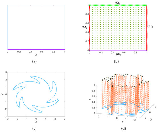
Figure 1. Examples of computational domains in space–time collocation technique. (a) Domain in 1D. (b) Extended 2D domain in space–time scheme. (c) Domain in 2D. (d) Extended 3D domain in space–time scheme.

2.2. Polynomial Basis Functions

Let

$$p_l(x,t)=x^{i-j}{t}^j,0\le i\le r,0\le j\le i,1\le l\le \gamma ,(\mathbf{x},t)\in {\mathbb{R}}^2$$

and

$$p_l(x,y,t)=x^{i-j-k}{y}^j{t}^k,0\le i\le r,0\le j\le i,0\le k\le i-j,1\le l\le \gamma ,(\mathbf{x},t)\in {\mathbb{R}}^3.$$

These sequences of monomials form a basis for the polynomials of degree less than or equal to r in 2D and 3D, respectively. Here, $\gamma =(r+1)(r+2)/2$ and $\gamma =(r+1)(r+2)(r+3)/6$ give the dimension of the polynomial basis functions space in 2D and 3D, respectively. The MPS-PBF employs the particular solutions of the polynomial basis functions for the given differential operator to approximate the solution of the partial differential equation. The closed-form particular solutions of polynomial basis functions for general linear second-order partial differential operators with constant coefficients have been derived by Dangal et al. [10].

2.3. Numerical Discretization of Fisher–KPP Equation Using MPS-PBF

Consider the Fisher–KPP Equations (1)–(3) defined on the interior of the domain $\mathsf{\Omega }$ with boundary $\partial \mathsf{\Omega }$. Following the space-time collocation scheme, the equation is transformed into the form given by Equations (8)–(11). The solution $u(\mathbf{x},t)$ to the transformed Equations (8)–(11) in the $(d+1)$-dimensional space is then approximated as $\widehat{u}(\mathbf{x},t)$ using the MPS-PBF method as follows:

$$\widehat{u}(\mathbf{x},t)=\sum _{k=1}^{\gamma }{\omega }_k{P}_k(\mathbf{x},t),$$

(12)

where

$$\left(D\Delta -{\displaystyle \frac{\partial }{\partial t}}+\alpha I\right)P_k(\mathbf{x},t)=p_k(\mathbf{x},t),k=1,2,3,...,\gamma .$$

We employ the Picard iteration algorithm to handle the nonlinear term on the right-hand side of Equations (8)–(11). Together with the Equation (12), this leads, at each iteration step n, to the following linearized system of equations:

$$\begin{array}{c}\hfill \sum _{k=1}^{\gamma }{\omega }_k^n{p}_k(\mathbf{x},t)=\alpha {\left({\widehat{u}}^{n-1}\right)}^{\beta +1}+f(\mathbf{x},t),(\mathbf{x},t)\in \mathsf{\Omega }\times (0,T),\end{array}$$

(13)

with boundary conditions

$$\sum _{l=1}^{\gamma }{\omega }_k^n{P}_k(\mathbf{x},t)=u_0\left(\mathbf{x}\right),(\mathbf{x},0)\in \partial {\mathsf{\Omega }}_1,$$

(14)

$$\sum _{l=1}^{\gamma }{\omega }_k^n{P}_k(\mathbf{x},t)=g(\mathbf{x},t),(\mathbf{x},t)\in \partial {\mathsf{\Omega }}_2,$$

(15)

$$\begin{array}{c}\hfill \sum _{k=1}^{\gamma }{\omega }_k^n{p}_k(\mathbf{x},t)=\alpha {\left({\widehat{u}}^{n-1}\right)}^{\beta +1}+f(\mathbf{x},T),(\mathbf{x},T)\in \partial {\mathsf{\Omega }}_3.\end{array}$$

(16)

In the Picard iteration, starting from an initial guess, the right-hand side term ${\widehat{u}}^{n-1}$ is computed using previously obtained coefficients $w_k^{n-1}$. Once the system is set up, the linearized Equations (13)–(16) are solved to determine the weighting coefficients ${\omega }_k^n$, from which the approximate solution is then evaluated using Equation (12).

2.4. Multiple Scale Technique

In the numerical experiments, higher-order polynomial basis functions are employed to achieve high accuracy. However, increasing the polynomial order leads to a highly ill-conditioned matrix in the MPS-PBF method. To address this issue, we adopt the multiple-scale technique [16], which significantly improves the condition number of the resulting matrix, thereby enhancing both stability and accuracy. This technique involves normalizing each column of the matrix, followed by solving a new system of equations to recover the unknown coefficients ${\omega }_k^n$.

3. Numerical Results

In this section, we present four numerical examples to demonstrate the effectiveness of our proposed numerical scheme. In all experiments presented in this article, the initial guess and stopping tolerance for the Picard iteration are set to zero and $1\times {10}^{-9}$, respectively. Unless stated otherwise, the order of the polynomial basis functions is 13.

The numerical accuracy is measured by root mean square error (RMSE), and $l_{\infty }$ error defined as

$$\begin{array}{c}\hfill \mathrm{RMSE}=\sqrt{{\displaystyle \frac{1}{\mathcal{N}}}\sum _{k=1}^{\mathcal{N}}{\left[u\left({\xi }_k\right)-\widehat{u}\left({\xi }_k\right)\right]}^2}\end{array}$$

and

$$\begin{array}{c}\hfill l_{\infty }=\underset{k}{max}|u\left({\xi }_k\right)-\widehat{u}\left({\xi }_k\right)|,\end{array}$$

where $\mathcal{N}$ is the total number of test nodes ${\xi }_k.$

Example 1. 

In this example, we consider the Fisher–KPP Equations (1)–(3) on the interval $[0,1]$ with parameter $D=\beta =1$. For this numerical experiment, $u_0$, $f,$ and g are derived from the following analytical solution [6]:

$$\begin{array}{c}\hfill u(x,t)={\displaystyle \frac{1}{{\left(1+e^{\left(\sqrt{\frac{\alpha }{6}}x-\frac{5}{6}\alpha t\right)}\right)}^2}},\mathbf{x}\in \mathsf{\Omega },0<t\le T.\end{array}$$

In the first experiment, the spatial domain $[0,1]$ is discretized with mesh size $\delta x=0.1$, time step $\delta t=0.001$, and parameter $\alpha =1$. The extended 2D domain in the space–time scheme is depicted in Figure 1b. Figure 2 displays the absolute error profiles over the domain at various time instances. The results indicate that the proposed method produces highly accurate solutions across different time instances.

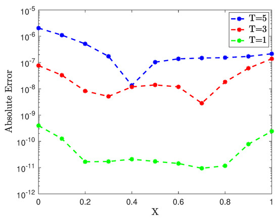
Figure 2. Example 1: Absolute error at different time instances on $[0,1]$.

However, we observe that the method performs well at early time instances, while the error gradually increases as time progresses, as shown in Figure 3.

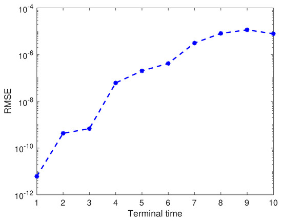
Figure 3. Example 1: RMSE at different time instances on $[1,10]$.

Next, we apply our scheme to compute approximate solutions over a larger spatial domain $[-15,15]$ with a terminal time $T=0.5$, using a mesh size of $\delta x=0.1$ and a time step of $\delta t=0.09$. As the domain size increases, we observe that higher-order polynomial basis functions are required to maintain accuracy. This highlights the important role of the multi-scale technique in achieving stable and accurate results. To investigate this effect, we solve the problem using different orders of polynomial basis functions, both with and without the multi-scale technique. Figure 4 clearly illustrates the advantage of incorporating the multi-scale technique, demonstrating its effectiveness in enhancing stability and accuracy.

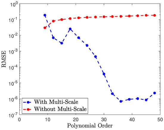
Figure 4. Example 1: Profile of RMSE versus polynomial order.

Figure 5 presents both the approximate and exact solutions for $\alpha =1$ at various time instances. The mesh size of the spatial domain and the temporal step size are set to $\delta x=0.1$ and $\delta t=0.06$, respectively. The number of interior and boundary nodes in the extended computation domain will then be $n_i=1500$ and $n_b=612$, respectively. The polynomial basis functions of order 30 are employed to obtain the results on the spatial domain $[-15,15]$. As shown in Figure 5, the approximate solution closely matches the exact solution across all time instances, demonstrating the accuracy and effectiveness of our scheme in solving the Fisher–KPP equation.

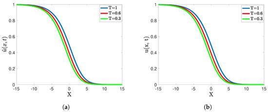
Figure 5. Example 1: (a) Profile of approximate solutions at three time instances. (b) Profile of exact solution at three time instances.

As a final experiment for this example, we compare our results at various spatial locations with those obtained using the third-order backward difference formula from [6], for the case $\alpha =6$ and terminal time $T=0.1.$ The computations are performed on the domain $[0,1]$ with a time step of $\delta t=0.000005$ and mesh size $\delta x=0.1$. As shown in Table 1, our method yields significantly more accurate results compared to the backward difference formula. Additionally, our approach can be readily extended to solve Fisher–KPP equations defined on higher-dimensional irregular domains as compared to the backward difference formula.

Table 1. Example 1: Comparison of absolute error from BDF3 [6] and MPS-PBF methods.

	BDF3	MPS-PBF
$\mathbf{x}$	Absolute Error	Absolute Error
0.1	6.754 × ${10}^{-6}$	7.173 × ${10}^{-10}$
0.2	9.522 × ${10}^{-6}$	2.344 × ${10}^{-10}$
0.3	1.175 × ${10}^{-5}$	2.152 × ${10}^{-10}$
0.4	1.332 × ${10}^{-5}$	1.739 × ${10}^{-10}$
0.5	1.415 × ${10}^{-5}$	1.388 × ${10}^{-10}$
0.6	1.415 × ${10}^{-5}$	1.213 × ${10}^{-10}$
0.7	1.319 × ${10}^{-5}$	8.314 × ${10}^{-11}$
0.8	1.106 × ${10}^{-5}$	2.045 × ${10}^{-11}$
0.9	7.500 × ${10}^{-6}$	2.531 × ${10}^{-10}$

Example 2. 

In this example, we solve the Fisher–KPP Equations (1)–(3) with the parameter $D=\alpha =1,$ and investigate the effect of varying β on the solution behavior. Here, $u_0, f,$ and g are obtained from the following analytical solution [13]:

$$\begin{array}{c}\hfill u(x,t)={\left\{{\displaystyle \frac{1}{2}}tanh\left(-{\displaystyle \frac{\beta }{2\sqrt{2\beta +4}}}\left(x-{\displaystyle \frac{\beta +4}{\sqrt{2\beta +4}}}t\right)\right)+{\displaystyle \frac{1}{2}}\right\}}^{{\displaystyle \frac{2}{\beta }}},x\in \mathsf{\Omega },0<t\le T.\end{array}$$

First, we solve this problem for $\beta =1$ and investigate the effect of varying the time step at three different time instances as shown in Figure 6. The mesh size of the spatial domain $[0,1]$ is set at $\delta x=0.1$ for this experiment. We observe that our method remains stable and provides highly accurate results, showing low sensitivity to changes in the time step.

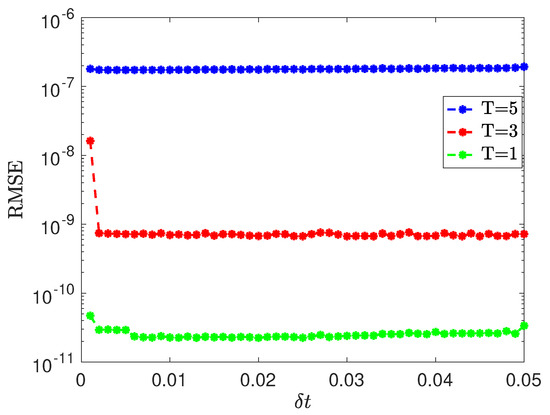
Figure 6. Example 2: Profile of RMSE versus time step.

Next, we solve this example at various time instances with $\delta t=0.011$, as reported in Table 2. The results demonstrate the high accuracy of our scheme. Furthermore, we observe better accuracy for smaller time instances, which is consistent with the findings from our previous example.

Table 2. Example 2: Error estimates at different time instances.

T	$\mathit{RMSE}$	${\mathit{l}}_{\mathit{\infty }}$
1	2.259 × ${10}^{-11}$	1.265 × ${10}^{-10}$
3	6.835 × ${10}^{-10}$	5.329 × ${10}^{-9}$
5	1.729 × ${10}^{-7}$	1.962 × ${10}^{-6}$
7	2.669 × ${10}^{-6}$	3.676 × ${10}^{-5}$
10	7.168 × ${10}^{-6}$	3.120 × ${10}^{-5}$

As a further experiment, we solve this problem for several values of $\beta$. The corresponding RMSE with respect to the time step at $T=1$ for three representative values of $\beta$ is depicted in Figure 7. We observe that as the nonlinearity parameter $\beta$ increases, the accuracy deteriorates slightly; however, the solution remains reasonably accurate. Furthermore, the results indicate that the accuracy becomes increasingly sensitive to the time step size $\delta t$ as $\beta$ increases.

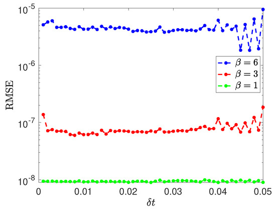
Figure 7. Example 2: Profile of RMSE versus time step for different values of $\beta$.

In Table 3, we also show that our method works very well for different time instances and with different values of the parameter $\beta$. We set the spatial mesh size to $\delta x=0.01.$

Table 3. Example 2: Error estimates at different time instnaces for different values of $\beta$.

$\mathit{\beta }$	T	RMSE	${\mathit{l}}_{\mathit{\infty }}$
	1	3.185 × ${10}^{-11}$	1.573 × ${10}^{-10}$
1	2	8.462 × ${10}^{-11}$	2.901 × ${10}^{-10}$
	3	1.143 × ${10}^{-9}$	5.811 × ${10}^{-9}$
	1	5.973 × ${10}^{-8}$	5.450 × ${10}^{-7}$
3	2	5.240 × ${10}^{-7}$	6.302 × ${10}^{-6}$
	3	4.073 × ${10}^{-6}$	7.026 × ${10}^{-5}$
	1	3.916 × ${10}^{-6}$	2.326 × ${10}^{-5}$
6	2	5.428 × ${10}^{-6}$	5.832 × ${10}^{-5}$
	3	1.425 × ${10}^{-4}$	1.815 × ${10}^{-3}$

Additionally, the profile of RMSE versus mesh size of the spatial domain is depicted in Figure 8. These results obtained for $\beta =1$ demonstrate that the choice of spatial mesh size does not significantly affect the accuracy of the method.

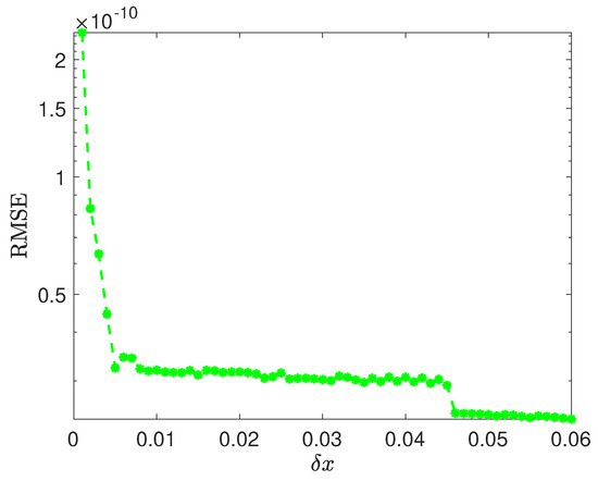
Figure 8. Example 2: Profile of RMSE versus $\delta x$.

Example 3. 

Consider the Fisher–KPP Equations (1)–(3) in 2D with $D=\alpha =\beta =1$ where $u_0, f,$ and g are obtained from the following analytical solution [17]:

$$\begin{array}{c}\hfill u(x,y,t)={\displaystyle \frac{1}{{\left(1+e^{\frac{\left(\frac{x-y}{\sqrt{2}}-\frac{5}{\sqrt{6}}t\right)}{\sqrt{6}}}\right)}^2}},(x,y)\in \mathsf{\Omega },0<t\le T.\end{array}$$

We first solve this problem on the domain $[-1,1]\times [-1,1]$ using our approach and compare the results with those from the wavelet collocation method [17]. Table 4 presents the $l_{\infty }$ errors for descending time step sizes using both the MPS-PBF and the wavelet collocation method. Our method consistently achieves higher accuracy with lower computational cost in terms of CPU time.

Table 4. Example 3: Comparison of $l_{\infty }$ error from wavelet collocation method [17] and MPS-PBF method.

	Wevlet Collocation		MPS-PBF
$\mathit{\delta }\mathit{t}$	${\mathit{l}}_{\infty }$	CPU Time	${\mathit{l}}_{\infty }$	CPU Time
$1/8$	9.576 × ${10}^{-5}$	20.86	6.526 × ${10}^{-8}$	4.92
$1/16$	2.391 × ${10}^{-5}$	37.39	5.755 × ${10}^{-9}$	6.82
$1/32$	5.976 × ${10}^{-6}$	70.11	3.657 × ${10}^{-9}$	13.10
$1/64$	1.494 × ${10}^{-6}$	136.26	6.779 × ${10}^{-9}$	25.23
$1/128$	3.734 × ${10}^{-7}$	268.76	5.756 × ${10}^{-9}$	39.88

Additionally, the problem is solved on a larger domain, $[-10,10]\times [-10,10]$. The profiles of the exact and approximate solutions are shown in Figure 9a,b, respectively. Figure 9c,d present the approximate solution and the corresponding error distribution, which is false-colored by the magnitude of the error. It is observed that, on the larger domain $[-10,10]\times [-10,10]$, the maximum absolute error is approximately 1 × ${10}^{-4}$, which is higher than the error obtained for the smaller domain $[-1,1]\times [-1,1]$.

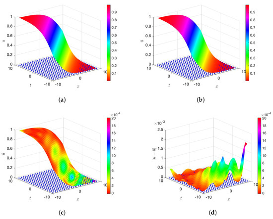
Figure 9. Example 3: Profiles of exact and approximate solutions and absolute error. (a) Exact Solution. (b) Approximate Solution. (c) Error on the surface of the approximate solution. (d) Error on the domain.

So far, we have considered the unit square domain while solving this time-dependent nonlinear problem. We now extend the study to several irregular computational domains commonly used in the meshless literature. As shown in Table 5, the MPS-PBF method demonstrates very high accuracy in solving the problem across these different irregular domains.

Table 5. Example 3: RMSE and $l_{\infty }$ for different computational domains.

Domains	${\mathit{n}}_{\mathit{i}}$	${\mathit{n}}_{\mathit{b}}$	RMSE	${\mathit{l}}_{\mathit{\infty }}$
Amoeba-shaped	876	250	1.601 × ${10}^{-9}$	2.752 × ${10}^{-8}$
Cassini-shaped	881	250	3.058 × ${10}^{-10}$	2.201 × ${10}^{-9}$
Star-shaped	895	250	1.143 × ${10}^{-9}$	2.293 × ${10}^{-8}$
L-shaped	878	250	6.354 × ${10}^{-11}$	4.657 × ${10}^{-10}$
Gear-shaped	889	250	5.133 × ${10}^{-9}$	7.925 × ${10}^{-8}$

In the preceding examples, we have considered only homogeneous initial–boundary value problems with Dirichlet boundary conditions. In the final example, we examine a nonhomogeneous mixed boundary value problem to evaluate the effectiveness of the proposed scheme.

Example 4. 

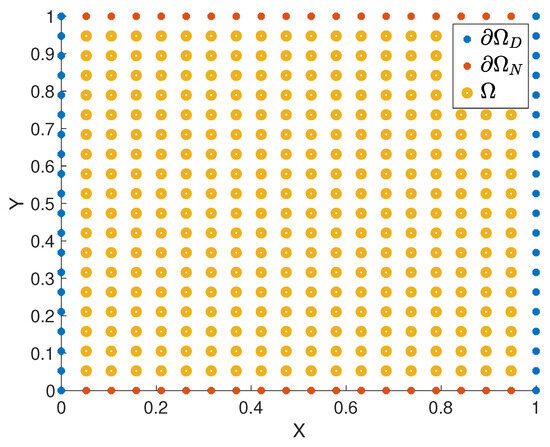
Consider the Fisher–KPP Equations (1)–(3) in 2D with $D=0.01,\alpha =0.148,\beta =1$, and the mixed boundary condition

$$u(x,y,t)=g_1(x,y,t),(x,y)\in \partial {\mathsf{\Omega }}_D,0<t\le T,$$

(17)

$${\displaystyle \frac{\partial u}{\partial y}}=g_2(x,y,t),(x,y)\in \partial {\mathsf{\Omega }}_N,0<t\le T,$$

(18)

where f, $u_0$, $g_1$, and $g_2$ are obtained from the following analytical solution [18]:

$$\begin{array}{c}\hfill u(x,y,t)={\displaystyle \frac{1}{2}}{e}^{-t}sin\left(\pi x\right)(1+cos\left(\pi y\right)),(x,y)\in \mathsf{\Omega },0<t\le T.\end{array}$$

Note that $\partial {\mathsf{\Omega }}_D,\partial {\mathsf{\Omega }}_N$ are the boundaries for Dirichlet and Neumann conditions, respectively, such that $\partial \mathsf{\Omega }=\partial {\mathsf{\Omega }}_D\cup \partial {\mathsf{\Omega }}_N$ as depicted in Figure 10.

Figure 10. Example 4: Profile of computational domain.

This problem is solved on a unit square domain using both uniform and nonuniform collocation nodes. For this experiment, we use $n_i=324$ interior nodes and $n_b=76$ boundary nodes. Table 6 presents the RMSE and $l_{\infty }$ errors for various time step sizes at the time instance $T=1$. Numerical results demonstrate that our scheme yields stable results across different time steps.

Table 6. Example 4: Comparison of RMSE and $l_{\infty }$ for uniform and non-uniform distribution of collocation nodes for various time steps at terminal time $T=1$.

	Uniform Collocation Nodes		Non Uniform Collocation Nodes
$\mathit{\delta }\mathit{t}$	RMSE	${\mathit{l}}_{\infty }$	RMSE	${\mathit{l}}_{\infty }$
0.03	1.671 × ${10}^{-9}$	9.386 × ${10}^{-7}$	1.031 × ${10}^{-9}$	6.528 × ${10}^{-7}$
0.05	3.348 × ${10}^{-9}$	8.789 × ${10}^{-7}$	2.562 × ${10}^{-9}$	6.087 × ${10}^{-7}$
0.07	1.832 × ${10}^{-9}$	7.602 × ${10}^{-7}$	2.755 × ${10}^{-9}$	5.393 × ${10}^{-7}$
0.09	2.218 × ${10}^{-9}$	5.808 × ${10}^{-7}$	1.936 × ${10}^{-9}$	3.660 × ${10}^{-7}$
0.11	3.983 × ${10}^{-9}$	5.133 × ${10}^{-7}$	2.839 × ${10}^{-9}$	4.260 × ${10}^{-7}$

Next, we solve this problem using uniformly distributed collocation nodes for different time instances with $\delta t=0.03$, as presented in Table 7. From the table, it can be observed that the numerical solutions at various time instances are highly accurate. These results are consistent with the findings from the previous examples and clearly demonstrate the effectiveness of the proposed MPS-PBF approach for solving the nonhomogeneous Fisher–KPP equation with mixed boundary conditions as well.

Table 7. Example 4: Error estimates at different terminal time.

T	$\mathit{RMSE}$	${\mathit{l}}_{\mathit{\infty }}$
1	8.997 × ${10}^{-8}$	9.375 × ${10}^{-7}$
3	8.877 × ${10}^{-7}$	1.163 × ${10}^{-5}$
5	7.219 × ${10}^{-6}$	9.760 × ${10}^{-5}$
7	1.227 × ${10}^{-5}$	1.712 × ${10}^{-4}$
10	3.951 × ${10}^{-5}$	5.326 × ${10}^{-4}$

4. Conclusions and Future Work

In this work, we have computed the numerical solution of the nonlinear Fisher–KPP equation using a space–time collocation method based on the MPS-PBF approach. The proposed scheme offers significant advantages in terms of flexibility, adaptability, and the ability to handle complex geometries. It is well known that, unlike radial basis function methods, the MPS-PBF formulation eliminates the need for an optimal shape parameter and has been shown in the literature to achieve superior accuracy [10]. In this comparative analysis, we further confirm that our proposed approach demonstrates both high accuracy and stability relative to established techniques such as the BDF3 and wavelet collocation methods. Numerical experiments demonstrate excellent performance at smaller time instances; however, the accuracy gradually deteriorates over longer time intervals. Future research will focus on developing a hybrid numerical scheme to enhance long-time accuracy and extending the methodology to a broader class of nonlinear reaction–diffusion equations.

References

- Fisher, R.A. The wave of advance of advantageous genes. Ann. Eugenes 1937, 7, 353–369. [Google Scholar] [CrossRef]
- Kolmogorov, A.N.; Petrovskii, I.P.; Piskunov, N.S. A study of the diffusion equation with increase in the amount of substance, and its application to a biological problem. In Selected Works of A.N. Kolmogorov I; Tikhomirov, V.M., Ed.; Volosov, V.M., Translator; Kluwer: Dordrecht, The Netherlands, 1937; pp. 248–270. ISBN 90-277-2796-1. [Google Scholar]
- Murray, J.D. Mathematical Biology: An Introduction; Springer: Berlin/Heidelberg, Germany, 1993. [Google Scholar]
- Macias-Diaz, J.E. A bounded finite-difference discretization of a two-dimensional diffusion equation with logistic nonlinear reaction. Int. J. Mod. Phys. C 2011, 22, 953–966. [Google Scholar] [CrossRef]
- Khiari, N.; Omrani, K. Finite difference discretization of the extended Fisher-Kolmogorov equation in two dimensions. Comput. Math. Appl. 2011, 62, 4151–4160. [Google Scholar] [CrossRef]
- Vimal, V.; Sinha, R.K.; Pannikkal, L. Numerical Methods for Solving Nonlinear Fisher Equation using Backward Differentiation Formula. Int. J. (AAM) 2024, 19, 4. [Google Scholar]
- Tang, S.; Weber, R.O. Numerical study of Fisher’s equation by a Petrov-Gelerkin finite element method. J. Austral. Math. Soc. Ser. B 1991, 33, 27–38. [Google Scholar] [CrossRef]
- Roessler, J.; Hussner, H. Numerical solution of the 1 + 2 dimensional Fisher’s equation by finite elements and Galerkin method. Mathl. Comput. Model. 1997, 25, 57–67. [Google Scholar] [CrossRef]
- Chen, C.S.; Fan, C.M.; Wen, P.H. The method of particular solutions for solving certain partial differential equations. Numer. Methods Partial. Differ. Equ. 2012, 28, 506–522. [Google Scholar] [CrossRef]
- Dangal, T.; Chen, C.S.; Lin, J. Polynomial particular solutions for solving elliptic partial differential equations. Comput. Math. Appl. 2017, 73, 60–70. [Google Scholar]
- Dangal, T.; Khatri Ghimire, B.; Lamichhane, A.R. Localized method of particular solutions using polynomial basis functions for solving 2D nonlinear partial differential equations. Partial. Differ. Equ. Appl. Math. 2021, 4, 100114. [Google Scholar] [CrossRef]
- Yao, G.; Kolibal, J.; Chen, C.S. A localized approach for the method of approximate particular solutions. Comput. Math. Appl. 2011, 61, 2376–2387. [Google Scholar] [CrossRef]
- Zhang, X.; Yao, L.; Liu, J. Numerical study of Fisher’s equation by the RBF-FD method. Appl. Math. Lett. 2021, 120, 107195. [Google Scholar] [CrossRef]
- Hamaidi, M.; Naji, A.; Charafi, A. Space–time localized radial basis function collocation method for solving parabolic and hyperbolic equations. Eng. Anal. Bound. Elem. 2016, 67, 152–163. [Google Scholar] [CrossRef]
- Cao, Y.; Chen, C.S.; Zheng, H. Space-time polynomial particular solutions method for solving time-dependent problems. Numer. Heat Transf. Part B Fundam. 2019, 77, 181–194. [Google Scholar] [CrossRef]
- Liu, C.S. A multiple scale Trefftz method for an incomplete Cauchy problem of biharmonic equation. Eng. Anal. Bound. Elem. 2013, 37, 17–42. [Google Scholar] [CrossRef]
- Oruç, Ö. An efficient wavelet collocation method for nonlinear two-space dimensional Fisher–Kolmogorov–Petrovsky–Piscounov equation and two-space dimensional extended Fisher–Kolmogorov equation. Eng. Comput. 2020, 36, 839–856. [Google Scholar] [CrossRef]
- Achouri, T.; Ayadi, M.; Habbal, A.; Yahyaoui, B. Numerical analysis for the two-dimensional Fisher–Kolmogorov–Petrovski–Piskunov equation with mixed boundary condition. J. Appl. Math. Comput. 2022, 68, 3589–3614. [Google Scholar] [CrossRef]
Disclaimer/Publisher’s Note: The statements, opinions and data contained in all publications are solely those of the individual author(s) and contributor(s) and not of MDPI and/or the editor(s). MDPI and/or the editor(s) disclaim responsibility for any injury to people or property resulting from any ideas, methods, instructions or products referred to in the content. |
© 2025 by the authors. Licensee MDPI, Basel, Switzerland. This article is an open access article distributed under the terms and conditions of the Creative Commons Attribution (CC BY) license (https://creativecommons.org/licenses/by/4.0/).