Abstract
To address the key challenges in shortest path planning for known static obstacle maps—such as the tendency to converge to local optima in U-shaped/narrow obstacle regions, unbalanced computational efficiency, and suboptimal path quality—this paper presents an enhanced Artificial Lemming Algorithm (DMSALAs). The algorithm integrates a dynamic adaptive mechanism, a hybrid Nelder–Mead method, and a localized perturbation strategy to improve the search performance of ALAs. To validate DMSALAs efficacy, we conducted ablation studies and performance comparisons on the IEEE CEC 2017 and CEC 2022 benchmark suites. Furthermore, we evaluated the algorithm in mobile robot path planning scenarios, including simulated grid maps (10 × 10, 20 × 20, 30 × 30, 40 × 40) and a real-world experimental environment built by our team. These experiments confirm that DMSALAs effectively balance optimization accuracy and practical applicability in path planning problems.
MSC:
68W50
1. Introduction
Meta-heuristic (MH) algorithms excel at solving complex optimization problems like mobile robot path planning in static environments, where traditional methods struggle with non-convex obstacle avoidance and high-dimensional search spaces. Their ability to balance global exploration (finding feasible paths around fixed obstacles) and local exploitation (optimizing path length) makes them particularly suitable for grid-based navigation systems. The No Free Lunch theorem [1] further justifies developing specialized variants for structured environments with predetermined obstacle configurations.
Recently, the field of MH algorithms has witnessed a remarkable increase in research focus and attention. There are many types of MH algorithms, including swarm intelligence algorithms, evolutionary algorithms, and physics-inspired algorithms. There are many swarm intelligence algorithms; for example, the improved gorilla troops optimizer (IGTO) [2] represents a novel meta-heuristic approach that integrates lens opposition and adaptive hill strategies. The Horse Herd Optimization Algorithm (HOA) [3] derives from observed social behaviors in equine populations, systematically encoding six characteristic traits across growth phases. The Graylag Goose Optimization Algorithm (GGO) [4] computationally emulates the self-organizing flight patterns of geese that emerge from altitude and meteorological variations. Binary variants of the Artificial Bee Colony algorithm (BABC) [5] preserve the defined criteria while inheriting the advantages of the original ABC algorithm. The Modified Artificial Hummingbird Algorithm (MAHA) [6] improves upon the performance of its predecessor. The Whale Optimization Algorithm (WOA) [7] is inspired by the bubble-net hunting strategy, which can precisely circumvent obstacles along local paths. The hybrid gray wolf optimization (HGWO) [8,9,10] utilizes combined metaheuristic principles to generate collision-free optimal paths for autonomous robots. The improved PSO (IPSO) [11] improves the performance of autonomous path planners by optimizing 3D route generation for speed and precision. The improvement adaptive ant colony algorithm (IAACO) [12] integrates four key factors—directional guidance, obstacle exclusion, adaptive heuristic information, and adjustable pheromone decay to optimize indoor robotic path planning. The proposed algorithm, named the hybrid Particle Swarm Optimization-Simulated Annealing algorithm [13,14], successfully avoids local optima entrapment and enhances search diversity, resulting in quicker convergence and decreased resource consumption. Each of these algorithms possesses distinct characteristics. For example, the IGTOs algorithm exhibits strong exploration capability, excellent balance, and high robustness; however, it suffers from increased computational complexity and requires careful parameter tuning. Similarly, the WOAs algorithm offers a simple structure, ease of implementation, and strong local exploitation ability, yet it is prone to premature convergence and demonstrates limited global exploration performance. Evolutionary algorithms include many algorithms, such as the Population State Evaluation-based Differential Evolution (PSEDEs) [15], which incorporates insights from the evolutionary states of Differential Evolution (DEs), and the enhanced Genetic Algorithm (EGAs) [15,16], which focuses on advancing path initialization techniques in continuous space, ultimately deriving the best-performing route between given start and goal coordinates. The PSEDEs algorithm features a simple structure and ease of implementation, with strong local exploitation capability and fast convergence speed. However, it is prone to receiving traps in local optima, and its search behavior heavily depends on population distribution. The EGAs algorithm demonstrates robust global exploration ability and low dependency on specific problem structures, yet it suffers from slow convergence and high sensitivity to parameter settings. In addition to the above two algorithms, there are also physics-inspired algorithms, for example, the Multi-Strategy Boosted Snow Ablation Optimizer (MSAO) [16] presents a new SAO version enhanced by four optimization strategies. The Interior Search algorithm (ISA) [17] takes methodological cues from harmonic balance concepts in decor composition. The Farmland Fertility algorithm (FFAs) [18] computationally models the productivity cycles inherent in arable land biomes. The MSAOs algorithm features a novel search mechanism with clear physical intuition, yet it suffers from insufficient exploitation capability. The ISAs algorithm incorporates a unique update mechanism but is prone to receiving traps in local optima. The FFAs algorithm exhibits a strong metaphorical foundation and adaptability, along with robust global exploration ability; however, it has weaknesses in local exploitation and requires careful parameter tuning. These original and improved algorithms leverage various strategies, such as Levy flight [19] can improve the global search efficiency of robots in sparse obstacle environments, bidirectional search strategy [20] is capable of narrowing down the search scope and decreasing the time required to identify the optimal trajectory, and adaptive parameters strategy [21] can use a feedback mechanism to achieve dynamic adaptation of parameters, thereby improving the quality of the current path solution. However, many algorithms perform well in dynamic environments, but when optimizing paths for fixed maps, they suffer from excessive exploration (such as unnecessary random walking) or lack a directional search mechanism for known obstacle structures, resulting in suboptimal path lengths.
The ALAs [22] represents an innovative swarm intelligence algorithm inspired by lemming behaviors: migratory patterns, burrowing activities, and food-searching strategies. The proposed method exhibits a straightforward architecture, implementation simplicity, and superior computational performance. It incorporates Brownian motion, random walk, and Levy flight mechanisms to achieve exploration-exploitation equilibrium, while adaptive parameter tuning progressively narrows the search range with iterations. However, the algorithm has certain limitations, including fixed parameters for search radius and jump probability, a lack of an adaptive mechanism to dynamically adjust based on population diversity or iteration progress, and an absence of a local fine-tuning strategy for the current optimal solution, which may lead to entrapment in local optima. Additionally, population diversity may decline rapidly with iterations, resulting in premature convergence. Especially when applied to mobile robot path planning problems, the ALAs algorithm further exposes the following issues: a fixed search radius makes it prone to generating collision paths in dense obstacle areas, a lack of heuristic guidance for known map structures (prioritizing search along obstacle contours), and a decline in population diversity causes path optimization to prematurely converge to suboptimal solutions.
The aforementioned algorithms have been widely applied in various research domains. However, when employed for path planning problems, they commonly face challenges such as an imbalance between exploration and exploitation, weak local search capability, and a tendency toward premature convergence—issues that also apply to the ALAs algorithm. To systematically address these limitations, this study addresses the optimal path planning problem in predefined static obstacle environments, with its primary challenges including: ensuring global optimal pathfinding within bounded constraint spaces, avoiding algorithmic entrapment in local optima within U-shaped or narrow obstacle regions, and striking a balance between computational efficiency and path optimality. To tackle these limitations, we introduce DMSALAs, which integrate a dynamic adaptive mechanism, hybrid Nelder–Mead optimization, and localized perturbation strategies to boost the search efficiency of the ALAs algorithm in path planning for mobile robots within static obstacle environments. The dynamic adaptive mechanism is designed to modulate the search granularity according to the proximity between the current trajectory and obstacles. The Hybrid Nelder–Mead optimization is employed for local smoothing of key turning points in the path. The small-range perturbation can conduct directional exploration for dead-end exits (such as the openings of U-shaped obstacles).
To verify the performance of the DMSALAs algorithm, we conducted a series of comprehensive experimental evaluations. First, to evaluate the efficacy of the three strategies, we performed ablation studies on the IEEE CECs 2017 benchmark, comparing results with six variant algorithms. Both IEEE CECs 2017 and CECs 2022 benchmarks were utilized to comprehensively assess DMSALAs against eight state-of-the-art algorithms spanning different categories. Furthermore, to explore the algorithm’s performance in mobile robot path planning, we set the shortest path as the optimization goal. DMSALAs were tested on four maps with varying dimensions (10 × 10, 20 × 20, 30 × 30, and 40 × 40), along with the real-world experimental setup constructed by our team. All experimental results effectively validated the superiority of the DMSALAs algorithm. This study provides a new solution for path length optimization based on prior maps in static environments, and its improved strategies specifically perform collaborative optimization for convergence speed and path optimality in structured obstacle spaces.
2. ALA Algorithm
ALAs primarily models key behaviors of lemmings, as depicted in Figure 1.

Figure 1.
ALAs mainly simulation three behaviors of lemmings. (a) long-distance migration; (b) digging holes; (c) foraging behavior.
2.1. Initialization
In the initialization phase, similar to other algorithms, the algorithm generates an ini-tial solution randomly within a predefined solution space ,
is the population size and
is a dimension. The formula is as follows:
where , , , and is the upper and lower boundaries.
2.2. Long-Distance Migration (Exploration)
The formula of lemmings’ long-distance migration is as follows:
where and are the location of search agent at and iteration. is the current optimal solution. , as is shown in Equation (5). is a random number uniformly distributed within the interval [−1, 1]. It determines, at each iteration, whether an individual is more inclined to move toward the best solution or to random exploration. When approaches 1, the weight of the term increases, enhancing the exploitation behavior and causing the individual to closely follow the current best solution. When approaches −1, the weight of the term increases due to the growing value of , thereby strengthening the exploration behavior and promoting random walks within the search space. In this way, adaptively adjusts the balance between exploration and exploitation for each individual at every iteration, rather than relying on a fixed strategy. is the flag for the search direction conversion, as is shown in Equation (3). This introduces a stochastic reverse mechanism into the search process. When the individual moves in the original direction determined by the subsequent vector; when , the individual moves in the opposite direction. This mechanism effectively prevents individuals from blindly persisting in a single direction and enhances the likelihood of escaping local optima. It is a random vector representing Brownian motion; its value follows the probability density of a standard normal distribution and primarily controls the step size. acts as a random multiplicative factor applied to the entire movement vector. A larger value results in a significant jump, while a smaller B value leads to a fine–grained local move. interacts with the product jointly determines the basic step size and direction of the current movement. This base random step is then combined with the exploration-exploitation directional vector weighted by , ultimately determining the position update, as is shown in Equation (4). represents a randomly chosen individual within the population, is an integer between 1 and .
2.3. Digging Holes (Exploration)
The secondary behavior of lemmings entails burrowing to achieve dual purposes: self-protection and food storage. The corresponding model is described below:
where , is a randomly generated step size that periodically oscillates within the interval [0, 2). The exploration step size expands during iterations when the sine function approaches 1, and contracts when the sine function approaches −1; however, due to the addition of 1, the minimum value remains non-negative. This mechanism helps balance global search capability with the avoidance of excessive jumps. represents a randomly chosen individual from the population, is an integer between 1 and . Through the coordinated interaction of oscillating random step size, stochastic direction reversal, and the base random vector, the model effectively implements a comprehensive, randomized exploration strategy with adaptive step-size variation.
2.4. Foraging (Exploitation)
The third behavior of lemmings involves foraging, wherein they move around within their burrows to locate food. The formula is as follows:
where is for spiral foraging, as is shown in Equation (7). is the search radius, as is shown in Equation (8). This equation generates a local search behavior characterized by a random spiral trajectory around the optimal solution through the coordinated action of the function and . controls the scale of the spiral, while the combination of trigonometric functions determines its specific shape and phase. Together, these components enable the spiral function to dynamically generate a spiral vector whose amplitude is proportional to the distance and whose shape varies randomly, guiding individuals in conducting fine-grained and diverse exploration around the optimal solution.
2.5. Exploration and Exploitation Transition Mechanism
The transition mechanism between exploration and exploitation is governed by the energy coefficient .
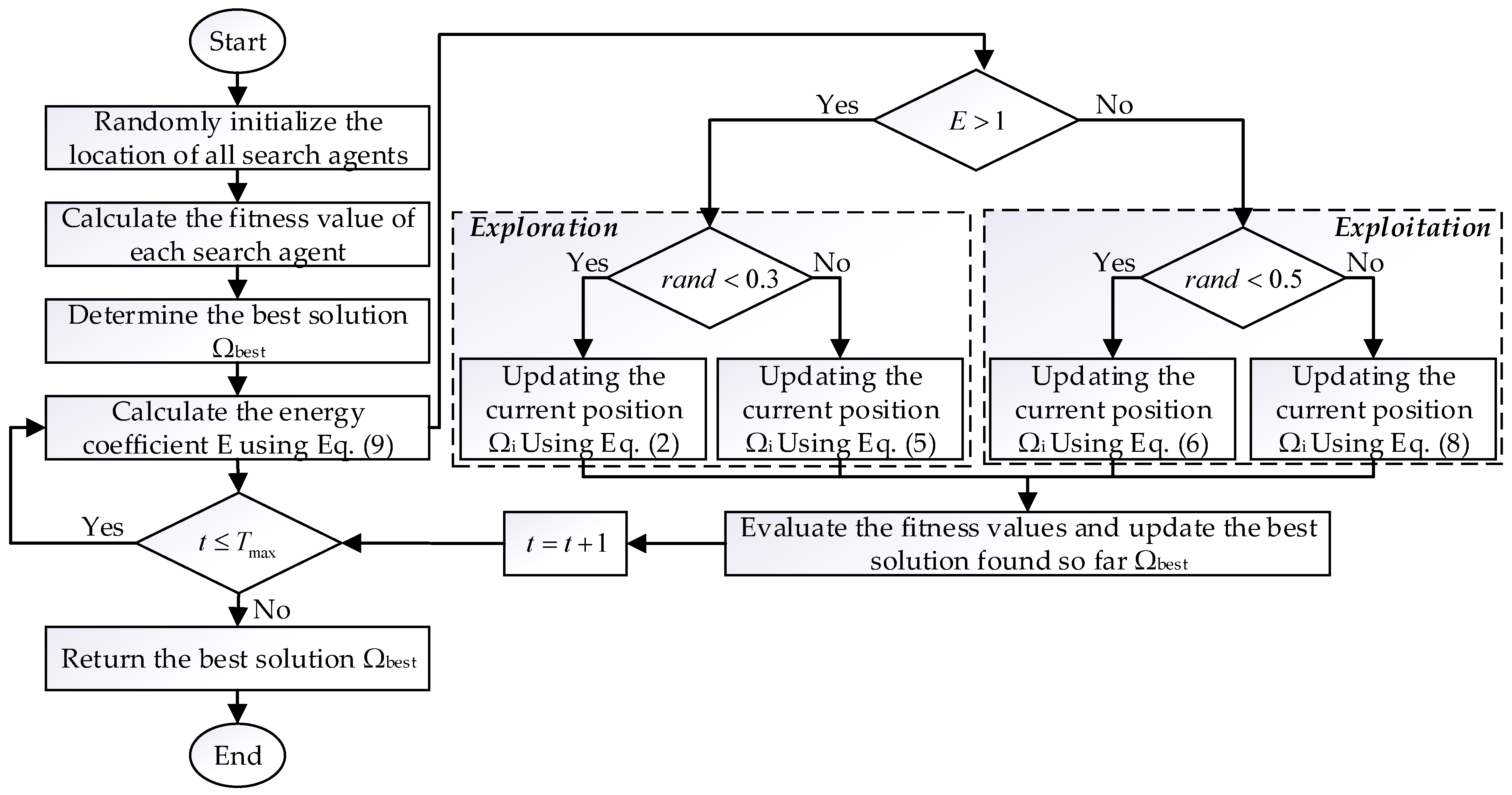
In the initialization phase of ALAs, some control parameters were set. Afterwards, at each iteration, if the energy coefficient , ALAs enter the exploration phase, executing long-distance migration behavior or digging behavior. When , ALAs perform exploitation through foraging behavior or evading natural predators’ behavior. These behaviors are employed by all search agents to update new candidate solutions and determine the currently found optimal solution. As the number of iterations increases, the value of gradually decreases, allowing search agents to transition robustly from exploration to exploitation. Once the termination condition is satisfied, the procedure will terminate and output the optimal global solution. DMSALAs workflow is shown in Figure 2.
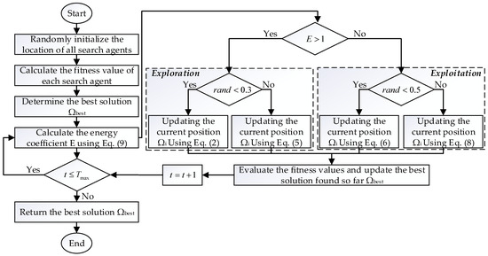
Figure 2.
DMSALAs workflow.
3. Improvement Strategy
In this section, we implement a dynamic adaptive mechanism, a hybrid Nelder–Mead approach, and a localized perturbation strategy to improve the search performance of the ALAs algorithm.
3.1. Dynamic Adaptive Mechanism
The original algorithm features a fixed search radius and jump probability, resulting in poor robustness [23]. Consequently, we introduce an exponentially attenuating radius to enable the DMSALAs algorithm to dynamically adjust its search radius and jump probability [24,25], thereby achieving adaptability to different problem characteristics. The formula is presented as follows:
where the maximum search radius is an Euclidean norm expressed as , where the minimum search radius is , and the radius decay coefficient is . Let and denote the current and maximum number of objective function evaluations.
In the initial stage, when , , so the search radius . This allows the mobile robot to explore possible paths in a large area, and in the Late stage of algorithm search, , , , causing . The algorithm then prioritizes local fine-grained search, enabling the robot to fine-tune around the discovered suboptimal paths and converge near the optimal solution. The search radius decays exponentially with the number of evaluations , scanning the environment on a large scale using the map’s diagonal length in the early stage, and optimizing paths with level precision in the late stage.
3.2. The Hybrid Nelder–Mead Method
To strengthen the algorithm’s aptitude for local search, we incorporate the hybrid Nelder–Mead method into the ALAs algorithm [26,27]. The hybrid Nelder–Mead method enables adaptive local search and an elite retention strategy, replaces inferior solutions with superior ones, and prevents population degradation [28]. The pseudocode for the Hybrid Nelder–Mead Method is as follows (Algorithm 1):
where worst_index denotes the encoded address of the current suboptimal solution, new_position signifies the optimal outcome of the local search process, and new_fitness stands for the corresponding objective function value.
| Algorithm 1. Pseudocode for the Hybrid Nelder–Mead Method |
| IF current_Fes > 0.7 · max_Fes AND mod (current_Fes 5) = 0 THEN // Perform local search using fminsearch [new_position, new_fitness] = fminsearch(objective_function, current_position) IF new_fitness < current_fitness THEN // Update current individual current_position = new_position global_best_fitness = new_fitness // Find worst individual in population worst_index = index_of_max(fitness_population) // Replace worst individual with new solution population[worst_index] = new_position fitness_population[worst_index] = new_fitness END IF END IF |
In the late phase of the algorithm, a hybrid Nelder–Mead approach is integrated, with the primary aim of enhancing the quality and convergence accuracy of mobile robot path planning results. Specifically, the Nelder–Mead simplex method is employed to conduct fine-grained searches on the current global optimal path (current_position), enhancing the algorithm’s exploitation capability to improve convergence precision and the quality of the solved path. Meanwhile, population diversity is maintained by replacing the worst path in the population.
When current_Fes > 0.7 max_Fes, it signifies that the algorithm has entered the terminal phase of iteration. Additionally, mod (current_Fes, 5) = 0 means the current evalution number current_Fes is divisible by 5. When both conditions current_Fes > 0.7 max_Fes and mod (current_Fes, 5) = 0 are satisfied, a gradient-free Nelder–Mead local search is performed once every five evaluations. This strategy substantially cuts down the algorithm’s computational overhead while guaranteeing the quality of path planning results.
During local search, the fminsearch function is used, which takes the objective function fobj, the current global optimal path (current_position). This strategy substantially cuts down the algorithm’s computational overhead while guaranteeing the quality of path planning results. If the fitness value of the new path obtained through local enhancement search is superior to that of the current global optimal path (new_fitness < global_best_fitness), the global optimal path (current_position) and its fitness value Score are updated. This indicates that a better path for the mobile robot has been found, which is then taken as the new global optimal path.
Next, the new path and fitness value new_fitness obtained from fminsearch are used to replace the worst path in the population. Specifically, the fitness values of all paths within the population are computed using the max function to determine the index of the least optimal path. The coordinate values and fitness value of this worst path are then replaced by the new path P and new_fitness. This procedure iteratively discards suboptimal path solutions to enhance the overall quality of the population.
3.3. Small-Range Perturbation Strategy
To address the ALAs algorithms’ propensity to converge to local optima, we devised a localized perturbation strategy [29] grounded in an evaluation of the current population diversity. The formula is presented as follows:
The maximum jump probability is , and the minimum jump probability is . To characterize the distribution of the population within the solution space and identify premature convergence of the ALAs algorithm, the standard deviation of each column of is calculated as . A larger standard deviation indicates greater individual differences in that dimension (better population diversity). The average standard deviation across all dimensions is , representing the overall average diversity of the population across all dimensions.
When the path distribution is concentrated (), a 10% basic perturbation is retained; when the distribution is dispersed (), the perturbation intensity is increased to 50%. This mechanism ensures that mobile robots can quickly locate feasible paths in complex environments and eliminate unnecessary jitter during the convergence phase.
When the path distribution is dispersed (), maintaining a 50% perturbation intensity to achieve a high jump probability. When the path distribution is concentrated (), , reducing the jump probability while retaining 10% basic perturbation to prevent the algorithm from falling into local optima. This mechanism ensures that mobile robots can both quickly locate feasible paths in complex environments and eliminate unnecessary jitter during the convergence phase. The formula is as follows:
3.4. DMSALAs Flow
The workflow of DMSALAs in mobile robot path planning is as follows:
- (a)
- Initialization Phase:
Set the initial global optimal fitness value Score = inf, indicating no optimal path solution has been found yet. Initialize the global optimal position as a zero vector , indicating that path fitness has not been evaluated. Initialize the convergence curve storage parameter to record the algorithm’s convergence characteristics during iterations.
- (b)
- Initial Fitness Evaluation:
Initialize the evaluation counter and the global optimal path cost Score. Decode each path in the population and compute its comprehensive performance using the fitness function fobj, which optimizes for path length.
- (c)
- Dynamic Adaptive Adjustment Mechanism:
Formulate a dynamic adaptation parameter to accommodate environmental dynamics encountered by the robot. Set a small-range perturbation factor to enable local path refinement.
- (d)
- Search Strategy Selection
Global Search ()
If , initiate a hybrid search combining the global best solution and a random individual to leverage historical information and random exploration. If , execute an adaptive step-size random walk for global sampling.
Local Search ()
If perform a constrained spiral search around the current position.
If further decide.
If apply an adaptive Levy flight strategy to perturb the current best path for escaping local optima.
If execute a small-range perturbation for fine-tuning the path.
- (e)
- New Path Evaluation:
Compute the fitness of new paths generated by both global and local searches using the objective function fobj. Apply a greedy strategy to compare new paths with the current best path, updating the solution if the new path is superior.
- (f)
- Nelder–Mead Local Enhancement:
When current_Fes > 0.7 max_Fes AND mod (current_Fes, 5) = 0 (after 70% of evaluations and every 5 iterations).
Invoke the fminsearch function with parameters fobj, current_position to perform gradient-free Nelder–Mead local search.
Substitute the least optimal individual in the population with the new trajectory and its fitness value to preserve diversity.
- (g)
- Termination and Output:
Upon completion of all iterations, the global optimal trajectory and its corresponding fitness value are recorded, followed by the output of the mobile robot’s optimal path plan.
3.5. Time Complexity Analysis
To analyze the time complexity of the DMSALAs algorithm, we adopt a standard methodology. Specifically, we use the first problem from the CEC 2017 benchmark suite, which has a dimensionality of 10. For consistency across all algorithms being compared, we set a maximum of 1000 iterations. The equation is evaluated using given below:
is the time taken by the first problem from the CEC 2017 benchmark suite (called CEC 2017 F1) for a single run, is the time taken by an algorithm for evaluating CEC 2017 F1 for five runs. The ratio reflects the relative difference between the single—run time and the time for five runs of an algorithm, normalized by the benchmark time . A larger ratio indicates a more significant discrepancy between these two-time metrics relative to . Thereby showcasing the variations in time complexity among different algorithms when solving this problem and highlighting the superior time-related performance and competitiveness of a specific algorithm compared to others.
For the DMSALAs algorithm, its ratio value is 5.089566. Among the tested algorithms, this places it in second position, just behind the GWOs algorithm. Notably, it surpasses the GAs and SFOAs algorithms. The time complexity analysis is presented in Table 1.

Table 1.
Time Complexity Analysis.
3.6. Parameter_Sensitivity_Analysis
To conduct parameter sensitivity analysis, we selected five test functions (F1, F7, F15, F23, and F30) from the CEC 2017 test suite, with a dimension of dim = 10 and a maximum fitness evaluation count of Maxfex = 1000 dim. Each function was independently run for 30 rounds. The values of the three parameters, namely the radius decay coefficient in the Dynamic Adaptive Mechanism, the maximum jump probability , and the population size , were set differently. The average solutions obtained by the DMSALAs algorithm on the five functions under various combinations of , , and are presented in Table 2 and Figure 3. The optimal value is highlighted with a red dot in Figure 3.

Table 2.
The average solutions obtained by the DMSALAs on five functions under various combinations of , , and .

Figure 3.
The solutions of the DMSALAs on 5 functions when , , and take different values.
The sensitivity analysis of the average fitness values under different parameter settings through system testing shows that when the parameter varies within the range of 1 to 10, DMSALAs’ performance remains relatively stable. The best performance is achieved when , with an average fitness value of 1677.95, which is not significantly different from other values (fluctuating between 1677.95 and 1682.84), indicating that the parameter has a minor impact on the algorithm’s performance within the tested range and demonstrates good robustness. The parameter exhibits a distinct sensitivity characteristic. As increases from 0.1 to 0.5, the average fitness value improves from 1681.26 to 1670.95, representing a performance enhancement of approximately 0.6%. However, when further increases to 0.9, the performance drops to 1686.48. This suggests that there is an optimal value (0.5), and exceeding this range leads to performance deterioration. The sensitivity analysis of the parameter indicates that the algorithm’s performance is optimal at = 30 (1672.61). As increases from 20 to 60, the performance shows an initial improvement followed by slight fluctuations, but the overall change is relatively small (1672.61–1678.60), indicating that the parameter has a limited impact on the algorithm’s performance within a reasonable range. The results of the sensitivity analysis suggest that all three parameters have some influence on the algorithm’s performance, but the degree and pattern of their influence vary. The DMSALAs can maintain the best performance when , , and .
4. Experimental Verifications
To verify the performance of the DMSALAs algorithm, we conducted a series of comprehensive experimental evaluations, encompassing an ablation study on the IEEE CEC 2017 benchmark and comparative assessments on both IEEE CEC 2017 and CEC 2022. To ensure fairness in algorithm evaluation, we employed the maximum number of fitness evaluations as the primary metric for assessing algorithm efficiency. We set and . To maintain consistency with the majority of existing studies and enable fair comparisons, the experiments primarily focus on the standard 30D setting on the IEEE CEC 2017 and 10D on the IEEE CEC 2022. This dimensionality is widely recognized as a benchmark for evaluating algorithm performance, as it strikes a favorable balance between problem complexity and computational cost.
All experimental results reported in this section are presented as statistical averages and standard deviations derived from 30 independent trial runs. The comparative analysis employs a sign test notation system, where ‘+’ denotes superior performance of a comparison algorithm over DMSALAs on a given test function, ‘− indicates inferior performance relative to DMSALAs, and ‘=‘ signifies statistically equivalent results. For a comprehensive performance evaluation, we implement Friedman’s test analysis, incorporating both average ranking scores and ordinal rankings. Before conducting the Friedman test, the Lilliefors normality test was performed on all results, and the corresponding p-values are presented in Table 3, Table 4 and Table 5. These dual metrics provide a quantitative assessment of each algorithm’s overall optimization capability across the benchmark suite. To enhance the credibility of our experimental results, we conducted the Wilcoxon rank-sum test for statistical significance analysis.

Table 3.
DMSALAs performance compared with its variants on IEEE CECs 2017.

Table 4.
DMSALAs performance compared with 8 advanced algorithms on IEEE CEC 2017.

Table 5.
DMSALAs performance compared with 8 advanced algorithms on IEEE CEC 2022.
4.1. Ablation Experiment
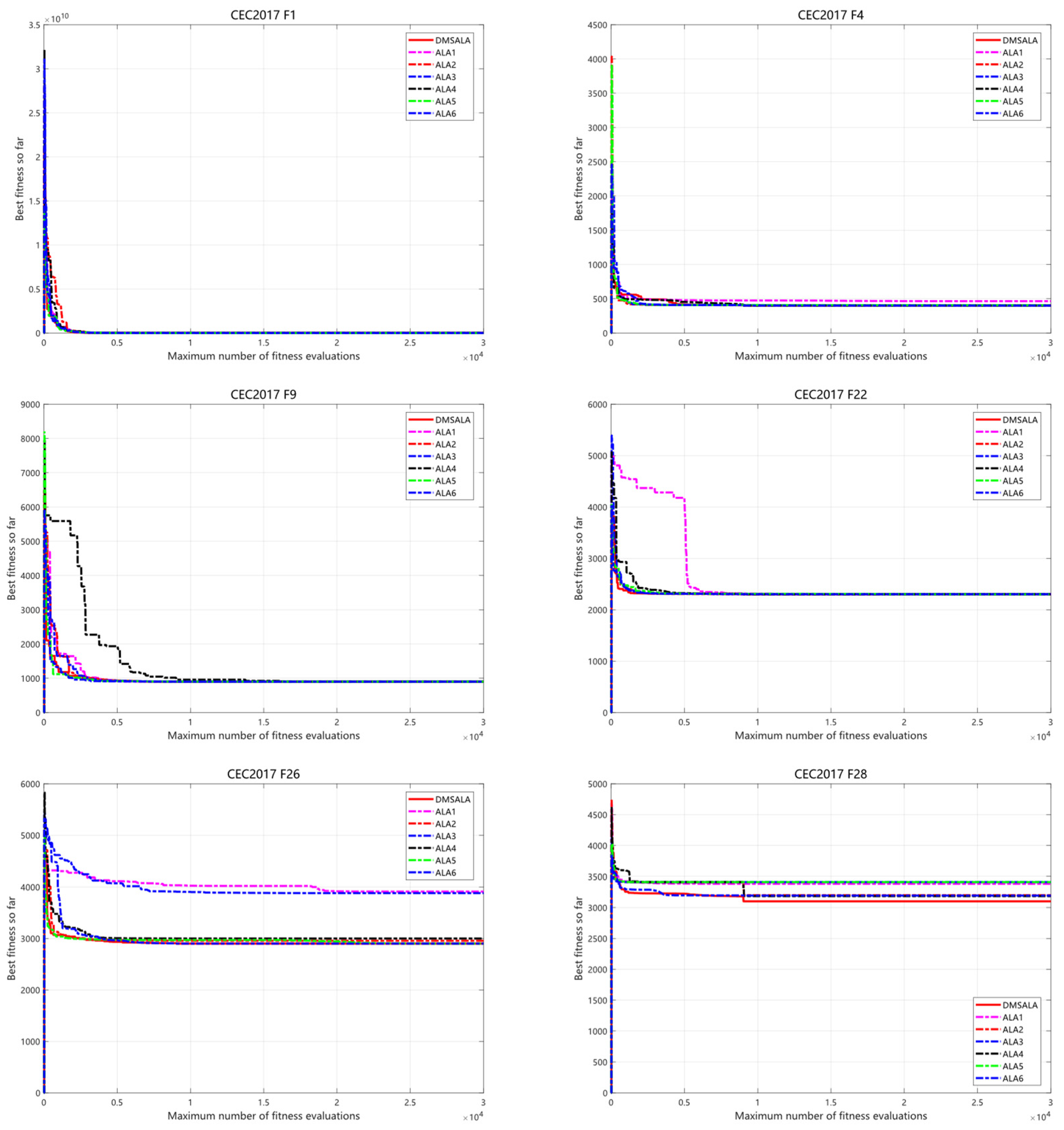
An ablation study was carried out using the IEEE CEC 2017 dataset to assess the performance of various strategies. Six variants of the ALAs algorithm, namely ALAs1–ALAs6, were designed, each integrating distinct strategies. Specifically, ALA1 features a dynamic adaptive mechanism; ALAs2 utilizes the hybrid Nelder–Mead approach; ALAs3 applies a small-scale perturbation technique; ALAs4 combines the dynamic adaptive mechanism with the hybrid Nelder–Mead method; ALAs5 integrates the dynamic adaptive mechanism and the small-scale perturbation strategy; and ALAs6 merges the hybrid Nelder–Mead approach and the small-scale perturbation technique.
As presented in Table 3, the results of the Lilliefors normality test are as follows: a total of 203 tests (29 test functions and seven algorithms), with 38 cases where the normal distribution cannot be rejected and 165 cases of non-normal distribution. These results confirm that our data indeed have significant non-parametric characteristics, thereby providing a sufficient statistical basis for the application of the Friedman test. The DMSALAs algorithm outperformed others by identifying 22 optimal solutions, with a (+/−/=) statistical outcome of (22/1/6) and a Friedman mean of 1.48, securing the top rank. Following closely, ALAs6 detected 17 optimal values, yielding a (+/−/=) statistic of (17/2/10) and a Friedman mean of 1.62, ranking second. ALAs5 identified five optimal values, with a (+/−/=) statistical result of (5/5/19) and a Friedman mean of 2.97, placing sixth. ALAs4 found six optimal solutions, recording a (+/−/=) statistic of (6/9/14) and a Friedman mean of 2.90, ranking fifth. ALAs3 recognized 11 optimal values, presenting a (+/−/=) statistical outcome of (11/7/11) and a Friedman mean of 2.55, ranking fourth. ALAs2 discovered 10 optimal solutions, with a (+/−/=) statistic of (10/4/15) and a Friedman mean of 2.34, ranking third. In contrast, ALAs1 only identified 10 optimal values, with a (+/−/=) statistical result of (3/11/15) and a Friedman mean of 3.52, ranking seventh. These findings not only validate the effectiveness of the three strategies mentioned above but also emphasize the remarkable superiority of the DMSALAs algorithm, as depicted in Figure 4.
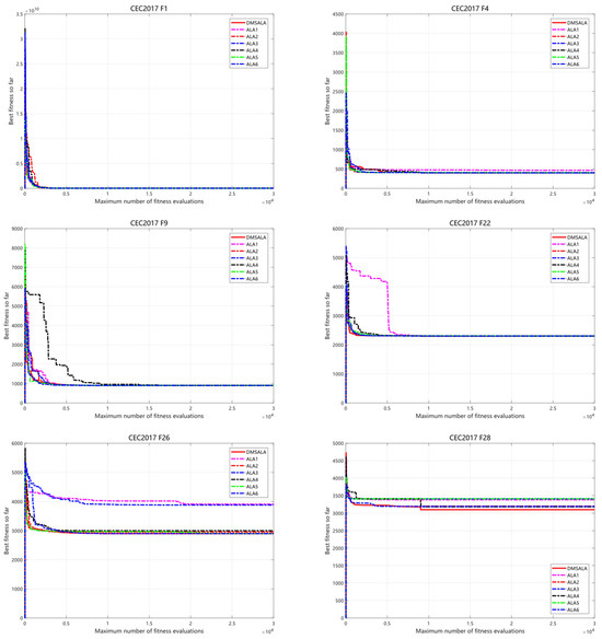
Figure 4.
Convergence curve of DMSALAs and its variants on IEEE CEC 2017.
4.2. Comparison Experiment on IEEE CEC2017
To thoroughly evaluate the optimization performance of the proposed DMSALAs algorithm, we performed comprehensive experiments on the IEEE CECs 2017 benchmark. DMSALAs were compared with eight MHs algorithms, including (ALAs) [22], WMAs [30], PSOs [31], SFOAs [32], BKAs [33], GOOSEs [34], BWOs [35], and GWOs [10], selected for their diverse search mechanisms and proven effectiveness in optimization tasks.
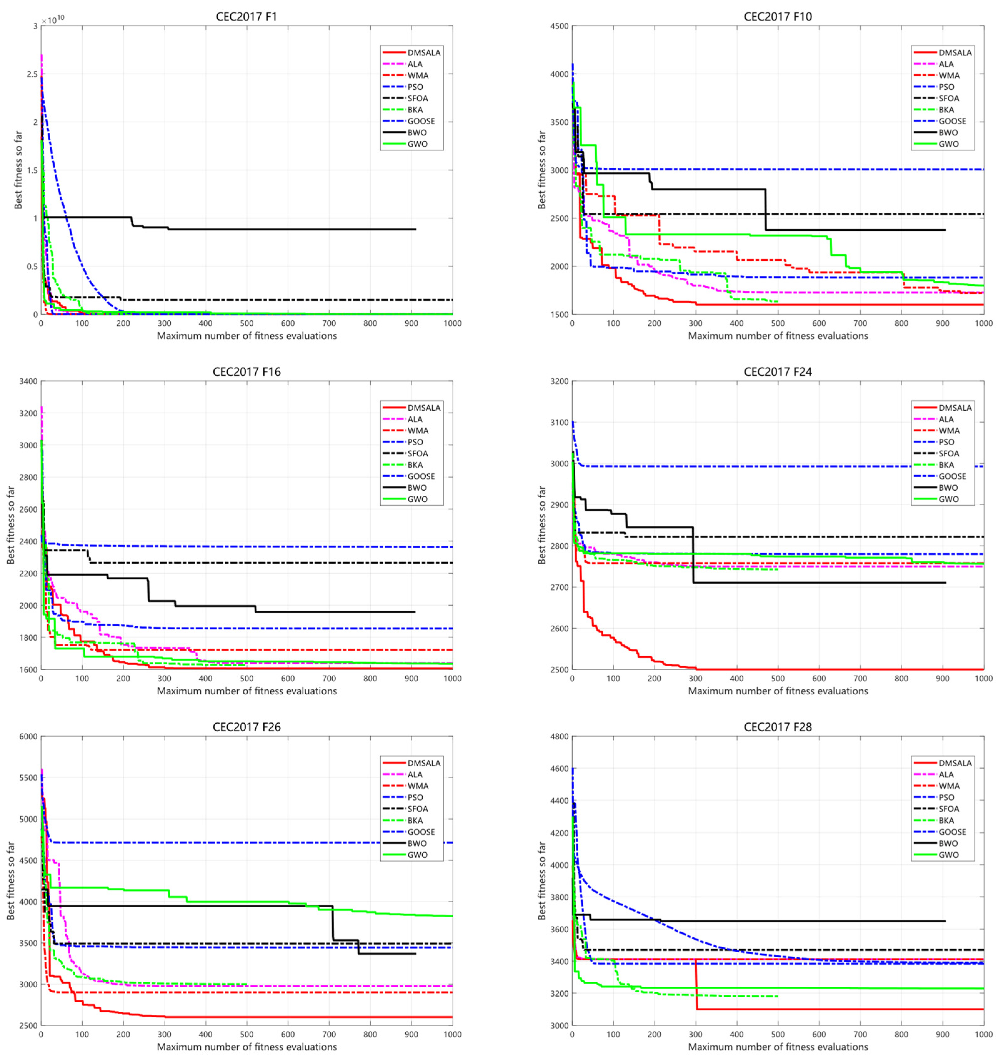
As illustrated in Table 4, the results of the Lilliefors normality test are as follows: a total of 261 tests (29 test functions and nine algorithms), with 48 cases where the normal distribution cannot be rejected and 213 cases of non-normal distribution. These results confirm that our data indeed have significant non-parametric characteristics, thereby providing a sufficient statistical basis for the application of the Friedman test. The DMSALAs successfully pinpointed 21 out of 29 optimal solutions, with a (+/−/=) statistical result of (21/0/8). Its Friedman mean score stands at 1.66, securing the top rank and significantly outperforming all comparative algorithms. ALAs achieved 12 optimal solutions, which confirms that the improvements, including dynamic adaptation mechanisms, hybrid Nelder–Mead integration, and perturbation strategies, have notably enhanced its performance. The (+/−/=) statistic is (12/0/17), accompanied by a Friedman mean of 2.03, ranking second. WMA obtained eight optimal solutions, demonstrating competitive yet less consistent results. Its (+/−/=) statistic is (8/0/21), with a Friedman mean of 3.07, placing it third. BKA identified two optimal values, yielding a (+/−/=) statistic of (2/0/27) and a Friedman mean of 3.52 (fourth place). PSOs secured three optimal solutions, with corresponding metrics of (3/0/26) and 3.86 (fifth place). GWOs only achieved one optimal value, reflecting its limitations in handling complex or high-dimensional problem spaces, with a (+/−/=) statistic of (1/0/28) and a Friedman mean of 4.21 (sixth place). Notably, BWOs, SFOAs, and GOOSEs failed to converge to any global optima, indicating inherent weaknesses in balancing exploration and exploitation. These findings, as visualized in Figure 5, unequivocally validate the dominant performance of the DMSALAs algorithm across evaluated benchmarks.
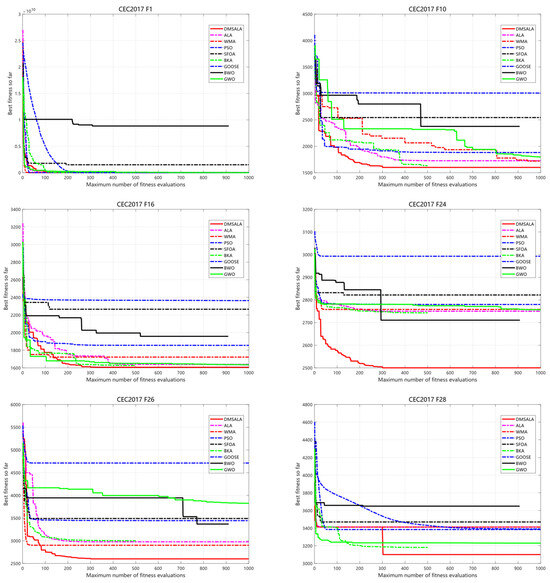
Figure 5.
Convergence curve of DMSALAs and 8 advanced algorithms on IEEE CEC 2017.
4.3. Comparison Experiment on IEEE CEC2022
To evaluate DMSALAs performance on the test set, we contrasted it with the eight previously mentioned algorithms using the IEEE CEC 2022 benchmarking framework. The experimental findings are documented in Table 5, while the convergence trajectories of each algorithm across various test functions are illustrated in Figure 6.
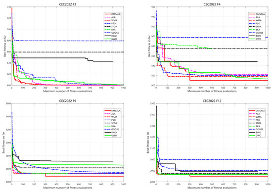
Figure 6.
Convergence curve of DMSALAs and 8 advanced algorithms on IEEE CEC 2022.
As presented in Table 5, the results of the Lilliefors normality test are as follows: a total of 108 tests (12 test functions and nine algorithms), with 21 cases where the normal distribution cannot be rejected and 87 cases of non-normal distribution. These results confirm that our data indeed have significant non-parametric characteristics, thereby providing a sufficient statistical basis for the application of the Friedman test. The DMSALAs successfully obtained 10 out of 12 optimal solutions, with a (+/−/=) statistical result of (10/0/2) and a Friedman mean of 1.42, ranking first and significantly outperforming all competing algorithms. ALAs secured seven optimal solutions, verifying that improvements such as dynamic adaptation, hybrid Nelder–Mead integration, and perturbation strategies effectively enhance its performance. With a (+/−/=) statistic of (7/0/5) and a Friedman mean of 1.58, it ranks second. WMAs achieved five optimal solutions, showing competitive yet less stable performance, with a (+/−/=) statistic of (5/0/7) and a Friedman mean of 2.42, ranking third. Both PSOs and GWOs identified only 2 optimal values, sharing a (+/−/=) statistical result of (2/0/10) with Friedman means of 3.08 and 3.50, ranking fourth and sixth, respectively, which reflects their limitations in handling complex high-dimensional problems. BKAs obtained three optimal values, with a (+/−/=) statistic of (3/0/9) and a Friedman mean of 3.17, ranking fifth. Notably, BWOs, SFOAs, and GOOSEs failed to converge to any global optima, indicating flaws in their exploration–exploitation balance mechanisms.
4.4. Wilcoxon Rank Sum Test
The Wilcoxon rank sum test is employed to assess the disparity between DMSALAs and competitor methods. A significance level of 0.05 is set, and (+|=|−) denotes superiority, equality, or inferiority of the DMSALAs algorithm compared to its competitors. Table 6 illustrates the notable variances found in the majority of functions between our suggested DMSALAs and alternative algorithms. The results are as follows: 182/0/50 and 84/0/12. These results collectively indicate that our proposed DMSALAs exhibit substantial distinctions when compared with the other ten algorithms.

Table 6.
Wilcoxon rank sum test statistical results.
5. Path Planning Problem for Mobile Robots
In this section, we conducted a comprehensive performance evaluation of the DMSALAs algorithm, validating its efficacy in solving the mobile robot path planning problem through comparative analyses with eight benchmark algorithms. The validation was performed across two distinct environments: a simulated testing scenario and the physical operational setting of the RIA-E100 robotic system.
5.1. Simulation Experiment for Mobile Robot Path Planning
To comprehensively evaluate the performance and scalability of the proposed algorithm, experiments were conducted on four grid maps of different sizes: 10 × 10, 20 × 20, 30 × 30, and 40 × 40. This size sequence establishes a uniformly increasing gradient of search space complexity, aiming to systematically assess the algorithm’s adaptability from simple to complex scenarios. The smaller-scale maps are used to verify the basic correctness of the algorithm, while the medium- and large-scale maps are employed to evaluate its convergence behavior, solution quality, and computational efficiency as the problem size increases—thereby assessing the algorithm’s scalability. The evaluated algorithmic parameters consisted of the optimal, average, and standard deviation values of the path length, calculated over 30 independent trials.
The path length in the mobile robot path planning problem is defined as:
where represents the generated route, and represent the number of rows and columns in the map, respectively, and indicates the number of obstacles encountered along the path. First, a smooth path is generated through a midpoint neighborhood search followed by two smoothing processes. Subsequently, the total path length, denoted as , is computed by summing the Euclidean distances between each pair of adjacent points along the trajectory.
The DMSALAs algorithms performance evaluation was executed using MATLAB 2023b software. Simulations were run on a desktop system featuring Windows 11 Pro, an Intel(R) Core (TM) i9-14900KF processor (3.20 GHz), and 128 GB of RAM (Hangzhou China).
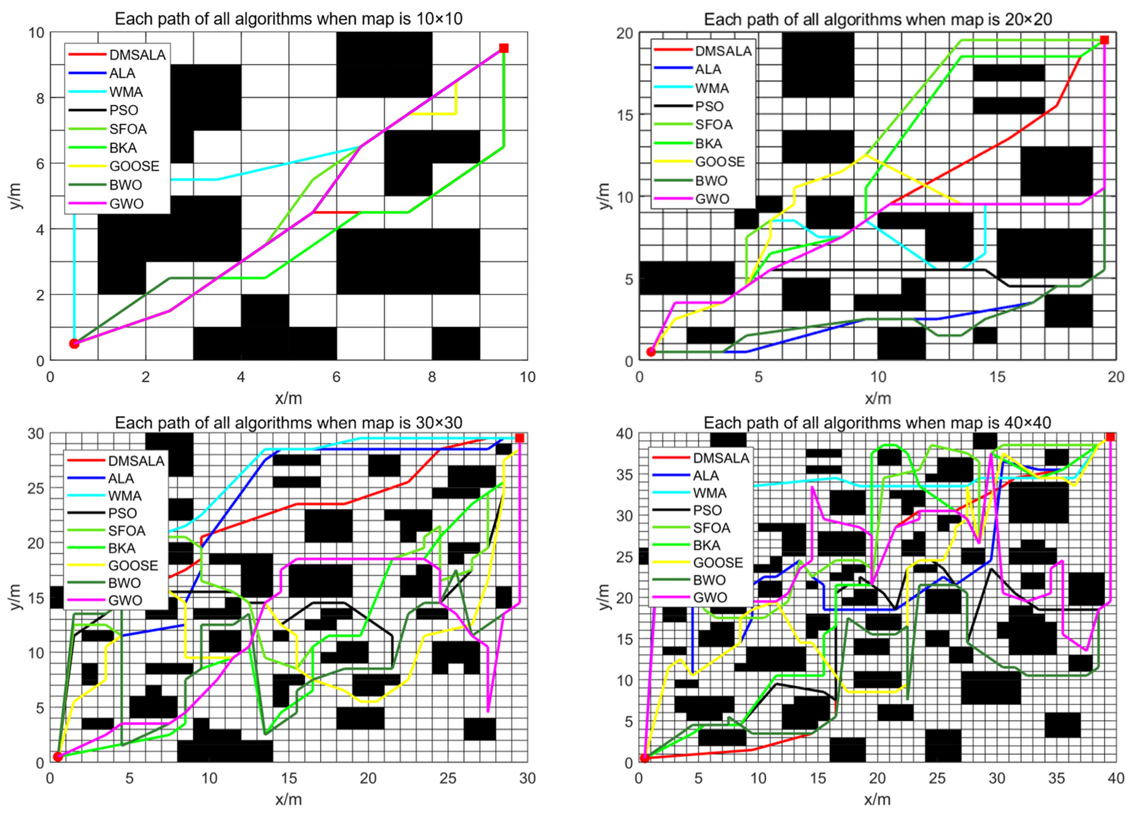
As depicted in Table 7 and Figure 7, the DMSALAs algorithm efficiently located optimal values across four maps with distinct scales and attained the optimal average performance. The Friedman test ranking is the first. Thereby highlighting its superior optimization capability. While DMSALAs demonstrated stable performance, they did not yield the lowest standard deviation in all cases. Notably, the BKA algorithm achieved the best standard deviation in two scenarios, whereas the BWO and WMA algorithms each excelled in one case. This suggests that the DMSALAs algorithm has room for stability improvement.

Table 7.
DMSALAs performance compared with 8 advanced algorithms on 4 different maps.
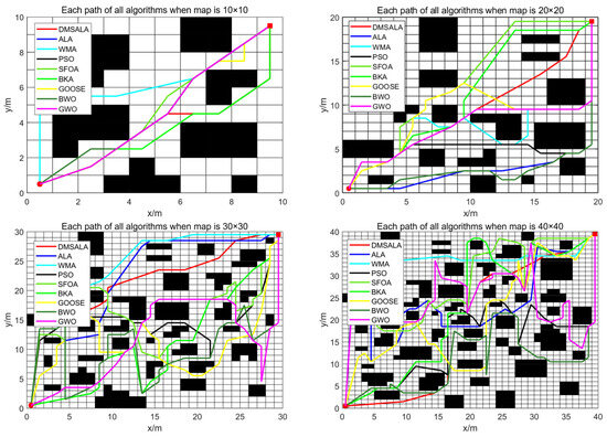
Figure 7.
Path found of DMSALAs and 8 advanced algorithms.
DMSALAs consistently achieved the minimum path lengths (optimal values) across all four map scenarios, demonstrating their superior equilibrium between exploration and exploitation capabilities. The algorithm also exhibited the lowest mean path length across multiple runs, underscoring its robust performance. Although DMSALAs standard deviations remained stable, they were not optimal in all cases (BKAs outperformed in 2 of 4 maps). This minor variability in performance is likely attributed to random perturbations in complex mapping environments. By contrast, BKAs and BWOs occasionally demonstrated better standard deviations, primarily due to their exploitation-oriented strategies. DMSALAs adaptive mechanism prioritizes optimality over strict repeatability, which explains its slightly higher variance trade-off that emphasizes solution quality over absolute consistency.
5.2. Real-World Experimental Verification of DMSALAs for Mobile Robot Path Planning
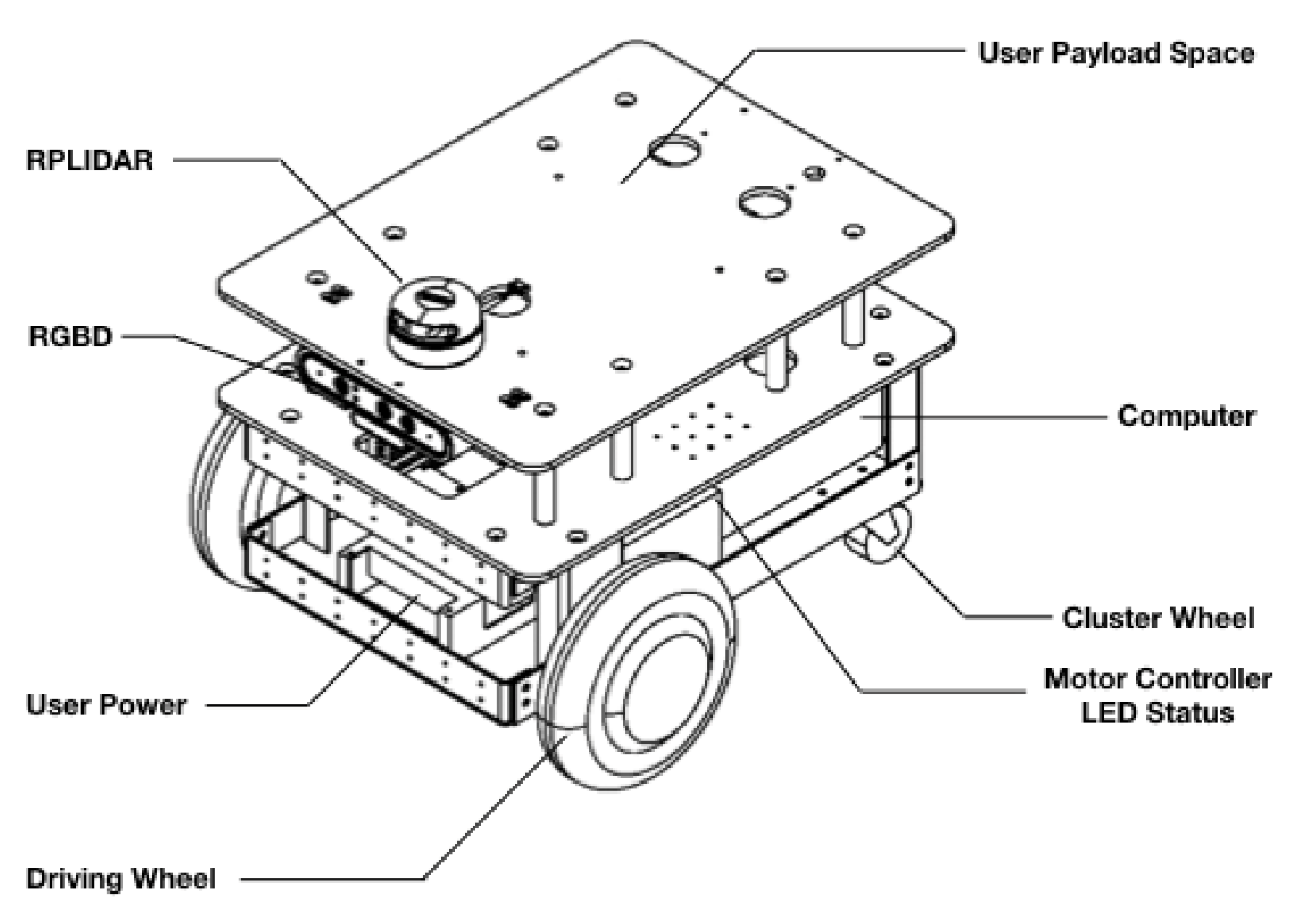
In this section, the DMSALAs algorithm and the eight previously introduced algorithms were experimentally evaluated on the RIA-E100 mobile robot, a compact modular model from GaiTech Robotics’ RIAs series. As illustrated in Figure 8, the robot features a differential-drive configuration with two powered wheels at the front and two passive omnidirectional wheels at the rear, ensuring agile maneuverability. Its computational capabilities are supported by an Intel i5 processor, 8GB of RAM, and a 120GB SSD, enabling real-time data processing. The experimental setup integrates an Astra Orbbec RGBD camera, an Inertial Measurement Unit (IMU), and a 2D LiDAR sensor, facilitating environmental perception. Wireless communication between the control computer and the robot is established via Wi-Fi, ensuring seamless data transfer. The testing environment has a length of 3.2 m and a width of 2.7 m, with obstacles randomly distributed within the area.

Figure 8.
Structural Diagram of the RIA-E100 Mobile Robot.
In Figure 9 and Figure 10, the starting point of the map is located at the lower left corner in the actual map scenario, while the endpoint is positioned at the upper right corner. In contrast, within the Rviz environment, the map starts at the lower right corner and ends at the upper left corner. Cuboid-shaped obstacles are strategically placed to simulate challenging navigation scenarios, with the unobstructed zones designated as navigable regions. To ensure comparability, identical start and end coordinates were assigned across all algorithms. Each algorithm underwent 30 independent runs, during which the minimum path length was recorded. Subsequently, the arithmetic means and variance of these 30 trials were computed to analyze the algorithms’ performance stability statistically. Figure 9 captures the robot’s navigation process in the physical environment, and Figure 10 illustrates the corresponding occupancy grid map generated in Rviz, providing a comprehensive view of the experimental outcomes.

Figure 9.
The operation of the RIA-E100 mobile robot in the real environment.

Figure 10.
Map of the RIA-E100 mobile robot in Rviz.
Table 8 presents the optimal values, mean values, and variances of path lengths derived from 30 independent runs of the DMSALAs algorithm and eight comparative algorithms. DMSALAs attained an optimal path length of 3.687 m and a mean path length of 3.881 m, both of which ranked top-ranked across all algorithms. Although the standard deviation of DMSALAs over 30 runs was not the minimum, standing in third place, trailing only the WMAs and ALAs algorithms, it still maintained a relatively low magnitude. These findings firmly validate the effectiveness of the DMSALAs algorithm in addressing mobile robot path planning challenges.

Table 8.
Results of the DMSALAs and 8 advanced algorithms on the RIA-E100 robot.
6. Conclusions
By integrating a dynamic adaptive mechanism, a hybrid Nelder–Mead method, and a small-range perturbation strategy into the ALAs algorithm, we developed the DMSALAs algorithm. To assess its efficacy, DMSALAs were first compared with six variant algorithms to validate the proposed strategies, then benchmarked against eight advanced algorithms to demonstrate its superior performance. These enhancements effectively address the original algorithm’s core limitations-fixed parameters, weak local search capability, and insufficient diversity preservation-making it better suited for complex optimization tasks. Specifically, the hybrid Nelder–Mead component plays a pivotal role in refining waypoints, minimizing detours, and ensuring smooth trajectories; the dynamic search radius adjustment prevents premature stagnation, and perturbation strategies enable escape from concave obstacle regions.
To further verify DMSALAs applicability in mobile robot path planning, we systematically executed simulation experiments for the DMSALAs algorithm and eight comparative algorithms across four maps with varying scales. Subsequently, we carried out real-world experiments utilizing the RIA-E100 mobile robot within a custom-constructed physical environment. Our dual-approach experimental design, which combines virtual simulations across four maps of varying scales and real-world validations using the RIA-E100 robot, enabled a comprehensive evaluation of the DMSALAs algorithm and eight comparative algorithms. This methodology demonstrated DMSALAs superiority in addressing practical challenges, proving it to be a highly effective optimizer, especially for complex, high-dimensional problems. Its consistent top performance across diverse scenarios highlights its broad applicability in real-world engineering optimizations, such as robotic path planning tasks that demand both solution precision and reliability.
Notably, while DMSALAs demonstrate strong effectiveness, its standard deviation results across various tests indicate room for stability improvements, even after the implemented enhancements. This presents a key direction for future research. Additionally, as this study tested DMSALAs up to 30D problems, exploring its performance in higher-dimensional scenarios (50D and 100D) constitutes another critical research avenue. While this work focuses on mobile robot path planning, future efforts will aim to extend DMSALAs to other practical domains, including industrial robotics and search-and-rescue operations. In this study, high-performance algorithms were not included in the comparative analysis; however, performance comparisons with a broader selection of state-of-the-art algorithms will be conducted in future work and will constitute an important research direction. Furthermore, we plan to carry out rigorous ablation studies to precisely quantify the synergistic effects of the hybrid strategy. Specifically, on the CECs benchmark suite, incremental variants of the algorithm will be compared to disentangle the contribution of the enhanced local search component from the effect of increased function evaluations, thereby providing empirical support for the proposed synergy.
Although current stability and scalability limitations require further investigation, DMSALAs consistent excellence in both benchmark functions and applied path planning solidifies its status as a state-of-the-art optimization tool. Future research will prioritize bridging the gap between theoretical optimization and real-world deployment, ensuring robust performance in dynamic and uncertain environments.
Author Contributions
P.Q.: Conceptualization, Methodology, Writing, Data testing, Reviewing, Software; X.S.: Conceptualization, Funding; Z.Z.: Supervision, Reviewing. All authors have read and agreed to the published version of the manuscript.
Funding
This research was funded by the National Natural Science Foundation of China (No. 52065010 and No. 52165063). The Key Laboratory of New Power System Operation Control of Guizhou Province (Qiankehe Platform ZSYS[2025]007).
Data Availability Statement
The original contributions presented in this study are included in the article. Further inquiries can be directed to the corresponding author.
Conflicts of Interest
The authors declare no conflicts of interest.
References
- Qu, P.J.; Yuan, Q.N.; Du, F.L.; Gao, Q.Y. An improved manta ray foraging optimization algorithm. Sci. Rep. 2024, 14, 10301. [Google Scholar] [CrossRef]
- Xiao, Y.N.; Sun, X.; Guo, Y.L.; Li, S.P.; Zhang, Y.P.; Wang, Y.W. An Improved Gorilla Troops Optimizer Based on Lens Opposition-Based Learning and Adaptive β-Hill Climbing for Global Optimization. Cmes-Comput. Model. Eng. Sci. 2022, 131, 815–850. [Google Scholar] [CrossRef]
- MiarNaeimi, F.; Azizyan, G.; Rashki, M. Horse herd optimization algorithm: A nature-inspired algorithm for high-dimensional optimization problems. Knowl.-Based Syst. 2021, 213, 106711. [Google Scholar] [CrossRef]
- El-kenawy, E.M.; Khodadadi, N.; Mirjalili, S.; Abdelhamid, A.A.; Eid, M.M.; Ibrahim, A. Greylag Goose Optimization: Nature-inspired optimization algorithm. Expert Syst. Appl. 2024, 238, 122147. [Google Scholar] [CrossRef]
- Zhu, F.F.; Shuai, Z.H.; Lu, Y.R.; Su, H.H.; Yu, R.W.; Li, X.; Zhao, Q.; Shuai, J.W. oBABC: A one-dimensional binary artificial bee colony algorithm for binary optimization. Swarm Evol. Comput. 2024, 87, 10156. [Google Scholar] [CrossRef]
- Ebeed, M.; Abdelmotaleb, M.A.; Khan, N.H.; Jamal, R.; Kamel, S.; Hussien, A.G.; Zawbaa, H.M.; Jurado, F.; Sayed, K. A Modified Artificial Hummingbird Algorithm for solving optimal power flow problem in power systems. Energy Rep. 2024, 11, 982–1005. [Google Scholar] [CrossRef]
- Mirjalili, S.; Lewis, A. The Whale Optimization Algorithm. Adv. Eng. Softw. 2016, 95, 51–67. [Google Scholar] [CrossRef]
- Belge, E.; Altan, A.; Hacioglu, R. Metaheuristic Optimization-Based Path Planning and Tracking of Quadcopter for Payload Hold-Release Mission. Electronics 2022, 11, 1208. [Google Scholar] [CrossRef]
- Li, W.Y.; Shi, R.H.; Dong, J. Harris hawks optimizer based on the novice protection tournament for numerical and engineering optimization problems. Appl. Intell. 2023, 53, 6133–6158. [Google Scholar] [CrossRef]
- Mirjalili, S.; Mirjalili, S.M.; Lewis, A. Grey Wolf Optimizer. Adv. Eng. Softw. 2014, 69, 46–61. [Google Scholar] [CrossRef]
- Shao, S.K.; Peng, Y.; He, C.L.; Du, Y. Efficient path planning for UAV formation via comprehensively improved particle swarm optimization. Isa Trans. 2020, 97, 415–430. [Google Scholar] [CrossRef]
- Miao, C.W.; Chen, G.Z.; Yan, C.L.; Wu, Y.Y. Path planning optimization of indoor mobile robot based on adaptive ant colony algorithm. Comput. Ind. Eng. 2021, 156, 107230. [Google Scholar] [CrossRef]
- Mafarja, M.M.; Mirjalili, S. Hybrid Whale Optimization Algorithm with simulated annealing for feature selection. Neurocomputing 2017, 260, 302–312. [Google Scholar] [CrossRef]
- Yu, H.L.; Gao, Y.L.; Wang, L.; Meng, J.T. A Hybrid Particle Swarm Optimization Algorithm Enhanced with Nonlinear Inertial Weight and Gaussian Mutation for Job Shop Scheduling Problems. Mathematics 2020, 8, 1355. [Google Scholar] [CrossRef]
- Li, C.L.; Sun, G.J.; Deng, L.B.; Qiao, L.Y.; Yang, G.Q. A population state evaluation-based improvement framework for differential evolution. Inf. Sci. 2023, 629, 15–38. [Google Scholar] [CrossRef]
- Xiao, Y.N.; Cui, H.; Hussien, A.G.; Hashim, F.A. MSAO: A multi-strategy boosted snow ablation optimizer for global optimization and real-world engineering applications. Adv. Eng. Inform. 2024, 61, 102464. [Google Scholar] [CrossRef]
- Gandomi, A.H. Interior search algorithm (ISA): A novel approach for global optimization. Isa Trans. 2014, 53, 1168–1183. [Google Scholar] [CrossRef]
- Shayanfar, H.; Gharehchopogh, F.S. Farmland fertility: A new metaheuristic algorithm for solving continuous optimization problems. Appl. Soft Comput. 2018, 71, 728–746. [Google Scholar] [CrossRef]
- Padash, A.; Sandev, T.; Kantz, H.; Metzler, R.; Chechkin, A. Asymmetric Levy Flights Are More Efficient in Random Search. Fractal Fract. 2022, 6, 260. [Google Scholar] [CrossRef]
- Pavlik, J.A.; Sewell, E.C.; Jacobson, S.H. Two new bidirectional search algorithms. Comput. Optim. Appl. 2021, 80, 377–409. [Google Scholar] [CrossRef]
- Xu, Y.H.; Zhou, W.N.; Fang, J.A.; Sun, W. Adaptive lag synchronization and parameters adaptive lag identification of chaotic systems. Phys. Lett. A 2010, 374, 3441–3446. [Google Scholar] [CrossRef]
- Xiao, Y.N.; Cui, H.; Abu Khurma, R.; Castillo, P.A. Artificial lemming algorithm: A novel bionic meta-heuristic technique for solving real-world engineering optimization problems. Artif. Intell. Rev. 2025, 58, 84. [Google Scholar] [CrossRef]
- Wei, Q.L.; Liu, D.R.; Lin, H.Q. Value Iteration Adaptive Dynamic Programming for Optimal Control of Discrete-Time Nonlinear Systems. IEEE Trans. Cybern. 2016, 46, 840–853. [Google Scholar] [CrossRef] [PubMed]
- Zhao, Y.W.; Niu, B.; Zong, G.D.; Xu, N.; Ahmad, A.M. Event-triggered optimal decentralized control for stochastic interconnected nonlinear systems via adaptive dynamic programming. Neurocomputing 2023, 539, 126163. [Google Scholar] [CrossRef]
- Liang, H.J.; Liu, G.L.; Zhang, H.G.; Huang, T.W. Neural-Network-Based Event-Triggered Adaptive Control of Nonaffine Nonlinear Multiagent Systems with Dynamic Uncertainties. IEEE Trans. Neural Netw. Learn. Syst. 2021, 32, 2239–2250. [Google Scholar] [CrossRef]
- Mai, C.L.; Zhang, L.X.; Chao, X.W.; Hu, X.; Wei, X.Z.; Li, J. A novel MPPT technology based on dung beetle optimization algorithm for PV systems under complex partial shade conditions. Sci. Rep. 2024, 14, 6471. [Google Scholar] [CrossRef]
- Yin, Z.Y.; Jin, Y.F.; Shen, J.S.; Hicher, P.Y. Optimization techniques for identifying soil parameters in geotechnical engineering: Comparative study and enhancement. Int. J. Numer. Anal. Methods Geomech. 2018, 42, 70–94. [Google Scholar] [CrossRef]
- Ali, A.F.; Tawhid, M.A. A hybrid cuckoo search algorithm with Nelder Mead method for solving global optimization problems. Springerplus 2016, 5, 473. [Google Scholar] [CrossRef]
- Huang, J.; Biggs, J.D.; Bai, Y.L.; Cui, N.G. Integrated guidance and control for solar sail station-keeping with optical degradation. Adv. Space Res. 2021, 67, 2823–2833. [Google Scholar] [CrossRef]
- He, J.H.; Zhao, S.J.; Ding, J.Y.; Wang, Y.M. Mirage search optimization: Application to path planning and engineering design problems. Adv. Eng. Softw. 2025, 203, 103883. [Google Scholar] [CrossRef]
- Kennedy, J.; Eberhart, R. Particle swarm optimization. In Proceedings of the ICNN’95-International Conference on Neural Networks, Perth, Australia, 27 November–1 December 1995; Volume 4, pp. 1942–1948. [Google Scholar] [CrossRef]
- Jia, H.M.; Zhou, X.L.; Zhang, J.R.; Mirjalili, S. Superb Fairy-wren Optimization Algorithm: A novel metaheuristic algorithm for solving feature selection problems. Clust. Comput.-J. Netw. Softw. Tools Appl. 2025, 28, 246. [Google Scholar] [CrossRef]
- Wang, J.; Wang, W.C.; Hu, X.X.; Qiu, L.; Zang, H.F. Black-winged kite algorithm: A nature-inspired meta-heuristic for solving benchmark functions and engineering problems. Artif. Intell. Rev. 2024, 57, 98. [Google Scholar] [CrossRef]
- Hamad, R.K.; Rashid, T.A. GOOSE algorithm: A powerful optimization tool for real-world engineering challenges and beyond. Evol. Syst. 2024, 15, 1249–1274. [Google Scholar] [CrossRef]
- Zhong, C.T.; Li, G.; Meng, Z. Beluga whale optimization: A novel nature-inspired metaheuristic algorithm. Knowl.-Based Syst. 2022, 251, 109215. [Google Scholar] [CrossRef]
Disclaimer/Publisher’s Note: The statements, opinions and data contained in all publications are solely those of the individual author(s) and contributor(s) and not of MDPI and/or the editor(s). MDPI and/or the editor(s) disclaim responsibility for any injury to people or property resulting from any ideas, methods, instructions or products referred to in the content. |
© 2025 by the authors. Licensee MDPI, Basel, Switzerland. This article is an open access article distributed under the terms and conditions of the Creative Commons Attribution (CC BY) license (https://creativecommons.org/licenses/by/4.0/).


