Abstract
This paper investigates a new class of two-dimensional fuzzy difference equations that integrate logarithmic nonlinearities with interaction effects between system variables. Motivated by the need to model complex dynamical systems influenced by uncertainty and interdependencies, we propose a system that extends existing one-dimensional models to capture more realistic interactions within a discrete-time framework. Our approach employs the characterization theory to transform the fuzzy system into an equivalent family of classical difference equations, thereby facilitating a rigorous analysis of the existence, uniqueness, and boundedness of positive solutions. To support the theoretical findings, two numerical examples are provided, illustrating the model’s capacity to capture complex dynamical patterns under fuzzy conditions. An application to a fuzzy population growth model illustrates how the model captures both interaction effects and uncertainty while ensuring well-defined and stable solutions. Numerical simulations show that, for instance, with , , , and , the trajectories of rapidly converge toward a stable fuzzy equilibrium, with uncertainty bands confirming the positivity and boundedness of the solutions.
MSC:
03E72; 39A10; 39A30
1. Introduction
In recent decades, difference equations have emerged not only as mathematical abstractions but also as indispensable tools for understanding and predicting the evolution of dynamical systems across a wide range of fields. From the oscillations of physical systems and feedback loops in engineering to fluctuations in economic indicators and population dynamics in biological models and temporal dependencies in time series analysis (see, for example, [1,2,3,4,5,6]), difference equations offer a powerful framework for capturing the discrete-time evolution of complex phenomena. These equations stand at the crossroads of theory and application, providing essential insights into the qualitative and quantitative behavior of systems that evolve in discrete steps rather than continuously. Their ability to model systems governed by interdependent, time-recursive relationships makes them particularly well suited to both analytical investigations and real-world problem-solving.
In this context, there has been a growing trend in recent years toward moving beyond traditional linear or time-invariant models by introducing generalized formulations such as difference equations with nonlinear dynamics, delay effects, stochastic perturbations, or inherent uncertainties (see, for example, [7,8,9,10]). These advanced models aim to bridge the gap between idealized mathematical representations and the often-unpredictable behavior of real-world systems, thereby offering a richer and more accurate understanding of complex dynamical phenomena.
In recent years, fuzzy set theory has emerged as a significant and versatile extension in the study of difference equations, offering a flexible and realistic framework for modeling uncertainty and vagueness inherent in real-world systems, often beyond the reach of traditional probabilistic approaches. Unlike probabilistic models, which depend on precise statistical data to estimate distributions and characterize randomness, fuzzy models capture uncertain or incomplete information through fuzzy numbers and linguistic variables. This makes them particularly suitable for analyzing phenomena marked by ambiguity or situations in which statistical control is impractical. This capability has empowered researchers to tackle problems involving systems with poorly defined parameters or those influenced by human judgment and subjective assessments, which often resist strict quantitative analysis. As a result, fuzzy difference equations have gained increasing recognition as effective tools for exploring the dynamics of systems affected by structural or environmental uncertainty, especially in fields such as economics, mathematical biology, population dynamics, the social sciences, and ecosystem management. The intersection between discrete-time modeling and uncertainty has given rise to new research directions focused on examining the qualitative properties of fuzzy difference equations, including existence, uniqueness, stability, attractivity, and long-term behavior. These studies have contributed to the development of models that are better equipped to reflect complex realities and adapt to changing conditions. It is also noteworthy that the role of fuzzy difference equations extends beyond theoretical analysis; they have become central to the advancement of computational methods and numerical simulations in real-world systems, thereby opening broad avenues for interdisciplinary research and practical applications.
The recent literature has increasingly focused on the analysis of nonlinear fuzzy difference equations, owing to the mathematical and conceptual challenges they present in addressing the inherent imprecision and uncertainty of real-world data and models. In response, various methodologies and theoretical frameworks have been proposed to tackle these challenges while striving to balance modeling realism with mathematical tractability. Among the most prominent approaches (see, for example, [11,12]) is the Zadeh’s extension principle, which enables the extension of classical mathematical operations to fuzzy contexts by generalizing functions and operations defined on real numbers to fuzzy numbers across -cut levels. While this principle offers notable flexibility and ease of application, it may sometimes yield solutions with excessively broad fuzzy supports. This expansion of the solution set can amplify uncertainty, particularly when dealing with nonlinear systems or structurally complex equations. As a more conservative alternative, Stefani’s g-partition method has emerged as a promising approach for controlling the spread of fuzzy support. By applying constrained operations, this method helps ensure that solution ranges remain within acceptable bounds. It has proven particularly effective in the study of nonlinear equations, as it facilitates the derivation of more compact and reliable solutions while reducing the uncertainty often associated with the traditional Zadeh’s extension principle. Although the g-partition method does not yet enjoy the same level of generality or widespread adoption as the Zadeh’s extension principle, recent studies have highlighted its capacity to address a broad spectrum of applications, positioning it as a compelling option for the precise analysis of fuzzy dynamical systems. As a result, the trade-off between these two methodologies has become a central theme in contemporary research, especially for scholars seeking to strike a balance between solution precision and analytical flexibility in the fuzzy modeling of nonlinear systems.
Fuzzy difference equation models represent a promising approach for describing the behavior of realistic, nonlinear, and complex systems, particularly due to their natural and flexible capacity to account for uncertainty in both data and model structures. This field has seen notable advancements, starting with a focus on one-dimensional fuzzy difference equations, especially those of the Riccati type, which have been extensively analyzed in numerous studies, including the works of [13,14,15]. Representative examples of such models include the following one-dimensional equation:
whose key properties, including existence, uniqueness, stability, and asymptotic behavior, have been thoroughly investigated. The work of Usman et al. [16] further advanced this research direction by analyzing a logarithmic fuzzy difference Equation (1). They demonstrated that Equation (1) admits a non-negative solution and possesses an equilibrium point, and they explored its stability and recurrence properties using various analytical techniques such as characterization theory, g-partitioning, the variational iteration method, and mathematical inequalities. More recent studies have shifted toward two-dimensional models with special structures, emphasizing systems that involve mutual interactions between variables. For instance, Althagafi and Ghezal [17] examined the following system:
Attia and Ghezal [18] extended the analysis of fuzzy difference equations from one-dimensional to two-dimensional cases by studying the following system:
Their study focused on comparing the qualitative behavior of two-dimensional systems with their one-dimensional counterparts. In a subsequent work, Althagafi and Ghezal [19] proposed an extended system that incorporates the following multiple delay effects:
They provided a rigorous analysis of the existence, boundedness, and stability of solutions, along with numerical studies that demonstrated the applicability of these systems in fuzzy modeling. In the context of analyzing population and community models under fuzzy conditions, recent studies [20,21,22] have established fuzzy difference equations as a fundamental tool for understanding the dynamics of systems characterized by imprecise data and complex interactions.
While the aforementioned studies [16,17,18] have significantly contributed to the development of fuzzy difference equations, they remain limited to either one-dimensional frameworks or two-dimensional systems that do not explicitly include logarithmic interactions between variables. In contrast, the present study introduces a new two-dimensional fuzzy difference system that incorporates both fuzzy uncertainty and logarithmic coupling effects between components. This formulation not only extends the classical logarithmic fuzzy model developed by Usman et al. [16] but also provides a natural generalization that accounts for interactions between variables through doubly coupled coefficients. Usman’s model is thereby transformed into a two-dimensional structure; however, it also differs from the two-dimensional frameworks developed by introducing Althagafi, Ghezal, and Attia [17,18,19] by incorporating a nonlinear logarithmic mechanism governing the interaction between fuzzy variables. Thus, the proposed model offers a new theoretical framework that captures the attenuating interaction effects under uncertainty, an aspect not explicitly addressed in previous research.
Despite the significant research momentum and continuous efforts dedicated to the study of fuzzy difference equations, a notable knowledge gap still persists, particularly regarding the lack of in-depth and systematic investigations of two-dimensional systems with nonlinear structures and interacting components. This gap becomes even more pronounced when considering systems that combine nonlinear features, such as logarithmic processes and transformations involving fractional powers of fuzzy variables. Such models are essential, as they more accurately represent the complexity and interdependence observed in real-world phenomena. Two-dimensional fuzzy systems involving variable interactions do not merely describe the isolated dynamics of individual variables; rather, they emphasize the effects of mutual interdependence, often giving rise to intricate behaviors, including oscillations, feedback loops, and coupled dynamics. Despite their potential relevance to natural, economic, and biological systems, the mathematical analysis of such models remains relatively limited. There is a clear need for methodological advancements that can simultaneously address both the complexities of fuzziness and nonlinear interdependencies. In response to this research gap, the present paper aims to bridge it by proposing a novel system of two-dimensional fuzzy difference equations that incorporates both logarithmic effects and variable interactions. The system is defined as follows:
where and for all are successive positive fuzzy numbers representing the system’s dynamic variables and A, B, C, , , and are fuzzy parameters. This proposed model not only embeds logarithmic operations within the framework of fuzzy difference equations but also emphasizes the structural role of variable interactions, a combination expected to produce unconventional dynamic behaviors that necessitate rigorous mathematical analysis. Accordingly, this study seeks to make an original contribution to the understanding and analysis of this class of systems, with a particular focus on the properties of existence and uniqueness.
The main motivations behind proposing this new model arise from a combination of scientific and methodological considerations aimed at addressing the existing challenges in analyzing fuzzy difference equations with two-dimensional structures and nonlinear interactions. This research direction is driven by the pressing need for advanced mathematical tools capable of capturing the complex dynamical behavior of systems influenced by uncertainty and mutual interactions. A key aspect of this approach is the incorporation of the mitigating properties of the logarithmic function, which is known for its ability to moderate sharp changes and smooth out large fluctuations. The logarithm thus facilitates more accurate modeling of systems characterized by abrupt variations or sudden perturbations. By integrating this property into fuzzy difference equations, the model seeks to provide a more realistic and relatively stable description of system dynamics over time. Another central component of the methodology is the application of characterization theory to transform the fuzzy system into an equivalent classical system. By employing tools such as the -cut characterization, the original fuzzy system is reformulated as a family of classical equations associated with distinct cut levels. This transformation enables the application of established mathematical analysis techniques while preserving the essential features of the fuzzy solutions. The paper focuses on investigating the existence, uniqueness, and boundedness of positive solutions. Additionally, numerical examples are provided to illustrate and validate the theoretical findings, thereby adding a practical dimension to the analysis. Through this integrated approach, the present paper aims to address a tangible gap in the literature on fuzzy difference equations by exploring a novel line of inquiry that combines rigorous classical methodologies with contemporary tools for analyzing nonlinear fuzzy systems with interacting variables. Moreover, the proposed framework offers a flexible mathematical foundation that can be adapted and extended to meet diverse application needs across various fields, including the natural sciences, engineering, economics, and social sciences, thereby opening new avenues for future research.
The introduction of the logarithmic process into the proposed system originates from numerous real-life phenomena that exhibit the so-called diminishing return effect. In many biological, economic, and social systems, the mutual influence between components is not constant but gradually weakens as the intensity of interaction or system density increases. For example, in population models, the benefits resulting from cooperation or interaction between groups rise sharply at first but then gradually decline as the population size grows or as the system approaches its ecological capacity. The logarithmic function naturally captures this behavior, as it increases rapidly at small values and then levels off at larger ones, making it a suitable mathematical tool for modeling nonlinear effects that decrease over time or with increasing density. From this perspective, the use of the logarithm in the proposed system is not merely a formal choice, but rather reflects a universal real-world principle observed across nature, economics, and society, where mutual influences tend to saturate instead of increasing indefinitely. Beyond the experimental motivation, the adoption of the logarithmic interaction term in the proposed system is also supported by analytical considerations. Mathematically, the logarithmic function is one of the simplest forms that exhibit both monotonicity and concavity, two properties that naturally represent saturation and decreasing sensitivity as interaction intensity increases. Furthermore, the smoothness and differentiability of this function ensure that the resulting system remains mathematically tractable, allowing for a careful examination of its stability and limiting behavior. From an applied perspective, many biological and socio-economic models confirm that growth and interaction rates tend to saturate at high levels, making the logarithmic formulation not only mathematically convenient but also conceptually consistent with realistic behavior under uncertainty.
Main Contributions
The main contributions of this paper can be summarized as follows:
- The introduction of a novel two-dimensional fuzzy difference system that incorporates logarithmic interaction terms, allowing the model to capture diminishing influence effects between interacting components under uncertainty.
- The development of an analytical framework based on the characterization theorem, which transforms the fuzzy system into an equivalent family of crisp difference equations. This transformation enables a rigorous analysis of the existence, uniqueness, and boundedness of positive fuzzy solutions.
- Establishment of theoretical results on positivity, boundedness, and stability, providing sufficient conditions that ensure the proposed fuzzy trajectories remain well-defined and convergent under admissible parameter ranges.
- An extension of existing one-dimensional logarithmic fuzzy models (e.g., Usman et al. [16]) to a bidimensional coupled structure that integrates both cross-interaction and self-limiting effects, thereby distinguishing it from prior works on higher-order or separable fuzzy systems.
- Implementation of numerical simulations confirming the theoretical findings and visualizing the uncertainty propagation through fuzzy parameters, demonstrating convergence to stable fuzzy equilibria.
- An application to fuzzy population dynamics, which demonstrates the model’s practical relevance and illustrates how the logarithmic coupling reproduces realistic behaviors such as saturation and limited growth under environmental uncertainty.
This paper is organized into six main sections. Section 1 provides the introduction, outlining the scientific motivation behind the study and highlighting its primary objectives and key contributions, which are detailed in the subsection on main contributions. Section 2 reviews the fundamental concepts and preliminary results related to fuzzy difference equations, including the preliminary definitions and theoretical tools required for analyzing the proposed system. Section 3 applies the characterization approach to transform the fuzzy system into an equivalent system of classical difference equations and investigates the existence, uniqueness, boundedness, and continuity of positive solutions. Section 4 is devoted to establishing the existence and uniqueness of positive solutions for the proposed system. Section 5 presents the numerical simulations, including illustrative examples that demonstrate the dynamic behavior of the system, such as a fuzzy population growth model with logarithmic interactions. Finally, Section 6 concludes the paper by summarizing the main findings of the study and suggesting potential directions for future research.
2. Basic Definitions and Auxiliary Results
In this section, we establish the theoretical foundations necessary for the analysis presented in the subsequent parts of this study. We begin by revisiting the key definitions and mathematical structures related to fuzzy numbers, their basic operations, and the properties of the associated metric spaces. These fundamental concepts are essential for formulating and analyzing fuzzy difference equations within a rigorous mathematical framework. Additionally, we introduce a set of lemmas and characterization results that serve as essential tools for establishing the main theoretical findings of this paper. For additional details regarding the fuzzy concepts and methodologies employed here, the reader is referred to the works of [23,24,25,26,27,28].
Definition 1.
Let be a function representing the degree of membership of each real number . We say that Z is a fuzzy number if the following four conditions are satisfied:
- (C.0)
- Normality:There exists a real number such that its degree of membership is maximal, that is, .
- (C.1)
- Fuzzy Convexity:For all and the following inequality holds:
- (C.2)
- Upper semi-continuity:The function is upper semi-continuous on ; that is, it does not exhibit sudden upward jumps in its values.
- (C.3)
- Compact support:The set of points with positive membership values , is a compact set, meaning it is both closed and bounded.
Definition 2.
-cut and fundamental functions on fuzzy numbers
Let denote by the space containing all fuzzy numbers defined on . For all and a fuzzy number , the λ-cut of the fuzzy number Z is defined as . The support of the fuzzy number Z, denoted by or , is given by A fuzzy number Z is said to be positive if its support is entirely contained in that is, The set of positive fuzzy numbers is denoted by In the special case where Z is a positive real number (considered as a constant fuzzy number), its λ-cut degenerate and given by , Basic operations on fuzzy numbers via λ-cuts: Let Y and Z be two fuzzy numbers such that , , . Let be a positive real number. Then, the following operations are defined using the concept of λ-cut as follows:
- Addition:The λ-cut of the sum of the two numbers is given by
- Scalar Multiplication:Cut-λ of the number is:
- Multiplicative Inverse:The inverse of the λ-cut of Z is given by .
- Division-g :If exists, there are two states as follows:
- –
- State : If then and
- –
- State : If then and
Furthermore, we define the following sequence associated with the fuzzy environment. Let be a real-valued sequence relevant to the fuzzy system, where each . This sequence may serve either as a determinant of the cut-off levels or as an analytical tool to facilitate the study of the system’s dynamic behavior.
Lemma 1.
Properties of fuzzy interval functions
Let Z be a fuzzy function defined on . For all , suppose that the λ-cut of the fuzzy number Z is given by , where and are real-valued functions satisfying the following properties:
- is a non-decreasing and left-continuous function.
- is a non-increasing and right-continuous function.
- is greater than or equal to .
These properties guarantee that a fuzzy number can be represented at each λ-cut by a real interval whose bounds vary consistently with the confidence level λ: the lower bound is a non-decreasing function, and the upper bound is a non-increasing function. This reflects the natural cumulative structure of fuzzy numbers.
The following lemma provides the characterization of the min and max operations at the -cut for fuzzy numbers.
Remark 1.
In this paper, we adopt the convention commonly used in several works [29,30], where is left-continuous and non-decreasing, while is right-continuous and non-increasing. This convention is practically equivalent to the classical definition, where both functions are taken as left-continuous, and it preserves the nested and consistent structure of the λ-cut representation.
Lemma 2.
Properties of min and max operations on λ-cuts of fuzzy numbers
Let Y and Z be two fuzzy numbers with λ-cuts given by and . Let T be another fuzzy number with λ-cut representation .
Then, if and only if for all and
Similarly, we say that if and only if for all and
Definition 3.
Bounded and persistent sequences of positive fuzzy numbers
A sequence of positive fuzzy numbers is said to be bounded and persistent if the following two conditions are satisfied: there exists and there exist two positive fuzzy numbers such that for all and .
Lemma 3.
Combinatorics of a continuous function with -cut of fuzzy numbers
Let be a continuous function, and let be fuzzy numbers. Then, for all , the following holds:
3. Methodology
The methodological framework employed in this study is summarized in Figure 1. It combines both analytical and computational steps to investigate the proposed two-dimensional fuzzy difference system featuring logarithmic interaction terms.
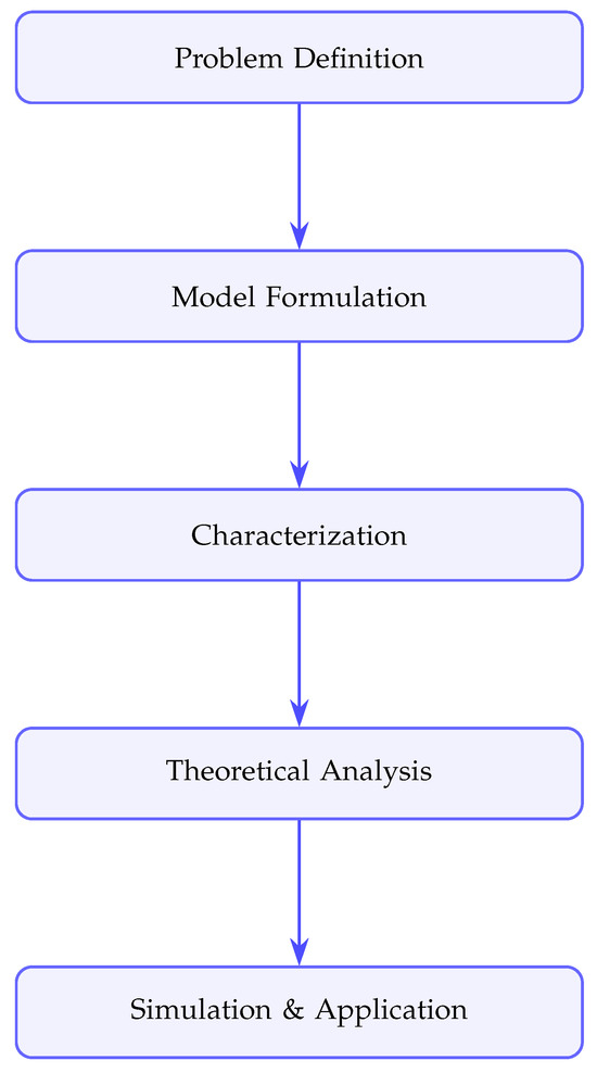
Figure 1.
Flowchart of the methodology used in this paper.
The main stages of the methodology are outlined below:
- Step 1:
- Model formulation. Formulate the proposed two-dimensional fuzzy difference system incorporating logarithmic nonlinearities to capture diminishing interaction effects between system variables.
- Step 2:
- Characterization. Utilize the characterization theorem to transform the fuzzy system into an equivalent family of crisp difference equations for each -cut level.
- Step 3:
- Analytical investigation. Prove the existence, uniqueness, positivity, and boundedness of the fuzzy solution using recursive analysis and inequality techniques.
- Step 4:
- Numerical simulation. Conduct computational experiments to verify theoretical results and explore the dynamical behavior of the system under fuzzy uncertainty.
- Step 5:
- Application. Illustrate the applicability of the proposed model through a fuzzy population growth scenario with interactive effects.
4. Existence, Uniqueness, and Global Stability of the Fuzzy Difference System (2)
In this section, we examine the fuzzy difference system (2), assuming that both the coefficients and the initial conditions are strictly positive fuzzy numbers. We begin by establishing the existence and uniqueness of positive solutions, ensuring that the system’s evolution is well-defined and mathematically consistent for any admissible set of initial conditions. Next, we investigate the boundedness and persistence of these solutions, confirming that they remain within finite, controlled bounds over discrete time and exhibit stable and regular behavior, properties that prevent the system from diverging or collapsing.
The analytical proofs developed in this section are grounded in the classical framework of fuzzy analysis, which relies primarily on -cut representations, monotonicity arguments, and recursive inequalities. Although these methods are standard in the study of fuzzy difference equations, their comprehensive presentation is retained here for the sake of clarity and completeness, particularly since the proposed bidirectional logarithmic coupling introduces nontrivial interdependencies between the fuzzy components.
Before addressing the system’s qualitative dynamics in detail, it is essential to establish the existence and uniqueness of positive fuzzy solutions, as these properties form the theoretical cornerstone for analyzing stability, persistence, and long-term behavior. The following theorem guarantees that, for every admissible set of initial conditions, the system admits a unique and positive fuzzy solution.
Theorem 1.
Proof.
Let the initial conditions , be given as positive fuzzy numbers. We consider the sequence that satisfies the system of fuzzy difference Equations (2). Our goal in this section is to establish the existence and uniqueness of a positive fuzzy solution corresponding to these initial conditions. We first analyze the -cuts representation of the fuzzy components for all . The fuzzy numbers are expressed as follows:
for all Relying on the definitions provided in (3), the structural form of the system (2), and employing the property stated in Lemma 3, we derive the recursive relations governing the evolution of -cuts for all
Applying the properties of fuzzy arithmetic operations on the -cuts, as well as the logarithmic monotonicity over positive intervals, we obtain
for all Hence, according to the system (4), it admits a unique positive solution , provided that the initial conditions for , are given for all . We now assert that the collection for all , and for the prescribed initial conditions, completely characterizes the fuzzy solution of the system (2) associated with the initial conditions and for . In other words, the fuzzy components and are uniquely determined by their -cuts via the following relationships:
Conversely, let us consider the positive fuzzy initial conditions and for , and suppose these generate the -cuts solutions and to the system (2), for all . Assume further that B, C, , , and are positive fuzzy numbers. Then, according to Lemma 1, for any , the cut-interval bounds satisfy
for . We now establish by induction that for all
From (5) and (6), the result clearly holds for . Assuming the hold for all , with , we now examine the state . Using the recursive system (4) together with the inductive hypothesis and applying the monotonicity properties of the involved mappings, we deduce
Hence, (6) is fully verified. Furthermore, invoking both (5) and (6), we obtain
for all Considering that B, C, , , , and for are elements of , it follows that the corresponding -cut bounds, namely and for are all left-continuous functions. Consequently, by direct inspection of (7), we conclude that , , , and are also left-continuous. Applying the principle of mathematical induction, it is straightforward to prove that the sequences , , , and preserve left-continuity for all In order to establish the compactness of the unions and , it suffices to demonstrate that these unions are bounded subsets of . Given the positivity of A, B, C, , , , and for , there exist positive constants , , , , , , , , , , , , , , , , such that
for all for . Substituting into (7), we deduce the bounds
for all , as established in (7). Therefore, the unions , are bounded, hence compact subsets of . By induction, this property extends to every , thereby confirming that the sets , are compact and contained entirely within for all . In conclusion, combining inequality (6), the established compactness, positivity, and left-continuity of the interval bounds, we assert that and define a sequence of positive fuzzy numbers , satisfying system (2) for all and . To demonstrate that the sequence constitutes a solution of system (2) with the initial conditions and for , we recall the explicit expressions for the following -cuts:
for all . This establishes that indeed satisfies system (2) with the prescribed initial conditions and for . To prove the uniqueness of the positive fuzzy solutions, suppose, for contradiction, that there exists another solution of system (2) sharing the same initial conditions and for . By applying the same reasoning to the -cuts, we obtain and for all and . Therefore, and for all and , which implies and for all . This confirms the uniqueness of the positive fuzzy solutions. Finally, if State (b) occurs (i.e., the alternative form of the cut-based representation), the proof proceeds along the same lines by analogous arguments, thus completing the proof. □
To gain a deeper understanding of the qualitative behavior of the positive solutions to system (2), it is essential to investigate two key properties: boundedness and persistence. The boundedness of solutions ensures that the system’s trajectories remain within a finite and controlled range over time, thereby preventing divergence to infinity. Conversely, persistence guarantees that the positive components of the solution do not decay to zero, thereby preserving the system’s long-term dynamical activity and preventing extinction or collapse in the long term. In what follows, we rigorously demonstrate that every positive solution of system (2) exhibits both boundedness and persistence, provided that all parameters and initial conditions are positive fuzzy numbers. This result further reinforces the mathematical soundness and practical relevance of the proposed fuzzy difference model.
Theorem 2.
Proof.
Let be any positive solution of system (2). By examining its equivalent formulation (4), we can derive explicit upper bounds for the -cut components of the solution. Indeed, for all and , the following inequalities hold:
Under , , we can prove by induction that if
where
then for all
On the other hand, using the structure of (4), (9) and for all we obtain
we can write as
where
Therefore, combining the above bounds, we conclude that for all
This double inequality confirms that the positive solution of system (4) is both bounded (above) and persistent (below), which completes the proof of the claimed properties. □
Remark 2.
It is worth noting that the proof proposed in this paper primarily employs the recursive inequalities approach to demonstrate the existence of a unique positive solution to the system. This method offers conceptual simplicity and analytical transparency in tracing the evolution of fuzzy sequences and verifying their confinement within positive and bounded limits. However, this approach is not inherently inconsistent with the contraction mapping principle or the fixed-point framework. Indeed, the given system can be reformulated equivalently, allowing the recursive relation to be interpreted as a contraction operator in a suitable space of fuzzy sequences equipped with an appropriate metric. In this sense, the recursive inequalities utilized here may be viewed as a practical realization of the indirect application of the contraction principle, thereby justifying their use in demonstrating the existence and uniqueness of the solution without the explicit construction of the contraction constant.
5. Numerical Simulations
This section presents numerical simulations of the proposed fuzzy difference system (2). By considering different initial conditions and varying values of the cut-level parameter , the behavior of the system is visualized over discrete time steps. These simulations not only illustrate the boundedness and persistence of the fuzzy solutions but also offer insights into how initial fuzziness and interaction structures affect long-term dynamics.
Example 1.
This example considers the system (2) with fuzzy coefficients A, B, C, , , and are defined as follows:
The initial conditions are represented by fuzzy numbers denoted as , and , respectively,
From (10) and (11), we obtain
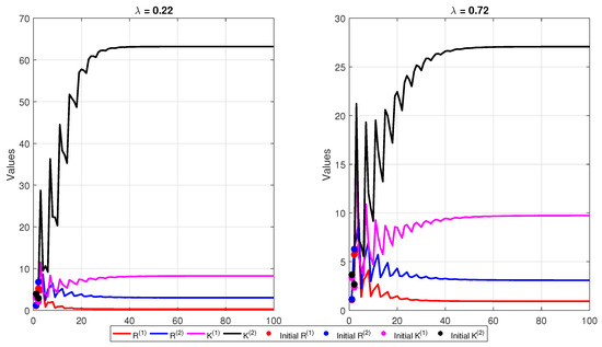
The simulation is performed for two different levels of , representing low- and high-confidence intervals, respectively. The results are displayed in Figure 2, showing the evolution of the left and right endpoints of the fuzzy sequences and
Figure 2.
Time evolution of the fuzzy system (2) for initial conditions in Example 1.
Aspects of the proposed numerical results, the following table provides a summary of the equilibrium values and several accuracy and convergence indices for the studied system at different levels of the membership parameter . This presentation aims to confirm the stability of the numerical solutions and to demonstrate the rate of convergence toward the equilibrium points.
Table 1 shows that, for both values of the membership -cuts, the proposed system converges rapidly toward stable equilibrium points. The residual errors are on the order of , indicating very high numerical precision. The convergence rate and final error are nearly zero, confirming the robustness and stability of the iterative process. Moreover, the equilibrium values vary smoothly with , reflecting the regular and consistent dynamic behavior of the system under different fuzzy conditions.

Table 1.
Quantitative numerical results for different values of the membership -cuts.
To illustrate the numerical relationship between the degree of fuzzy ambiguity and environmental uncertainty in the proposed system, a series of numerical experiments were performed for different values of the fuzzy parameter amplitude . This amplitude represents the level of uncertainty in the system’s basic parameters, where the degree of ambiguity increases as increases. Table 2 presents the resulting equilibrium values , along with the numerical residual value, allowing the direct observation of how the amplitude of ambiguity affects the system’s stability and response.
Table 2.
Effect of fuzzy parameter width () on equilibrium variability.
From Table 2, it is evident that increasing the amplitude of the fuzzy parameter leads to a noticeable change in the equilibrium values of all studied variables. For small values of , the equilibrium values remain nearly stable and convergent, whereas gradual increases in cause these values to diverge and exhibit greater dispersion, particularly for and . This behavior indicates that increasing the degree of ambiguity in the parameters, representing higher environmental uncertainty, is directly reflected in the system’s outputs through larger fluctuations and variations in the equilibrium points. These results therefore provide clear numerical evidence that fuzzy ambiguity amplifies the variability in the system’s dynamic behavior.
Example 2.
This example considers the system (2) with fuzzy coefficients A, B, C, , , and are defined in (10). Here, the initial conditions are represented by fuzzy numbers denoted as , and , respectively,
From (12), we obtain
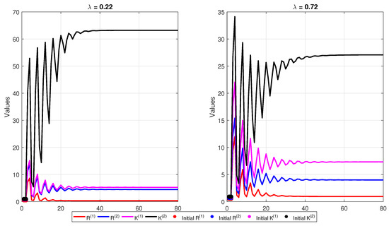
As before, simulations are conducted for . The results are displayed in Figure 3, showing the evolution of the left and right endpoints of the fuzzy sequences and .
Figure 3.
Time evolution of the fuzzy system (2) for initial conditions in Example 2.
The simulation results presented in Figure 2 and Figure 3 clearly confirm the theoretical analysis and reveal several important dynamical features of the proposed fuzzy system. First, both figures exhibit stability and attractor behavior, as the trajectories of and , for all -cuts, converge toward compact and bounded regions. This observation confirms the analytical results regarding global boundedness and persistence of positive fuzzy solutions. Second, the effect of the membership level is evident: smaller -values (e.g., 0.22) generate wider uncertainty bands, indicating higher fuzziness, while larger values (e.g., ) produce narrower bands, corresponding to more precise behavior. Third, comparing the two examples shows that initial fuzziness significantly affects transient dynamics; systems initialized with narrower fuzzy spreads reach equilibrium faster and display smoother trajectories, whereas broader spreads yield more pronounced oscillations before settling down. Finally, the system demonstrates a structural symmetry between and , as both evolve in a coupled and balanced manner throughout the iterations, reflecting the inherent bidirectional interaction embedded in system (2). Overall, the numerical simulations confirm the theoretical predictions and highlight the model’s ability to capture stable, realistic, and uncertainty-aware dynamics in discrete-time fuzzy environments.
Remark 3.
It is important to note that the two-dimensional logarithmic fuzzy system proposed in this work represents a significant generalization of the one-dimensional model developed by Usman et al. (2024), [16]. Both models share the use of logarithmic nonlinearity to represent the diminishing effect. However, the proposed system introduces a bidirectional coupling mechanism between the two principal variables, which enriches the system’s dynamic behavior and more accurately reflects the interactions observed in real-world systems. Numerical simulation results indicate that the system preserves fundamental properties such as positivity, boundedness, and continuity over a wider range of fuzzy parameters than those of the one- dimensional model, demonstrating its numerical robustness and structural stability under uncertainty. The presence of this bidirectional coupling also allows for a more natural transfer of fuzzy ambiguity between system components, providing a more realistic representation of joint influences and complex interactions. When the proposed system is reduced to the special case in which the condition holds, with the selection of symmetric coefficients, the resulting model recovers the basic structure of the Usman et al. [16] model. This demonstrates that the current model is not merely an extension in dimensionality but rather a structured and coherent generalization that preserves the essential properties of the original model while introducing new structural interactions that enrich its dynamics and broaden its potential biological and economic applications.
Remark 4.
It is important to note that the research does not provide an explicit analytical proof for the existence of equilibrium points in the proposed system, mainly due to the complex nature of the logarithmic relationships involved in the model. The inclusion of logarithmic terms within the evolution equations renders the resulting relations highly nonlinear and mixed in order, combining linear and logarithmic components in a complex structure. This complexity prevents the direct analytical derivation of a closed-form expression for the equilibrium points. However, the structural analysis of the system, together with the results of numerical simulations, strongly suggests the existence of a positive and numerically stable equilibrium region toward which the resulting sequences of variables converge over time. This stable numerical behavior implicitly reflects the satisfaction of the existence and positivity properties discussed theoretically in the main body of the research. The dependence of this approximate equilibrium on the fuzzy coefficients has been examined indirectly through the analysis of λ-cuts, where each λ-cut corresponds to an equivalent crisp system that preserves the fundamental properties of the solutions. The variation in the numerical equilibrium position can therefore be interpreted as a smooth and continuous effect arising from the fuzzy coefficients. Changing the degree of membership λ leads to a gradual shift in the equilibrium position without inducing any abrupt transitions in the dynamic structure of the system. From an applied perspective, the absence of a closed-form analytical expression is not a shortcoming in itself. Rather, it reflects the realistic and intricate nature of fuzzy logarithmic systems, which are inherently difficult to describe using explicit equations. Therefore, this study adopts an integrated approach that combines theoretical analysis with numerical simulation to characterize the overall behavior of the system and confirm its stability within a reasonable range of parameters. This approach represents a contemporary research trend in the study of nonlinear fuzzy systems, balancing mathematical rigor with applied precision in representing dynamic phenomena of an interactive nature.
Remark 5.
It is important to note that the simulation results presented in the previous two figures provide a clear numerical demonstration of the equilibrium stability in the proposed system. Experiments were conducted using different values of the membership cuts, and , and it was observed that all fuzzy sequences gradually converge toward a fixed, finite range, regardless of the initial values. This behavior indicates the existence of a stable numerical equilibrium point toward which all trajectories are attracted over time. This provides numerical verification of the boundedness and persistence properties demonstrated by the theoretical analysis. To reinforce this, the model was simulated for different cuts of ambiguity (values of λ), and the results showed that increasing ambiguity broadens the oscillation range around the equilibrium but does not alter its central position, indicating the robustness of the equilibrium under variations in the ambiguity parameters. Accordingly, the numerical convergence behavior observed in the simulations can be considered a numerical confirmation of equilibrium stability. It demonstrates that the proposed system maintains its dynamic stability even under the effects of nonlinearity and fuzziness. Numerically, the results shown in Figure 2 and Figure 3 indicate that the trajectories of the fuzzy variables gradually tend toward stable values after a finite number of iterations, confirming the existence of a stable internal equilibrium point in the proposed system. For the case with a low degree of membership (), the sequences stabilize around the approximate values , , , and . In contrast, for the case with a high degree of membership (), they tend toward values close to , , , and . This regular convergence numerically demonstrates the existence of a stable equilibrium for the system, while also showing that changing the degree of membership (λ) affects only the amplitude of the uncertainty range without compromising the stability of the solution. Thus, the numerical results confirm the validity of the theoretical properties related to boundedness and continuity that were proven analytically.
Application: Fuzzy Population Growth with Interaction
To demonstrate the usefulness of the proposed fuzzy difference system, we consider an application in population dynamics. Population models are classical in mathematics, and they provide an intuitive setting where uncertainty and interaction effects naturally appear.
We assume two interacting populations, denoted by , a discrete times . Their evolution is given by
where all parameters are fuzzy positive numbers.
The logarithmic terms and capture the idea of diminishing influence: as one population becomes very large, its impact on the other increases more slowly. It is true since if one imagines that species benefits from species : when there are just a few of , every extra one makes a noticeable difference (resources, cooperation, etc.). But once is already very large, adding more has little additional effect is already saturated with that influence. This saturation effect is modeled by logarithm. In other words, the logarithm starts steep but flattens out, so it is perfect for modeling diminishing influence—strong when the other population is small, weak when it is large.
The coefficients and represent self-limiting effects (e.g., crowding or competition for resources), which prevent unbounded growth. The biological interpretation is when the population is small, the negative term is negligible, so growth is mostly driven by interactions and natural reproduction. However, when the population is large, the negative term dominates, reducing the net growth rate and this captures effects like: competition for limited food, limited space or habitat, and disease spreading more in crowded conditions. These are classic examples of self-limiting or density-dependent regulation.
Fuzzy parameters allow us to describe uncertainty in the environment, such as fluctuating food supplies or uncertain reproduction rates. Which means fuzzy parameters let us capture uncertainty, vagueness, and imprecision in the environment without requiring precise probability data. Instead of pretending we know exact values, we admit there’s a range—and the fuzzy framework naturally translates that into a range of possible system behaviors.
For clarity, in the numerical example below we use the most likely values (the central values of the fuzzy numbers), which correspond to a crisp trajectory. This lets us clearly visualize the dynamics.
We take the parameter values and the initial condition . Here, the value represents a normalized starting population ( of the baseline size).
In Figure 4, we present the evolution of two interacting populations under fuzzy parameters. The shaded regions represent the uncertainty bands generated by the fuzzy system, while the solid curves correspond to the modal (most likely) trajectories. We observe that both populations start from their normalized initial values, remain strictly positive, and gradually settle into a stable range rather than diverging or collapsing. The uncertainty bands capture the range of plausible outcomes: when parameters vary within their fuzzy intervals, the populations may follow slightly higher or lower paths, but the overall qualitative behavior remains the same. This illustrates the theoretical properties of the proposed model—existence, uniqueness, positivity, and boundedness—while also demonstrating how fuzziness provides a more realistic description by accounting for environmental uncertainty.
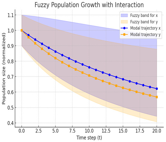
Figure 4.
Fuzzy population growth with interaction, showing modal trajectories (solid lines) and uncertainty bands (shaded areas) that illustrate positivity, boundedness, and the effect of fuzzy parameters.
Remark 6.
It is important to note that the logarithmic operation appearing in system (2) is applied only to positive arguments. More precisely, terms of the form and (or equivalently, in the application model, and ) are well-defined and positive whenever and . This assumption is natural in population and fuzzy dynamical systems, in which all state variables represent non-negative quantities such as population densities or interaction intensities. Consequently, the logarithmic terms remain positive and bounded, preserving the positivity of the fuzzy trajectories and ensuring that the scaling used in Theorem 2 remains valid under the stated conditions. Therefore, the existence of a positive fuzzy solution is guaranteed within the admissible range of the parameters.
6. Conclusions
In this paper, we conducted a comprehensive analysis of a class of two-dimensional nonlinear fuzzy difference equations characterized by logarithmic interactions. By employing the theoretical framework of fuzzy number characterization and analyzing the corresponding -cut representations, we rigorously established the existence and uniqueness of positive fuzzy solutions for arbitrary positive fuzzy initial conditions. Furthermore, we demonstrated that the positive solutions exhibit both boundedness and persistence. These theoretical findings were supported by numerical simulations that illustrated the qualitative behavior of solutions and confirmed the validity of the analytical results. The contributions of this work lie not only in extending the theoretical framework of fuzzy difference equations but also in providing insights into the dynamic behavior of such systems in the presence of fuzziness and nonlinear interactions. The analytical techniques developed in this study may serve as a foundation for studying more complex fuzzy discrete-time models with coupled dynamics, memory effects, or stochastic perturbations. Future research may build upon this work in several promising directions. One avenue is to extend the current analysis to higher-dimensional fuzzy difference systems that incorporate more general forms of nonlinear coupling between variables. Another important direction involves studying the asymptotic stability and global attractivity of positive equilibrium points under varying parameter regimes, which could offer deeper insights into the long-term behavior of such systems. Additionally, applying the theoretical findings to real-world problems, particularly in areas such as population dynamics, economics, and engineering systems subject to uncertainty and discrete-time evolution, holds significant potential for both theoretical advancement and practical impact. A population growth example confirms that the proposed fuzzy difference system produces positive, bounded, and realistic trajectories even under parameter uncertainty.
Author Contributions
Writing—original draft preparation, Y.A. and A.G. All authors have read and agreed to the published version of the manuscript.
Funding
This work was supported and funded by the Deanship of Scientific Research at Imam Mohammad Ibn Saud Islamic University (IMSIU) (grant number IMSIU-DDRSP2502).
Data Availability Statement
The original contributions presented in this study are included in the article. Further inquiries can be directed to the corresponding author.
Conflicts of Interest
The authors declare no conflicts of interest.
References
- Elaydi, S. An Introduction to Difference Equations; Springer: New York, NY, USA, 2005. [Google Scholar]
- Grove, E.A.; Ladas, G. Periodicities in Nonlinear Difference Equations; Chapman and Hall/CRC: New York, NY, USA, 2005. [Google Scholar]
- Kocic, V.L.; Ladas, G. Global Behavior of Nonlinear Difference Equations of Higher Order with Applications; Kluwer Academic Publishers: Dordrecht, The Netherlands, 1993. [Google Scholar]
- Kulenovic, M.R.S.; Ladas, G. Dynamics of Second Order Rational Difference Equations with Open Problems and Conjectures; Chapman Hall-CRC: New York, NY, USA, 2002. [Google Scholar]
- Althagafi, H.; Ghezal, A. Stability analysis of biological rhythms using three-dimensional systems of difference equations with squared terms. J. Appl. Math. Comput. 2025, 71, 3211–3232. [Google Scholar] [CrossRef]
- Alraddadi, R. The logTG-SV model: A threshold-based volatility framework with logarithmic shocks for exchange rate dynamics. AIMS Math. 2025, 10, 19495–19511. [Google Scholar] [CrossRef]
- Elsayed, E.M. Expression and behavior of the solutions of some rational recursive sequences. Math. Methods Appl. Sci. 2016, 39, 5682–5694. [Google Scholar] [CrossRef]
- Gümüş, M.; Abo-Zeid, R. Global behavior of a rational second order difference equation. J. Appl. Math. Comput. 2020, 62, 119–133. [Google Scholar] [CrossRef]
- Gümüş, M.; Abo-Zeid, R. An explicit formula and forbidden set for a higher order difference equation. J. Appl. Math. Comput. 2020, 63, 133–142. [Google Scholar] [CrossRef]
- Althagafi, H. Dynamics of difference systems: A mathematical study with applications to neural systems. AIMS Math. 2025, 10, 2869–2890. [Google Scholar] [CrossRef]
- Stefanidou, G. A fuzzy difference equation of a rational form. J. Nonlinear Math. Phys. 2005, 12, 300–315. [Google Scholar] [CrossRef]
- Wang, C.; Su, X.; Liu, P.; Hu, X.; Li, R. On the dynamics of a five-order fuzzy difference equation. J. Nonlinear Sci. Appl. 2017, 10, 3303–3319. [Google Scholar] [CrossRef]
- Yalçınkaya, I.; El-Metwally, H.; Tollu, D.T.; Ahmad, H. Behavior of solutions to the fuzzy difference equation zn+1=A+Bzn−m. Math. Notes 2023, 113, 292–302. [Google Scholar] [CrossRef]
- Atpinar, S.; Yazlik, Y. Qualitative behavior of exponential type of fuzzy difference equations system. J. Appl. Math. Comput. 2023, 69, 4135–4162. [Google Scholar] [CrossRef]
- Zhang, Q.; Ouyang, M.; Pan, B.; Lin, F. Qualitative analysis of second-order fuzzy difference equation with quadratic term. J. Appl. Math. Comput. 2023, 69, 1355–1376. [Google Scholar] [CrossRef]
- Usman, M.; Khaliq, A.; Azeem, M.; Swaray, S.; Kallel, M. The dynamics and behavior of logarithmic type fuzzy difference equation of order two. PLoS ONE 2024, 19, e0309198. [Google Scholar] [CrossRef]
- Althagafi, H.; Ghezal, A. Global stability of a system of fuzzy difference equations of higher-order. J. Appl. Math. Comput. 2025, 71, 1887–1909. [Google Scholar] [CrossRef]
- Attia, N.; Ghezal, A. Qualitative behavior of bidimensional rational fuzzy difference equations. Abstr. Appl. Anal. 2025, 2025, 7666805. [Google Scholar]
- Balegh, M.; Ghezal, A. Dynamical analysis of a system of fuzzy difference equations with power terms. Int. J. Dynam. Control 2025, 13, 364. [Google Scholar] [CrossRef]
- Ouyang, M.; Zhang, Q.; Cai, M.; Zeng, Z. Dynamic analysis of a fuzzy Bobwhite quail population model under g-division law. Sci. Rep. 2024, 14, 9682. [Google Scholar] [CrossRef]
- Zhang, Q.; Pan, B.; Ouyang, M.; Lin, F. Large time behavior of solution to second-order fractal difference equation with positive fuzzy parameters. J. Intell. Fuzzy Syst. 2023, 45, 5709–5721. [Google Scholar] [CrossRef]
- Zhang, Q.; Ouyang, M.; Zhang, Z. On second-order fuzzy discrete population model. Open Math. 2022, 20, 125–139. [Google Scholar] [CrossRef]
- Bede, B. Mathematics of Fuzzy Sets and Fuzzy Logic; Springer: London, UK, 2013. [Google Scholar]
- Diamond, P.; Kloeden, P. Metric Spaces of Fuzzy Sets; World Science: Singapore, 1994. [Google Scholar]
- Klir, G.; Yuan, B. Fuzzy Sets and Fuzzy Logic. Theory and Applications; Prentice Hall PTR: Upper Saddle River, NJ, USA, 1995. [Google Scholar]
- Negoita, C.V.; Ralescu, D. Applications of Fuzzy Sets to Systems Analysis; Birkhauser Verlag: Besel, Switzerland, 1975. [Google Scholar]
- Stefanini, L. A generalization of Hukuhara difference and division for interval and fuzzy arithmetic. Fuzzy Sets Syst. 2010, 161, 1564–1584. [Google Scholar] [CrossRef]
- Wu, C.; Zhang, B. Embedding problem of noncompact fuzzy number space E. Fuzzy Sets Syst. 1999, 105, 165–169. [Google Scholar] [CrossRef]
- Kaleva, O. Fuzzy differential equations. Fuzzy Sets Syst. 1987, 24, 301–317. [Google Scholar] [CrossRef]
- Goetschel, R.; Voxman, W. Elementary fuzzy calculus. Fuzzy Sets Syst. 1986, 18, 31–43. [Google Scholar] [CrossRef]


Disclaimer/Publisher’s Note: The statements, opinions and data contained in all publications are solely those of the individual author(s) and contributor(s) and not of MDPI and/or the editor(s). MDPI and/or the editor(s) disclaim responsibility for any injury to people or property resulting from any ideas, methods, instructions or products referred to in the content. |
© 2025 by the authors. Licensee MDPI, Basel, Switzerland. This article is an open access article distributed under the terms and conditions of the Creative Commons Attribution (CC BY) license (https://creativecommons.org/licenses/by/4.0/).