Article

Composite Test Functions for Benchmarking Nonlinear Optimization Software

by
János D. Pintér
Department of Management Science and Information Systems, Rutgers University, 100 Rockafeller Rd, Piscataway, NJ 08854, USA
Mathematics 2025, 13(21), 3524; https://doi.org/10.3390/math13213524
Submission received: 10 July 2025 / Revised: 22 October 2025 / Accepted: 29 October 2025 / Published: 3 November 2025
(This article belongs to the Special Issue Innovations in Optimization and Operations Research)

Abstract

Nonlinear optimization (NLO) is widely applicable to model and solve decision problems arising in engineering, economic, financial, and scientific studies. Due to the general scope of NLO, optimization model difficulty varies substantially, requiring the utilization of robust, efficient, and flexible solver software. In order to develop constructive guidelines regarding suitable software choices, broad, representative, and reproducible classes of test problems are needed. In this article, we propose flexible and expandable classes of composite test functions, based on earlier introduced or brand-new test problems with known solutions. In our illustrative tests, we use the high-level computing system Mathematica as a model development platform, with some of its readily available NLO solver options. The suggested general approach can be easily adapted to develop benchmarking studies using other modeling environments, test model collections, and solver options.

1. Nonlinear Optimization: A Generic Model

Quantitative decision problems (considered in a finite-dimensional real decision space) are frequently described by a corresponding optimization model. According to this paradigm, the best decision modeled by a real n-vector xRn is sought, which satisfies a given set of feasibility constraints, and minimizes (or maximizes) the value of a given objective function. For consistency, we will discuss minimization problems stated in a standardized form. A corresponding concise, symbolic optimization model statement is
(1)
Minimize f(x) subject to xD.
Here f: RnR denotes the objective function of the decision problem, and DRn is the set of feasible decisions. We will assume that D is defined by given finite variable bounds set on x, i.e., lxu, and by a set of general constraint functions g(x) = (g1(x), …, gm(x)).
(2)
D: = {lxu, g(x) ≤ 0}.
In (2), all inequality relations are interpreted component-wise; in other words, l, x, and u are n-vectors, and g is a vector-valued mapping from Rn to Rm, so that in (2), 0 ∈ Rm. For added clarity, the detailed form of the relations shown concisely by (2) is
−∞ < lixiui < ∞ for i = 1, …, n, and gj(x) ≤ 0 for j = 1, …, m.
We will also assume that all model functions f and g are continuous over the box region [l, u]⊂Rn, and that the set of feasible solutions D is non-empty. In (2), the box constraints x ∈ [l, u] are always required, but the general constraints g may be absent, thereby leading to (often much simpler) box-constrained optimization models.

2. Convex vs. Nonconvex Models

In the NLO context, we tacitly assume that at least one of the functions f, g1, …, gm is nonlinear. Further specifications of the generic NLO model (1) and (2) lead to two complementary categories: convex optimization models (in which all functions f, g1, …, gm are convex, whereby D is convex) and nonconvex optimization models (in which f is not convex and/or D is not convex).
Let us remark that, obviously, [l, u] is a convex set. If all components of g are convex functions, then each set defined by the relations gj(x) ≤ 0 is convex in Rn, for j = 1, …, m; consequently, D—as the intersection of convex sets—is convex. However, if f and/or some components of g are not convex over [l, u], then the corresponding model often becomes nonconvex. Observe that it could still happen that the resulting model is convex, although formulated with some nonconvex functions. Consider, e.g., the simple illustrative one-variable optimization problem min sin(x) s.t. 0 ≤ x ≤ 1, cos(x) ≤ 0.7. This model is convex on 0 ≤ x ≤ 1, and its unique optimum value is x* = sin(arccos(0.7)) ~ 0.714143.
Obviously, NLO encompasses both convex and nonconvex models, even if many researchers traditionally consider only convex models under the name NLO. Convex models include linear optimization models as a special case.
Without going into further details, let us also note that technically all optimization models with binary decision variables z∈{0,1} can be reformulated by introducing, for each variable z, its continuous relaxation 0 ≤ z ≤ 1, and the nonconvex inequality constraint z(1 − z) ≤ 0.
Our present study is focused on continuous NLO models. Due to the very general definition of the NLO model class, the difficulty of solving NLO models can vary to a substantial extent. As Rockafellar [1] noted, “the great watershed in optimization isn’t between linearity and nonlinearity, but convexity and nonconvexity”. The essential difference between convex and nonconvex models is due to the fact that while convex models typically have a single optimal solution (or “equivalent” solutions, in terms of having a unique optimum value), nonconvex models could have a large (frequently a priori unknown) number of local optima with different optimum values.
To illustrate the latter scenario, consider the optimization problem min x sin(x) s.t. 0 ≤ x ≤ 100. Figure 1 shows the graph of the nonconvex, multimodal objective function x sin(x). (All calculations and visual examples presented in this article have been developed by the author, using Mathematica, by Wolfram Research [2]).
For clarity, next, we recall the formal definitions of local and global optima.
A vector xl*D is a locally optimal solution of models (1) and (2), if there exists a neighborhood of xl* (such as a suitable n-dimensional sphere B centered at xl*) so that xl* is the best point in the intersection of B and the feasible set D; that is, f(xl*) ≤ f(x) holds for all xDB.
A vector xg*D is a globally optimal solution of models (1) and (2), if xg* is the best solution point in the entire feasible set D; in other words, f(xg*) ≤ f(x) holds for all points xD.
If it is clear from the context of the discussion whether we refer to a globally or locally optimal solution of an NLO model, then the corresponding solution will be simply denoted by x*. If there are multiple non-equivalent local solutions to a nonconvex NLO model (as illustrated by Figure 1), then the best of these is the global solution. Ideally, this is the solution to aim for whenever possible.
The classical Bolzano–Weierstrass theorem implies that the basic analytical assumptions postulated above regarding models (1) and (2) guarantee that their globally optimal solution set X*D is non-empty (consult, e.g., Galewski [3], or the concise MathWorld entry by Rowland and Weisstein [4]). In many well-posed NLO models, X* consists of a unique globally optimal solution x*. There are situations, however, when different globally optimal solutions exist, e.g., a system of nonlinear equations could have multiple solutions. In similar scenarios, additional considerations can be invoked if needed, to choose a preferred solution[s] among the formally equivalent global solutions in the set X*.
Let us emphasize that the existence of X* does not mean that it is necessarily straightforward to find it, or even one of its elements x*. In global (multimodal) optimization problems, analytical methods—based on derivative information—are typically not applicable to find points of X*, except in textbook examples. (Again, think of a system of nonlinear equations which could have an unknown number of solutions, as well as “pseudo-solutions” with non-zero residual error.)
Due to their structure and unique optimum value, convex NLO models of the forms (1) and (2) are “easy” to handle numerically. In principle, a suitable local scope search algorithm can be started from an arbitrary initial guess x0D of the optimal solution x*, proceeding along a sequence of descent directions and applying some line search technique. Textbooks on nonlinear local optimization discuss suitable search methods (consult, e.g., Nocedal and Wright [5].
Although many practically relevant NLO models are convex, there also exist many models that are not convex and possess a large (perhaps unknown) number of local and global optima. In contrast, solving such models is “hard”, requiring global scope search strategies. As Figure 1 illustrates, local scope optimization algorithms could miss the optimal solution; instead, a proper global search method should be used.
Within the comprehensive NLO problem category, the objective of global optimization (GO) is to find the “absolutely best” solution of provably or potentially multiextremal problems. In contrast, local optimization (LO) is aimed “only” at finding local solutions to NLO problems, noting that even this may be numerically challenging depending on the actual model structure and size.
In recent decades, NLO—specifically emphasizing here the topic of continuous GO—has become an area of intensive research. For in-depth discussions of GO model classes, solution approaches, and applications, we refer to the following works: Horst et al. [6], Horst and Pardalos [7], Pintér [8], Kearfott [9], Floudas [10], Strongin and Sergeyev [11], Pardalos and Romeijn [12], Tawarmalani and Sahinidis [13], Zabinsky [14], Neumaier [15], Liberti and Maculan [16], Zhigljavsky and Žilinskas [17], Hendrix and G.-Tóth [18], Weise [19], Schäffler [20], Locatelli and Schoen [21], Sergeyev et al. [22], Paulavičius and Žilinskas [23], Sergeyev and Kvasov [24], Stripinis and Paulavičius [25], and Stein [26]. We note that the book chapter by Neumaier [15] and the electronic book by Weise [19] are available as free downloads (to avoid an even longer list of GO references, only a selection of works published in the last three decades is listed above in chronological order; most of these works also include some discussions of software implementations, test problems, and/or real-world applications).
To motivate the forthcoming discussion, we present two further model examples. Consider, first, the following box-constrained GO problem with two variables.
(3)
min f(x1, x2), −3 ≤ x1 ≤ 3, −3 ≤ x2 ≤ 3, where the objective function f is defined by
f(x1, x2) = 0.1(x12 + x22) + cos(x12x2) + sin(x1x22)
Figure 2 displays the surface plot of this function f over the feasible box region.
Compared with Figure 1 (where you can actually inspect the optimum), one can perceive the potential difficulty of finding the global minimum of such a function, even if this example is merely a two-dimensional box-constrained instance (n = 2; m = 0) of the general problem (1) and (2). Clearly, to find the global optimum using analytical tools seems very tedious, if at all possible (f(x1, x2) has many stationary points that should be analyzed one by one). Obviously, a local scope search approach, as outlined above, could easily “get stuck” at a locally optimal solution on the hilly landscape shown in Figure 2. Therefore, some global search strategy that enables the thorough exploration of the feasible box region −3 ≤ x1 ≤ 3, −3 ≤ x2 ≤ 3 seems far more suitable to produce a credible numerical solution estimate. Higher-dimensional GO problems could become increasingly difficult to solve; this aspect will be illustrated later on.
As an example, a locally optimal solution xl* is found numerically by the Mathematica function FindMinimum:
fl* = −1.1788253348193898, x1l* = −0.005503545028937059, x2l* = 2.6575778775653895.
The Mathematica function NMinimize returns the following global solution estimate:
fg* = −1.6898522366645035, x1g* = −1.6789196896160852, x2g* = −0.17255507373427434.
The method for selecting an automatic starting point for FindMinimum is not given explicitly in the Mathematica documentation. Based on inspecting the definition of f, the modeler can select as a starting point x0l = (0,0), where the potentially dominant (coercive component) term 0.1(x12 + x22) vanishes. Then, FindMinimum returns a solution estimate that is very close to the global solution estimate found by NMinimize (Such insight should be used whenever possible; the same notion applies for finding tight variable bounds).
Observe that we have to “trust” that the numerical solution returned is close to the global optimum indeed. Evidently, −2 is a simple lower bound for f, but a tighter bound may not be easy to find. For this reason alone, the ad hoc-chosen illustrative model (3) would not be ideal on its own to verify the capabilities of some optimization engine.
If we also have to consider some general function constraints g, then the model difficulty could increase considerably. To illustrate, consider the following general circle packing (GCP) model class. Our goal is to find the minimal size circle that can contain a given collection of circles in a non-overlapping arrangement. There is a substantial body of literature devoted to this problem (consult, e.g., Castillo et al. [27] that discusses the GCP problem, and several other circle packing model classes).
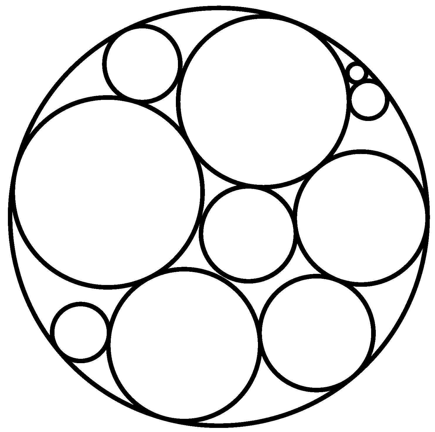
Figure 3 displays a numerically solved instance of the GCP problem with 10 packed circles.
Without going into details that are not essential for our present discussion, we remark that for a K-circle model instance, the GCP problem formulation has n = 2K + 1 decision variables, m1 = K convex constraints, and m2 = K(K − 1)/2 nonconvex constraints. In the example shown in Figure 3, K = 10; hence, n = 21 and m = m1 + m2 = 10 + 45 = 55, in addition to 2K = 20 variable bound constraints. It is easy to demonstrate that local scope solvers on their own would not be suitable to address the GCP problem class. The computational difficulty of this scalable model type rapidly increases with the model size K, leading to excessive numerical solution times even for theoretically convergent global search methods.
Except in special cases, the analytical solution of GCP instances (and similar packing problems) remains unknown, and we have to accept conjectured numerical solutions. The Packomania website maintained by Specht [28] presents a collection of challenging packing models—including instances of the GCP problem—with best-known numerical solutions. These solutions are based on the long-term computational efforts of many expert researchers, and improved optimum estimates are still being found. For these reasons—in this author’s opinion—GCP and similarly hard problems with unknown solutions should not be used as the sole criterion to assess solver quality (while they can serve as inspiring sources of modeling and solver competitions).
Let us add that some other packing models lead to even more difficult problems than GCP; again, their optimal solutions are unknown, and we have to rely on approximate numerical solutions. For recent discussions of some challenging packing problems with illustrative numerical results, consult, e.g., Kampas et al. [29], Pankratov et al. [30], Duriagina et al. [31], Castillo et al. [32], and Stoyan et al. [33]. Optimized packings have a range of important engineering and scientific applications: consult, e.g., Fasano [34], Fasano and Pintér [35].

3. Benchmarking Nonlinear Optimization Software

By definition, NLO is aimed at handling a vast range of problems, from simple to tremendously challenging. Many important NLO problems—including both combinatorial and continuous GO problems—are theoretically intractable (NP-hard). Hence, their exact solution would often require an exponentially increasing computational effort as model size increases, and in practice, one has to rely on approximate solution strategies that also include heuristics (For a simple example, think of setting up a procedure to assign random function values to each vertex of the unit cube [0,1]n in Rn. Then, in order to find the minimum of the assigned function values, one should check all 2n vertex function values). For expositions related to computational complexity, consult, e.g., Hochbaum [36], Skiena [37], Arora and Barak [38], and Heineman et al. [39]. A broad range of heuristic solution strategies is discussed, e.g., by Pardalos et al. [40] and Martí et al. [41].
For practical purposes, we need efficient algorithm implementations that work for relevant classes of NLO problems. Clearly, one cannot expect to find some software that solves “best” all imaginable NLO problems. Instead, one would prefer to obtain objective advice for selecting software options that are reliable, robust, and efficient (i.e., can produce sufficiently accurate solutions to relevant NLO problem instances in an acceptable timeframe).
Benchmarking and comparing optimization software products based on solving test problem collections has been an important topic for decades. Let us mention here, first, the Decision Tree for Optimization Software website, which includes a link to Benchmarks. This website has been maintained by Mittelmann [42] (earlier, jointly with Spellucci) for several decades. The Benchmarks webpage presents extensive software product and benchmarking information across many specific types of optimization problems, including continuous local and global NLO. For some history, related web links, and talks, cf. also the short historical note by Mittelmann [43], who contributed to many specific benchmarking studies.
The earliest GO studies—such as the books edited by Dixon and Szegö [44]—considered merely a handful of test problems that are now widely considered “too easy” for today’s hardware platforms and GO software products. A broad range of local and global NLO test models with known or conjectured numerical solutions have been made available, e.g., by Hock and Schittkowski [45], Schittkowski [46,47], Hansen et al. [48], Floudas et al. [49], Pintér [12], Casado et al. [50], Ali et al. [51], Neumaier et al. [52], Jamil and Yang [53], Rios and Sahinidis [54], Gould et al. [55], Audet and Hare [56]. While some of the test problems presented in these works are purely academic, others are motivated by practical applications in engineering and the sciences. Several further specific test model collections will be discussed later.

4. Selecting Test Problems

The overall solver quality of optimization software can be objectively and experimentally assessed by solving a set of widely acceptable, representative, and reproducible test models with known solutions. In addition to the preceding references on tests, Beiranvand et al. [57] systematically reviewed the benchmarking process and proposed best practices for comparing optimization algorithms (For clarity, these authors refer to actual software implementations of algorithms).
As noted above, some of the frequently used classical (but also some more recently introduced and often used) test problems can be considered “too easy”. On today’s powerful computers, all suitable optimization software products can solve these problems within seconds or much faster. Therefore, such tests should not be used exclusively to assess solver capabilities, while they may still be useful to verify basic software functionality.
At the other end of the spectrum, there exist very difficult problems, and nobody knows the provably optimal solution. Many of the packing problems mentioned earlier belong to this category: for even moderate-size problems (with tens or hundreds of variables and function constraints), theoretically convergent GO algorithm implementations on their own could require astronomical runtimes to find close approximations of the unknown optimal solution. Hence, again, these problems should be used only as part of a test battery to assess software capabilities and limitations. Since solver runtimes could become excessive, a practical efficiency measure can be defined by the estimated relative quality of results obtained within a preset runtime limit.
Next, it is also possible to use artificially generated test sets with known solutions. A major advantage of this approach is that one can create fully controllable test problems, which can be made easier or harder if required, by tuning some test model parameters. Model classes belonging to this category have been proposed, e.g., by Schoen [58], Mathar and Žilinskas [59], Pintér [12], Gaviano et al. [60], Addis and Locatelli [61], and Liang et al. [62].
Let us point out that Kampas et al. [29], proposed randomly generated multi-facility location problems with dispersion considerations. Randomization can effectively exclude the possibility of “calibrating” optimization software to a prefixed, limited-size test model library. In a sense, randomization mimics real-life circumstances, since—especially in the context of “black box” nonlinear optimization—problems could arise in some partially unpredictable fashion. Once the structure of a chosen model class is coded, randomized model instances can be directly generated, also supporting full model reproducibility.

5. Composite Test Functions

Following up on the argument for utilizing randomized test functions—as a model generation option—we can also combine test functions from different model libraries or even create randomized instances from the same broad library. Depending on the way such composite test functions are defined, we can gain access to new, perhaps surprising, expandable, and fully controllable collections of test models. For simplicity, we will illustrate this general concept by combinations of box-constrained NLO/GO models with known solutions. Combining general constrained optimization models would lead to further opportunities and challenges, including the creation of possibly infeasible new models.
Perhaps the easiest way to combine box-constrained test functions (on the same feasible set) is by simply adding their objective functions, using independent variable sets for each component function. For example, test functions f1(x) and f2(x) can be combined as f1(x) + f2(y) with the new set of variables (x, y). Obviously, this type of construction can be extended by adding an arbitrary (finite) number of test functions. Here, we have to assume and—for testing purposes, have to require—that the tested solver engine ignores the fact that f1(x) + f2(y) is a separable function, and treats it as a “black box”. Many GO solvers in their global scope search phase operate using only function evaluations, without using local derivatives of higher-order information. In such cases, the assumption applies that input (x, y) generates the response f1(x) + f2(y).
A great many other types of composite functions can be defined, of course. For example, one can consider products of test functions f1(x) and f2(y). As long as there is a unique global solution for the component functions, the global solution of the product function is known. The same would also apply to monotonically increasing transformations of functions (such as using exp(.), log(.), and so on, as the outer function in composite functions).
It is also possible to interchange decision variables. For example, if the combined set of variables in f1 and f2 is (x, y), then some components of x and y can be exchanged when defining f1(.)⊗f2(.), with the operator ⊗ acting on f1 and f2. Again, we can extend the construction to any finite number of component functions. Observe that in such (or more complex) constructions, the numerical solution may become unknown, even though the solution of each test function component is known. This situation can be seen as an unwanted complication or as a new numerical challenge.
For simplicity, in this article, we follow some straightforward recipes for combining test functions. Assuming that the component function solutions are decided a priori, or are known with sufficiently high precision, such combinations lead to test problems with readily available solutions.

6. Test Environment Options

There are several often-followed avenues to develop test model libraries and to solve model instances from a given library. Next, we briefly review some options. Our present discussion cannot cover “all possible” test platforms: for example, we do not discuss using Julia, Maple, MATLAB, Python, R, and others as optimization test environments, although there exist substantial developments also using these platforms. However, the proposed model generation and solution framework can be implemented across many test environments, including the ones listed above and the others briefly reviewed below.

6.1. Compiler-Based Development

Many core solver engines have been originally developed as stand-alone software executables or libraries, using programming languages such as C, C++, or Fortran. Such solver implementations can be built into various decision support systems and custom applications, benefiting from direct customizability, a small footprint, and a high execution speed. Here, we only mention the freely available GNU Compiler Collection (GCC) [63], which supports the use of multiple programming languages, including C, C++, Fortran, and others.
NLO test model libraries using compiler platforms have been developed by numerous authors (consult, e.g., the studies of Schittkowski [46,47] and Gould et al. [55]). Many of these models have also been incorporated into other modeling environments, including some that are mentioned below.

6.2. Modeling Environments for Optimization

There are distinct advantages to choosing this approach, since these platforms have been created for developing optimization models, and they typically offer direct links to various solvers. To illustrate, we mention here AMPL (Fourer et al. [64], AMPL Optimization [65]), GAMS (Brooke et al. [66], GAMS Development Corporation [67]), and LINGO (Schrage [68], LINDO Systems [69]). To illustrate the use of these systems in benchmarking studies, we mention a few examples. For the AMPL modeling environment, Vanderbei [70] has made available a substantial NLO test model collection, including benchmarking results. Floudas et al. [49] present a categorized collection of NLO test problems: these models have been implemented by the authors using the GAMS modeling language. LINDO Systems [69] also offers an extensive LINGO model library, including models discussed in several prominent textbooks. The AMPL and GAMS websites also offer a rich collection of coded model examples.

6.3. Excel

Spreadsheets are extensively used by business organizations as the primary modeling platform. Among many other features, Excel also has optimization capabilities. Frontline Systems [71], the developers of the core Excel solver engine, also offer the Premium Solver Platform (a collection of more advanced solver options), and other tools related to decision support. Excel model examples are made available by numerous textbook authors, and also by Frontline Systems.

6.4. Integrated Computing Environments

Integrated scientific–technical computing systems such as Maple, Mathematica, and MATLAB—in addition to an impressive range of other features—can also perform optimization, either using built-in functionality or by invoking add-on products. Textbook authors discussing optimization using these systems present many examples; further examples are documented on the respective product websites. In this article, we use Mathematica to develop and solve illustrative sets of composite test functions.

7. Illustrative Models and Results

7.1. A Composite Model Function Class

Next, we introduce a class of relatively simple (though viewed as “black box” functions, not trivial) composite test functions based on combining test problems with known solutions. Specifically, following up on our earlier numerical experiments described in [12], we propose the following class of n-dimensional parameterized objective functions for NLO tests over some feasible box region lxu:
(4)
f(x) = si=1,n (xixi*)2 + ∑k=1,kmax ak sin2[bk Pk(x − x*)].
In (4), s > 0, ak > 0, and bk > 0 for k = 1 and kmax (with a chosen kmax > 0 integer) are scalar parameters chosen to make a test problem more or less difficult by adjusting their values. Specifically, increasing the value of the scale parameter s makes the function more similar to an “easy” separable convex quadratic function. Increasing the amplitude multiplier ak for any k = 1, …, kmax results in a higher effect of the added oscillating terms, while increasing bk for any k = 1, …, kmax leads to higher oscillations of the arguments in the squared trigonometric terms. Finally, Pk(.) denotes an in-principle arbitrary function that attains its unique minimum with value 0 at x = x*, for k = 1, …, kmax.
The outlined “recipe” offers substantial flexibility in defining test functions. We will present illustrative examples below. Some of these examples are directly based on [4], while others extend this model toward more complicated functions.
Observe that all objective functions following the general structure described above have a unique global minimum at x = x*, with an optimum value of 0. Furthermore, a number of local optima can be created depending on the parameterization (s, ak, and bk) and the embedded functions Pk(.) chosen. The global solution x* can either be fixed or generated randomly. In our numerical experiments, we follow the randomization option.
Instead of s, a set of values si > 0 i = 1,n could also be introduced, to obtain somewhat more general (although still separable) quadratic functions. More generally, instead of the first separable summation term in (4), a positive definite coercive function could be used that attains its unique minimum value 0 at x*, while f(x)→∞ as ║x − x*║→∞. Such a coercive objective function structure is common in numerous practical applications of global optimization (e.g., in model calibration problems).
To simply illustrate the generation of composite test functions, first, we add two univariate test functions, each with separate arguments, as defined by (4). Each of the univariate component functions follows the simple formula.
(5)
f = s(xxopt)2 + a(sin(b(xxopt)2))2.
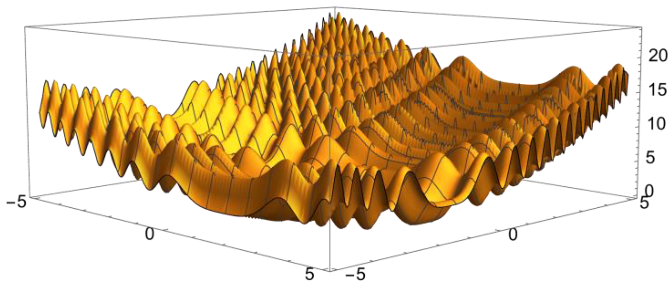
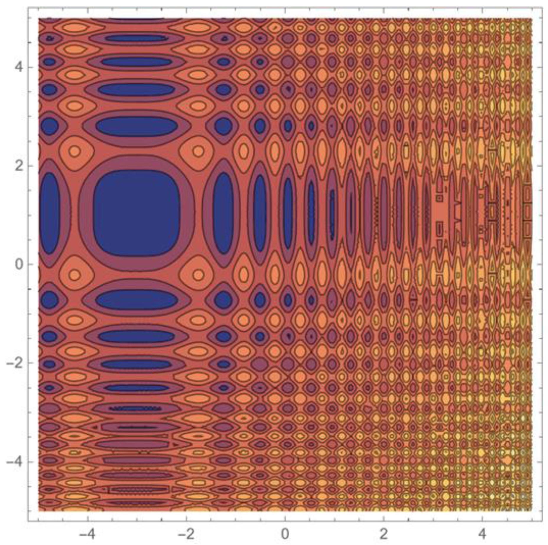
The parameterization of both functions is defined by xopt = l + RandomReal[](u-l), noting that the Mathematica function RandomReal [] returns an algorithmically generated pseudorandom real number between 0 and 1. Figure 4 displays a one-dimensional test function instance; Figure 5 and Figure 6 show, respectively, the surface plot and contour plot of a composite test function based on two of the one-dimensional test functions, with a component-wise randomly generated solution point x*.
The proposed class of test functions can be made “easy” or “challenging” by selecting their parameters. Given that, by assumption, we consider the generated functions as black boxes, higher-dimensional composite functions—especially with argument exchanges—definitely could become even more challenging for NLO software. This point will also be illustrated later.
We implemented the outlined test model construction in Mathematica, creating two-variable composite functions by simply adding two univariate test functions, i.e., f12(x,y) = f1(x) + f2(y). In our numerical tests presented here, we used Mathematica’s local scope solver FindMinimum and the global solver NMinimize. Below, we summarize the test environment information, test setup parameters, and the illustrative results obtained based on sequences of test problem runs. Further details will be made available upon request.

7.2. Test Environment

Computer hardware: Dell Precision 3560, 11th Gen Intel(R) Core(TM) i7-1185G7 @ 3.00 GHz, 1.80 GHz processor, 32 GB RAM. (Manufacturer: Dell Technologies, global headquarters: 1 Dell Way, Round Rock, TX, USA).
Operating System: Microsoft Windows 11 Enterprise (64-bit OS, x64-based processor) (Version: 24H2, Installed on: 22 January 2025, OS build: 26100.6899).
Mathematica Version: 14.2.0 for Microsoft Windows (64-bit) (26 December 2024).

7.3. Two-Variable Model Examples

The core Mathematica code is included below, with added comments. We note that in Mathematica code, the semicolon symbol (;) suppresses the resulting output of an input code line[s] when this is preferred.
The maximum number of iterations is set to the value maxit: each iteration includes a test problem generation step, followed by its solution.
maxit = 1000;
The objective function value numerical error tolerance is here set to 10−8:
Erroreps = N[(10)^−8];
The test function component 1 parameters are
lb1 = −5; ub1 = 5; s1 = 0.15; a1 = 3; b1 = 0.5;
Bounds lb1 and ub1 are used in a random solution generator:
x o p t = l b 1 + R a n d o m R e a l [ ] ( u b 1 l b 1 ) ; x o p t r = x o p t
Test function component 1 is
t e s t f c t 1 = s 1 x x o p t r 2 + a 1 S i n b 1 x x o p t r 2 2
The test function component 2 parameters are
lb2 = −5; ub2 = 5; s2 = 0.25; a2 = 5; b2 = 1;
Bounds lb2 and ub2 are used in a random solution generator:
y o p t = l b 1 + R a n d o m R e a l [ ] ( u b 1 l b 1 ) ; y o p t r = y o p t
Test function component 2 is
t e s t f c t 2 = s 2 y y o p t r 2 + a 2 S i n b 2 y y o p t r 2 2

Illustrative Test Results

Number of test problems: 1000, in each test run sequence.
Test run Local solver success rate *Global solver success rate *
10.180 (i.e., 180 out of 1000)0.512 (i.e., 512 out of 1000)
20.1580.558
30.1750.534
40.1600.515
50.1780.562
* Successful solution is reported if the numerical optimum value returned is less than eps = 10−8.
Our numerical experiments show that, for the given class of (rather simple) test problems, the local solver FindMinimum understandably more often misses the global solution, while the global solver NMinimize finds it to the preset 10−8 precision in about half of the test run instances. The runtimes for each sequence of 1000 test problems are between 35 and 45 s on the hardware and software platform reported above (runtimes also depend on running simultaneously other applications).
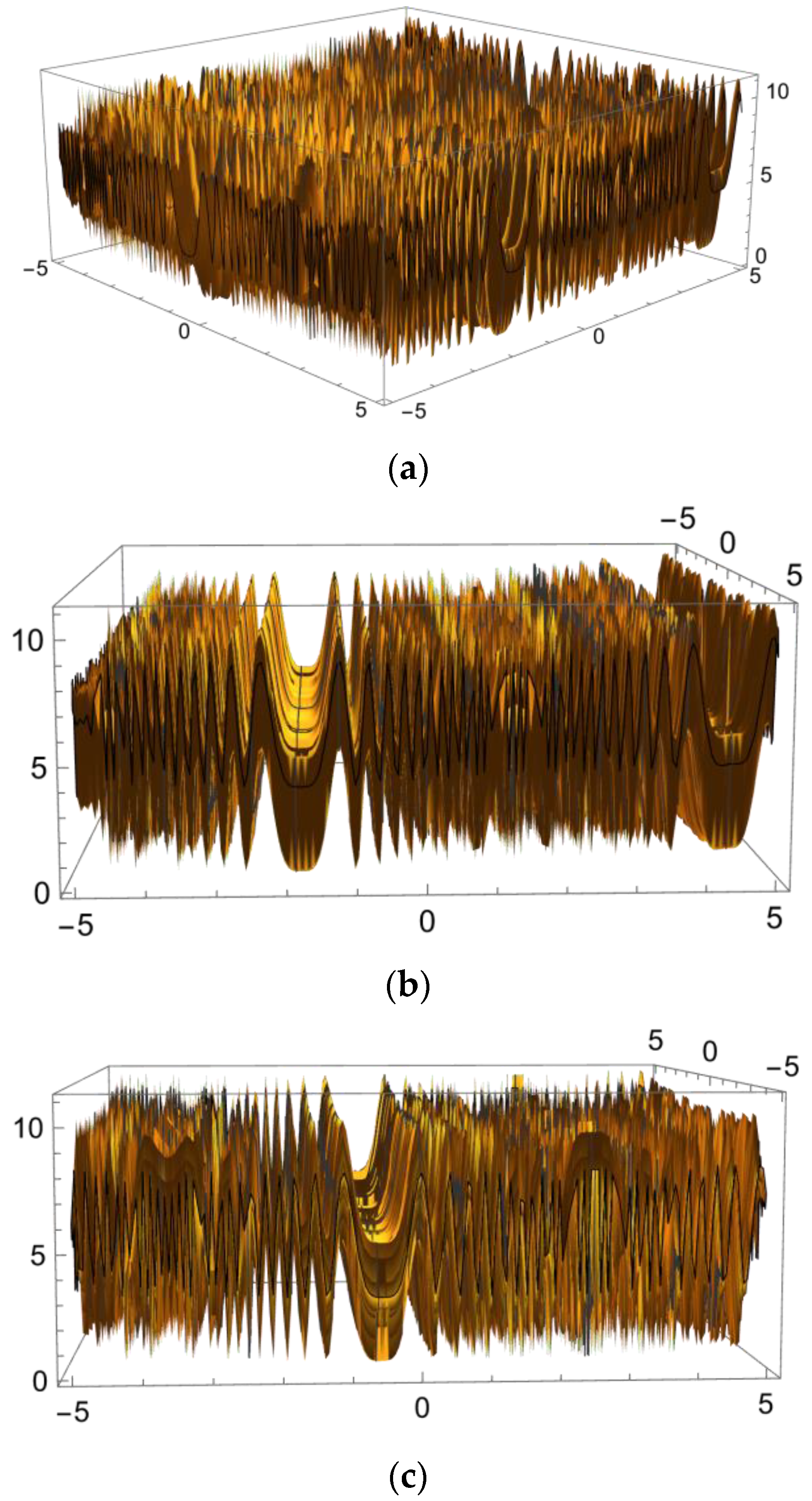
Mathematica’s numerical optimization functions are designed to handle—and, whenever possible, exploit—the separability properties of objective functions (This fact, to my knowledge, is not directly reported in the standard built-in Mathematica documentation; however, it is mentioned on several Internet sites). To illustrate, Figure 7a shows a seemingly hard instance of a randomly generated test function built as described above, but with a different parameterization. However, checking coordinate-wise cross-sections (Figure 7b,c), a well-defined region of attraction of the global optima for each univariate component functions could be identified by inspection.

7.4. Three-Variable Model Examples

Figure 7 illustrates an important point mentioned earlier: to test solvers that are able to exploit separable model structure, one has to use (also) non-separable test functions.
For this reason, next we consider randomly generated three-variable models, which extend the model form (4). This, of course, can be achieved in a great many ways. Here, we use the illustrative component functions defined below:
testfct1 = s1*((x − xoptr) + 7*(y − yoptr) − 4*(z − zoptr))^2
+ a1*(Sin[b1*(x^2*(x − yoptr)*z^3 − xoptr^2*(xoptr − y)*zoptr^3)])^2;
testfct2 = s2*(x − xoptr + 3*(yoptr − y) − 5*(z − zoptr))^2
+ a2*(Sin[b2*(x*(xoptr − y)^2*z − xoptr*(x − yoptr)^2*zoptr)])^2;
testfct3 = s3*((x − xoptr) − (y − yoptr) + 5*(z − zoptr))^2
+ a3*(Sin[b3*(x*(xoptr − y + zoptr)*z^2 − xoptr*(x − yoptr + z)*zoptr^2)])^2;
testfct = testfct1 + testfct2 + testfct3;
The initialization code is analogous to the code shown previously and is, hence, omitted. The reader will notice that we use different linear combinations of the variables in the first term of each component function, while in the trigonometric terms, we use nonlinear combinations of the variables. The eventual composite test function is simply the sum of the components.
These non-separable test functions can be expected to become harder to handle than the separable functions discussed above, as our test results show.

Illustrative Test Results

Number of test problems: 100.
Test runLocal solver success rate *Global solver success rate *
10.00 (i.e., 0 out of 100)0.28 (i.e., 28 out of 100)
20.000.33
30.000.32
40.000.37
50.000.35
* Successful solution is reported if the numerical optimum value returned is less than eps = 10−8.
Observe that now the local solver is unable to find the global solution, while—for this particular type of test problem—the global solver also fails more often. This fact is not meant to “criticize” Mathematica’s strong numerical optimization capabilities. It is easy to “fabricate” hard global optimization test models with complicated interactions among the variables that no solver can solve reliably, within a realistic time frame (We use the optimization functions FindMinimum and NMinimize with their default settings).
The solution times have become longer; the runtimes for each sequence of 100 test problems now vary between 50 and 70 s on the hardware and software platform reported above, also depending on the tasks performed simultaneously. This is the reason for choosing shorter (100 vs. 1000) test run cycles, which clearly demonstrate the point.

7.5. Five-Variable Model Examples

To further illustrate the effect of increasing the model dimension and the difficulties implied, we also present a set of test problems with n = 5 variables. Here, we use the following extended instance of model (4).
testfct1 = s1*((x − xoptr) − 3*(z − zoptr) + 5*(u − uoptr) − 7*(y − yoptr) +
9*(y − yoptr))^2 +
a1*(Sin[b1*(x^2*y^2*v*u*z − xoptr^2*yoptr^2*voptr*uoptr*zoptr)])^2;
testfct2 = s2*(x − yoptr − xoptr + y)^2 +
a2*(Sin[b2*(x*y*u + v*z − xoptr*yoptr*uoptr − voptr*zoptr)])^2;
testfct3 = s3*(x − xoptr + 2*(yoptr − y) + 3*(z − zoptr) + (u − uoptr) +
5*(voptr − v))^2 +
a3*(Sin[b3*(x*(yoptr − y + uoptr − u)*z − (x − xoptr + z − zoptr)*
u*v)])^2;
testfct4 = s4*((v − voptr) + (z − zoptr) + 6*(x + y − xoptr − yoptr))^2 +
a4*(Sin[b1*(x^2*u^2*y − xoptr^2*uoptr^2*yoptr)])^2;
testfct5 = s5*((voptr − v) + 5*(xoptr − x) − 11*(z − zoptr))^2 +
a5*(Sin[b2*(x*u*v*y*z^2 − xoptr*uoptr*voptr*yoptr*zoptr^2)])^2;
testfct = testfct1 + testfct2 + testfct3 + testfct4 + testfct5;
These composite test functions can be expected to become even harder than the three-variable models discussed above. Obviously, numerical difficulty is influenced by both the chosen model form and its parameters.

Illustrative Test Results

Number of test problems: 100.
Test runLocal solver success rate *Global solver success rate *
10.00 (i.e., 0 out of 100)0.06 (i.e., 6 out of 100)
20.000.06
30.000.07
40.000.05
50.000.02
* Successful solution is reported if the numerical optimum value returned is less than eps = 10−8.
Not surprisingly, the local solver is unable to find the global solution with the required precision, while—for this particular type of test problem—the global solver also fails even more often.
The solution times have become longer; the runtimes for each sequence of 100 test problems vary between ca. 300 and 450 s (again, depending on the actual usage of the computer).
Clearly, instances from the chosen model class would be very difficult to solve in increasingly higher dimensions–arguably, for any global solver software. This is true, in spite of the fact that we discussed “only” box-constrained test models. Substantial added complexity could arise in the presence of difficult nonlinear constraints, as the circle packing example presented in Section 2 illustrates.

8. Conclusions

The practice of nonlinear optimization—specifically including global optimization—frequently leads to very hard numerical challenges. To further illustrate this point, note that there exist much harder packing problems than the GCP model class highlighted in Section 2. In such cases, no algorithm can be expected on its own to find the theoretical best solution within a reasonable time frame. Instead, high-quality optimization software—often complemented by insightful heuristics—only enables the finding of credible solution estimates. Under real-life circumstances, this is often the best outcome that can be expected. As John von Neumann [72] famously stated, “Truth… is much too complicated to allow anything but approximations…”. When facing hard optimization problems, practical solver comparisons can be based on the relative quality of the numerical solutions found within time-normalized tests. An alternative, more “idealistic” route is often followed by problem-solving competitions when the best solution found is reported, but often without reporting the (possibly very substantial) computational effort required.
Comprehensive software tests on a range of representative problems are important to support the development of objective software selection guidelines. In this study, we propose the introduction of composite test function classes based on existing or new test problems with known solutions. This general concept can be flexibly applied to create literally infinite collections of new test problems.
In our illustrative tests presented here, we use Mathematica as the model development and solver platform. A distinct advantage of using a high-level modeling system and parameterized collections of test functions is that once the testing framework is developed (coded), it can be readily modified by changing some model components and parameters, thereby making the resulting model collections more or less challenging. Model randomization is another useful feature, when applicable. Model visualization, when supported by the modeling platform, can help to gain additional insight about the proposed models.
The approach presented here can be adopted to develop test model collections and benchmarking studies, also using other modeling environments and their solver options. Most model development environments also support randomized tests by using (built-in or coded) reproducible pseudo-random number sequences. The highlighted and illustrated model development features support the efficient generation of test model sequences, thereby assisting the exploration of an ever-increasing range of optimization challenges.

Funding

This research received no external funding.

Data Availability Statement

The original contributions presented in this study are included in this article. Further inquiries can be directed to the corresponding author.

Acknowledgments

I have been planning to work on a topical article for quite some time. Alas, substantial (mostly positive) life twists and turns interfered. I wish to acknowledge Victor Zverovich for the topical discussions and tests conducted years ago in the AMPL modeling environment. Our paths diverged, but I would be glad to revisit and to complete those AMPL tests if/when opportune. Victor’s LinkedIn page, (https://www.linkedin.com/in/zverovich/, accessed on 1 July 2025) says “Victor (doesn’t read messages) Zverovich”, but perhaps some readers of this opus know how to contact him, or he just happens to read it himself. (For clarity, let me add that the idea of composite test functions—as presented and implemented here—was proposed by me, and that in the present study, I introduced entirely different test models coded in Mathematica, from the ones discussed with and tested by Victor using AMPL). I also wish to acknowledge Ignacio Castillo, Giorgio Fasano, and Frank Kampas for research cooperation and stimulating discussions. Some of our joint research work on optimized packings is cited in this article. Frank Kampas and I also co-authored several articles using Mathematica as a model development and solver benchmarking platform (using different models and different solvers from the ones discussed here). Wolfram Research, the developers of Mathematica, has been supporting my research over several decades. Mathematica has been used to create and solve all illustrative test problems and to generate all figures presented in this article. I wish to thank the Igor Litvinchev and the other SI Editors for their kind invitation and attention to my work. Finally, I also wish to thank the reviewers of this article for all constructive comments.

Conflicts of Interest

The author declares no conflict of interest.

References

  1. Rockafellar, R.T. Lagrange multipliers and optimality. SIAM Rev. 1993, 35, 183–238. [Google Scholar] [CrossRef]
  2. Wolfram Research. Mathematica (Release 14.2); Wolfram Research: Champaign, IL, USA, 2025; Available online: https://www.wolfram.com/mathematica/ (accessed on 28 October 2025).
  3. Galewski, M. Basics of Nonlinear Optimization—Around the Weierstrass Theorem; Birkhäuser, Springer Nature: Cham, Switzerland, 2024. [Google Scholar]
  4. Rowland, T.; Weisstein, E.W. Bolzano-Weierstrass Theorem. From MathWorld—A Wolfram Web Resource. 2025. Available online: https://mathworld.wolfram.com/Bolzano-WeierstrassTheorem.html (accessed on 5 June 2025).
  5. Nocedal, J.; Wright, S.J. Numerical Optimization, 2nd ed.; Springer Science + Business Media: New York, NY, USA, 2006. [Google Scholar]
  6. Horst, R.; Pardalos, P.M.; Thoai, N.V. Introduction to Global Optimization; Kluwer Academic Publishers: Dordrecht, The Netherlands, 1995. [Google Scholar]
  7. Horst, R.; Pardalos, P.M. (Eds.) Handbook of Global Optimization; Kluwer Academic Publishers: Dordrecht, The Netherlands, 1995; Volume 1. [Google Scholar]
  8. Pintér, J.D. Global Optimization in Action; Kluwer Academic Publishers: Dordrecht, The Netherlands, 1996. [Google Scholar]
  9. Kearfott, R.B. Rigorous Global Search: Continuous Problems; Kluwer Academic Publishers: Dordrecht, The Netherlands, 1996. [Google Scholar]
  10. Floudas, C.A. Deterministic Global Optimization; Kluwer: Dordrecht, The Netherlands, 2000. [Google Scholar]
  11. Strongin, R.G.; Sergeyev, Y.D. Global Optimization with Non-Convex Constraints: Sequential and Parallel Algorithms; Kluwer Academic Publishers: Dordrecht, The Netherlands, 2000. [Google Scholar]
  12. Pintér, J.D. Global optimization: Software, test problems, and applications. In Handbook of Global Optimization, Volume 2; Pardalos, P.M., Romeijn, H.E., Eds.; Kluwer Academic Publishers: Dordrecht, The Netherlands, 2002; pp. 515–569. [Google Scholar]
  13. Tawarmalani, M.; Sahinidis, N. Convexification and Global Optimization in Continuous and Mixed-Integer Nonlinear Programming; Kluwer Academic Publishers: Dordrecht, The Netherlands, 2002. [Google Scholar]
  14. Zabinsky, Z.B. Stochastic Adaptive Search for Global Optimization; Kluwer Academic Publishers: Dordrecht, The Netherlands, 2003. [Google Scholar]
  15. Neumaier, A. Complete search in continuous global optimization and constraint satisfaction. In Acta Numerica 2004; Iserles, A., Ed.; Cambridge University Press: Cambridge, UK, 2004; pp. 271–369, preprint; Available online: https://arnold-neumaier.at/papers.html#glopt03 (accessed on 26 June 2025).
  16. Liberti, L.; Maculan, N. (Eds.) Global Optimization—From Theory to Implementation; Springer Science + Business Media: New York, NY, USA, 2006. [Google Scholar]
  17. Zhigljavsky, A.; Žilinskas, A. Stochastic Global Optimization; Springer Science + Business Media: New York, NY, USA, 2008. [Google Scholar]
  18. Hendrix, E.M.T.; G-Tóth, B. Introduction to Nonlinear and Global Optimization; Springer: Berlin/Heidelberg, Germany, 2010. [Google Scholar]
  19. Weise, T. Global Optimization Algorithms—Theory and Application. Published by the Author. Available online: https://www.researchgate.net/publication/200622167_Global_Optimization_Algorithm_Theory_and_Application (accessed on 26 June 2025).
  20. Schäffler, S. Global Optimization—A Stochastic Approach; Springer Science + Business Media: New York, NY, USA, 2012. [Google Scholar]
  21. Locatelli, M.; Schoen, F. Global Optimization: Theory, Algorithms, and Applications; Society for Industrial and Applied Mathematics: Philadelphia, PA, USA, 2013. [Google Scholar]
  22. Sergeyev, Y.D.; Strongin, R.G.; Lera, D. Introduction to Global Optimization Exploiting Space-Filling Curves; Springer Science + Business Media: New York, NY, USA, 2013. [Google Scholar]
  23. Paulavičius, R.; Žilinskas, J. Simplicial Global Optimization; Springer Science + Business Media: New York, NY, USA, 2014. [Google Scholar]
  24. Sergeyev, Y.D.; Kvasov, D.E. Deterministic Global Optimization—An Introduction to the Diagonal Approach; Springer Science + Business Media: New York, NY, USA, 2017. [Google Scholar]
  25. Stripinis, L.; Paulavičius, R. Derivative-Free DIRECT-Type Global Optimization—Applications and Software; Springer Nature: Cham, Switzerland, 2023. [Google Scholar]
  26. Stein, O. Basic Concepts of Global Optimization; Springer: Berlin/Heidelberg, Germany, 2024. [Google Scholar]
  27. Castillo, I.; Kampas, F.J.; Pintér, J.D. Solving circle packing problems by global optimization: Numerical results and industrial applications. Eur. J. Oper. Res. 2008, 191, 786–802. [Google Scholar] [CrossRef]
  28. Specht, E. Packomania. 2025. Available online: http://www.packomania.com/ (accessed on 5 June 2025).
  29. Kampas, F.J.; Pintér, J.D.; Castillo, I. Model development and solver demonstrations in class using randomized test problems. Oper. Res. Forum 2023, 4, 13. [Google Scholar] [CrossRef]
  30. Pankratov, A.; Romanova, T.; Litvinchev, I. Packing oblique 3D objects. Mathematics 2020, 8, 1130. [Google Scholar] [CrossRef]
  31. Duriagina, Z.; Pankratov, A.; Romanova, T.; Litvinchev, I.; Bennell, J.; Lemishka, I.; Maximov, S. Optimized packing titanium alloy powder particles. Computation 2023, 11, 22. [Google Scholar] [CrossRef]
  32. Castillo, I.; Pintér, J.D.; Kampas, F.J. The boundary-to-boundary p-dispersion configuration problem with oval objects. J. Oper. Res. Soc. 2024, 75, 2327–2337. [Google Scholar] [CrossRef]
  33. Stoyan, Y.; Yaskov, G.; Romanova, T.; Litvinchev, I.; Velarde Cantú, J.M.; Acosta, M.L. Packing spheres into a minimum-height parabolic container. Axioms 2024, 13, 396. [Google Scholar] [CrossRef]
  34. Fasano, G. Solving Non-Standard Packing Problems by Global Optimization and Heuristics; Springer Briefs in Optimization; Springer Science + Business Media: New York, NY, USA, 2014. [Google Scholar]
  35. Fasano, G.; Pintér, J.D. (Eds.) Optimized Packings with Applications; Springer Science + Business Media: New York, NY, USA, 2015. [Google Scholar]
  36. Hochbaum, D. Complexity and algorithms for nonlinear optimization problems. Ann. Oper. Res. 2007, 153, 257–296. [Google Scholar] [CrossRef]
  37. Skiena, S.S. The Algorithm Design Manual, 2nd ed.; Springer Science + Business Media: New York, NY, USA, 2008. [Google Scholar]
  38. Arora, S.; Barak, B. Computational Complexity: A Modern Approach; Cambridge University Press: New York, NY, USA, 2009. [Google Scholar]
  39. Heineman, G.T.; Pollice, G.; Selkow, S. Algorithms in a Nutshell, 2nd ed.; O’Reilly Media: Sebastopol, CA, USA, 2016. [Google Scholar]
  40. Pardalos, P.M.; Du, D.-Z.; Graham, R.L. (Eds.) Handbook of Combinatorial Optimization, 2nd ed.; Springer Science + Business Media: New York, NY, USA, 2013. [Google Scholar]
  41. Martí, R.; Pardalos, P.M.; Resende, M.G.C. (Eds.) Handbook of Heuristics; Springer Nature: Cham, Switzerland, 2018. [Google Scholar]
  42. Mittelmann, H.D. Decision Tree for Optimization Software. 2025. Available online: https://plato.asu.edu/guide.html (accessed on 3 July 2025).
  43. Mittelmann, H.D. Benchmarking optimization software—A (hi)story. Oper. Res. Forum 2020, 1, 2. [Google Scholar] [CrossRef]
  44. Dixon, L.C.W.; Szegö, G.P. (Eds.) Towards Global Optimisation; Elsevier North-Holland: Amsterdam, The Netherlands, 1975; Volumes 1–2. [Google Scholar]
  45. Hock, W.; Schittkowski, K. Test Examples for Nonlinear Programming Codes; Lecture Notes in Economics and Mathematical Systems; Springer: Berlin/Heidelberg, Germany, 1981; Volume 187. [Google Scholar]
  46. Schittkowski, K. More Test Examples for Nonlinear Programming; Lecture Notes in Economics and Mathematical Systems; Springer: Berlin/Heidelberg, Germany, 1987; Volume 182. [Google Scholar]
  47. Schittkowski, K. An Updated Set of 306 Test Problems for Nonlinear Programming with Validated Optimal Solutions—User’s Guide; Research Report; Department of Computer Science, University of Bayreuth: Bayreuth, Germany, 2008. [Google Scholar]
  48. Hansen, P.; Jaumard, B.; Lu, S.-H. Global optimization of univariate Lipschitz functions: II. New algorithms and computational comparison. Math. Program. 1992, 55, 273–292. [Google Scholar] [CrossRef]
  49. Floudas, C.A.; Pardalos, P.M.; Adjiman, C.S.; Esposito, W.R.; Gümüş, Z.H.; Harding, S.T.; Klepeis, J.L.; Meyer, C.A.; Schweiger, C.A. Handbook of Test Problems in Local and Global Optimization; Kluwer Academic Publishers: Dordrecht, The Netherlands, 1999. [Google Scholar]
  50. Casado, L.G.; Martínez, J.A.; García, I.; Sergeyev, Y.D. New interval analysis support functions using gradient information in a global minimization algorithm. J. Glob. Optim. 2003, 25, 345–362. [Google Scholar] [CrossRef]
  51. Ali, M.M.; Khompatraporn, C.; Zabinsky, Z.B. A numerical evaluation of several stochastic algorithms on selected continuous global optimization test problems. J. Glob. Optim. 2005, 31, 635–672. [Google Scholar] [CrossRef]
  52. Neumaier, A.; Shcherbina, O.; Huyer, W.; Vinkó, T. A comparison of complete global optimization solvers. Math. Program. Ser. B 2005, 103, 335–356. [Google Scholar] [CrossRef]
  53. Jamil, M.; Yang, X.S. A literature survey of benchmark functions for global optimisation problems. Int. J. Math. Model. Numer. Optim. 2013, 4, 150–194. [Google Scholar] [CrossRef]
  54. Rios, L.M.; Sahinidis, N.V. Derivative-free optimization: A review of algorithms and comparison of software implementations. J. Glob. Optim. 2013, 56, 1247–1293. [Google Scholar] [CrossRef]
  55. Gould, N.I.M.; Orban, D.; Toint, P.L. CUTEst: A constrained and unconstrained testing environment with safe threads for mathematical optimization. Comput. Optim. Appl. 2015, 60, 545–557. [Google Scholar] [CrossRef]
  56. Audet, C.; Hare, W. Derivative-Free and Blackbox Optimization; Springer International Publishing AG: Cham, Switzerland, 2017. [Google Scholar]
  57. Beiranvand, V.; Hare, W.; Lucet, Y. Best practices for comparing optimization algorithms. Optim. Eng. 2017, 18, 815–848. [Google Scholar] [CrossRef]
  58. Schoen, F. A wide class of test functions for global optimization. J. Glob. Optim. 1993, 3, 133–137. [Google Scholar] [CrossRef]
  59. Mathar, R.; Žilinskas, A. A class of test functions for global optimization. J. Glob. Optim. 1994, 5, 195–199. [Google Scholar] [CrossRef]
  60. Gaviano, M.; Kvasov, D.E.; Lera, D.; Sergeyev, Y.D. Software for generation of classes of test functions with known local and global minima for global optimization. ACM Trans. Math. Softw. 2003, 29, 469–480. [Google Scholar] [CrossRef]
  61. Addis, B.; Locatelli, M. A new class of test functions for global optimization. J. Glob. Optim. 2007, 38, 479–501. [Google Scholar] [CrossRef]
  62. Liang, J.J.; Qu, B.Y.; Suganthan, P.N.; Hernández-Díaz, A.G. Problem Definitions and Evaluation Criteria for the CEC 2013 Special Session on Real-Parameter Optimization; Technical Report 201212.34; Computational Intelligence Laboratory, Zhengzhou University: Zhengzhou, China; Nanyang Technological University: Singapore, 2013. [Google Scholar]
  63. Free Software Foundation (1988–2025). GCC, the GNU Compiler Collection. © Free Software Foundation, Inc. Available online: https://gcc.gnu.org/ (accessed on 28 October 2025).
  64. Fourer, R.; Gay, D.M.; Kernighan, B.W. AMPL—A Modeling Language for Mathematical Programming, 2nd ed.; Duxbury-Thomson: Pacific Grove, CA, USA, 2003; Available online: https://ampl.com/resources/books/ampl-book/ (accessed on 25 June 2025).
  65. AMPL Optimization AMPL. 2025. Available online: https://ampl.com (accessed on 5 June 2025).
  66. Brooke, A.; Kendrick, D.; Meeraus, A. GAMS: A User’s Guide; The Scientific Press: Redwood City, CA, USA, 1988; Available online: www.gams.com (accessed on 28 October 2025).
  67. GAMS Development Corporation. GAMS (The General Algebraic Modeling Language). 2025. Available online: https://www.gams.com/products/gams/gams-language/ (accessed on 25 June 2025).
  68. Schrage, L. Optimization Modeling with LINGO. 2002. Available online: https://www.lindo.com/downloads/Lingo_Textbook_5thEdition.pdf (accessed on 25 June 2025).
  69. LINDO Systems. LINGO—Optimization Modeling Software for Linear, Nonlinear, and Integer Programming. 2025. Available online: https://www.lindo.com/index.php/products/lingo-and-optimization-modeling (accessed on 25 June 2025).
  70. Vanderbei, R.J. Benchmarks for Nonlinear Optimization. 2025. Available online: https://vanderbei.princeton.edu/bench.html (accessed on 1 July 2025).
  71. Frontline Systems. Premium Solver Platform. 2025. Available online: https://www.solver.com/premium-solver-platform (accessed on 25 June 2025).
  72. Neumann, J. The mathematician. In Works of the Mind; Heywood, R.B., Ed.; University of Chicago Press: Chicago, IL, USA, 1947; pp. 180–196. [Google Scholar]
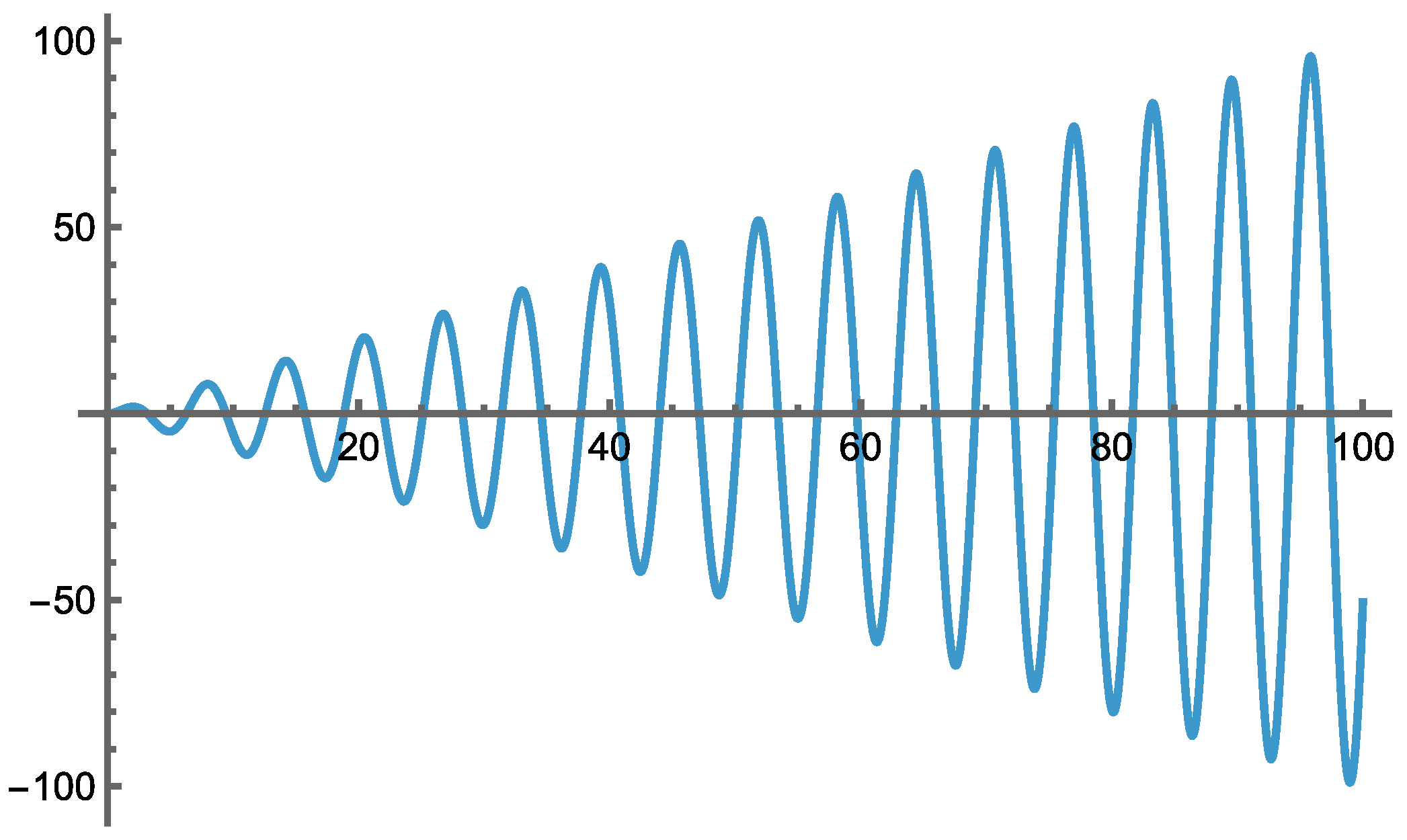
Figure 1. Graph of the nonconvex function x sin(x), 0 ≤ x ≤ 100.
Mathematics 13 03524 g001
Figure 2. An illustrative two-variable box-constrained GO problem.
Mathematics 13 03524 g002
Figure 3. A numerically solved GCP model instance.
Mathematics 13 03524 g003
Figure 4. Graph of a randomly generated one-dimensional test function, see Formula (5).
Mathematics 13 03524 g004
Figure 5. Surface plot of a randomly generated two-dimensional test function, based on adding two one-dimensional test functions, each of these being defined applying Formula (5).
Mathematics 13 03524 g005
Figure 6. Contour plot of a randomly generated two-dimensional test function, based on adding two one-dimensional test functions, each of these being defined applying Formula (5).
Mathematics 13 03524 g006
Figure 7. An instance of a randomly generated test function. (a) A general surface plot view of a randomly generated test function. (b,c) Cross-sections of the rotated surface plot indicate separability.
Mathematics 13 03524 g007
Disclaimer/Publisher’s Note: The statements, opinions and data contained in all publications are solely those of the individual author(s) and contributor(s) and not of MDPI and/or the editor(s). MDPI and/or the editor(s) disclaim responsibility for any injury to people or property resulting from any ideas, methods, instructions or products referred to in the content.