Refined One Relaxation Time-Fractional Theory for the Thermoelastic Response of Circular Cylinders with Variable Thermal Conductivity

Abstract

The fractional thermoelasticity theory is presented for the thermal response of a circular cylinder. The basic equations of the cylinder are derived from a fractional theory in the context of the generalized Lord and Shulman theory. It is taken into consideration the variable thermal conductivity of the circular cylinder. A temperature-mapping function is used for this purpose. The cylinder is subjected to an exponential decay of temperature mapping over time at its outer surface. The governing equations are solved by using the Laplace transform technique, and its inversion is carried out numerically. Numerical outcomes are computed and represented graphically for the field variables along the radial direction of the cylinder. The effects of many parameters on all thermoelastic fields are investigated. The analysis highlights the relationship between the field quantities and the radial direction of the circular cylinder, the impact of the exponential decay time, the impact of the thermal conductivity parameter, the inclusion of the fractional parameter, and the difference between the refined thermoelasticity theories.

1. Introduction

In generalized thermoelasticity, allowing thermal conductivity to vary with temperature adds complexity but makes models more realistic, especially in extreme heat conditions. When temperature gradients are large, thermal conductivity is no longer constant, making the governing equations nonlinear. Solving these equations often requires methods like perturbation, asymptotic analysis, or numerical simulation. Temperature-dependent material properties also complicate stress–strain relationships. Since fiber-reinforced materials are widely used, it is important to study how fibers affect heat conduction. Research shows that thermal conductivity changes with temperature, so accurate models need a temperature-based mapping function.

Zenkour and Abouelregal [1] developed a new nonlocal thermoelastic beam model with phaselags, incorporating variable thermal conductivity. Their model includes classical and generalized thermoelastic theories as special cases. Othman and Abouelregal [2] proposed a generalized magneto-thermoelastic model with phaselags for a perfectly conducting, infinitely long cylinder, also considering variable thermal conductivity and a time-dependent surface temperature. Xiong et al. [3] studied a fiber-reinforced thermoelasticity problem under thermal stress, accounting for temperature-dependent thermal conductivity using the Lord–Shulman (LS) theory. Lotfy [4] analyzed variable thermal conductivity effects in photothermal diffusion, applying thermoelastic theory to describe interactions among elastic, thermal, and plasma waves in semiconductor materials. Abbas et al. [5] explored photo-thermo-elastic interactions in a semiconductor with cylindrical cavities, focusing on the impact of variable thermal conductivity on wave propagation. Bajpai et al. [6] examined how variable thermal conductivity and diffusivity influence a thermoelastic diffusion of a circular plate under axisymmetric thermal and chemical loading, using a two-temperature theory. Bajpai and Sharma [7] further extended this work to study transient behavior in thermoelastic plates using a fractional-order two-temperature model.

Mahdy et al. [8] studied how thermal conductivity, varying linearly with temperature, affects photothermal excitation processes. They also examined the role of an external magnetic field in a heat-generating elastic semiconductor. Alhejaili et al. [9] introduced a new mechanical-elastic-thermo-diffusion model for non-local semiconductor materials, considering interactions between electrons and holes in a photo-exciting medium. Hobiny and Abbas [10] analyzed a thermoelastic problem involving variable thermal conductivity, both with and without Kirchhoff’s transformations. Their work focused on temperature, displacement, and thermal stress in an orthotropic material with spherical cavities, where the cavity surface is heated by thermal shock and mechanically constrained. Said [11] addressed a 2D problem in a magneto-micropolar thermoelastic medium using a dual-phase-lag model with memory-dependent derivatives. Mahdy et al. [12] explored the interaction between elastic and plasma-thermal waves within hyperbolic two-temperature theory during photoexcitation, with a laser pulse applied to a semiconductor with variable thermal conductivity. Rakhi et al. [13] investigated thermoelastic coupling in homogeneous, isotropic Kelvin–Voigt-type microplate resonators using the Moore–Gibson–Thompson model, which includes viscous effects.

The model uses fractional calculus in constitutive equations to account for memory-dependent and non-local thermal effects. With the growing use of micro- and nano-scale structures in fields such as medicine, electronics, mechanics, and aerospace, modeling their thermoelastic and diffusive behavior has become increasingly important. Fractional-order derivatives enhance the accuracy and applicability of these models. Hamza et al. [14] developed a new thermoelasticity theory involving two relaxation times using fractional calculus, encompassing classical and generalized models as special cases. They also established uniqueness, reciprocity, and variational principles for the model. Hussein [15,16] studied an infinite solid circular cylinder under fractional thermoelastic theory, with traction-free surfaces and known ambient temperature. Hamza et al. [17] explored 1D problems related to thermal stress and temperature distribution in fractional thermoelastic materials. Abbas [18] analyzed thermal shock effects on an infinite medium with a cylindrical cavity, highlighting the impact of the fractional parameter on physical responses. Ezzat et al. [19] proposed a 3D thermoelastic model with fractional heat transfer, applying Laplace and Fourier transforms to solve a thermal shock problem in a traction-free half-space. Molla et al. [20] investigated how fractional and two-temperature parameters affect stress distribution in a spherical cavity using the Green–Naghdi model (GN III). Kumar and Kamdi [21] addressed an axisymmetric problem in a finite hollow cylinder with fractional derivatives, including convection boundary conditions and temperature-dependent heat sources. Abouelregal [22] introduced a new generalized thermoelastic model with multiple relaxation times, based on fractional calculus and a Taylor expansion in time-fractional order. Tiwari and Abouelregal [23] proposed a modified fractional Kelvin–Voigt model using thermo-viscoelasticity theory and fractional calculus to describe the time-dependent behavior of viscoelastic materials. Sherief and Hussein [24] applied fractional calculus to the generalized micropolar thermoelasticity theory and used it to solve a thermal shock problem in a half-space with fixed boundaries, using Laplace and Hankel transforms. Geetanjali and Sharma [25] used a fractional strain model to study thermoviscoelastic diffusion in an infinite isotropic medium with a spherical cavity within the hyperbolic two-temperature three-phase lag framework. Youssef [26] developed a new thermoelastic model for an infinite, isotropic, and homogeneous annular cylinder, using the hyperbolic two-temperature theory and fractional derivatives (Caputo and Caputo–Fabrizio types). Geetanjali and Sharma [27] also investigated transient responses in a transversely isotropic hollow cylinder, incorporating fractional thermoelastic diffusion and nonlocal elastic effects, with thermal and concentration loads applied at the boundary. Lastly, Sherief and Hussein [28] extended the theory of thermoporoelasticity using fractional derivatives to model a 2D problem involving a heat source. Al-Lehaibi and Youssef [29] proposed a mathematical model to study the thermoelastic and electromagnetic behavior of an infinite medium with a cylindrical cavity using four thermoelastic theories: GN I, GN III, LS, and MGT. Later, Youssef [30] introduced a generalized magneto-thermoelastic model for a half-space under the GN I and GN III theories, in which the surface was exposed to ramp-type heating and supported by a rigid base to prevent displacement.

The classical theory of thermoelasticity has been extended by incorporating relaxation time and fractional derivatives to account for finite thermal wave speeds, including the first sound effect. Povstenko [31] introduced generalized Cattaneo-type equations using time-fractional derivatives and developed a related theory of thermal stresses. His work bridges the gap between LS’s theory and GN’s model without energy dissipation, while also generalizing thermal stress theory using fractional heat conduction. Abo-Dahab and Abbas [32] studied transient behaviors in a magneto-thermoelastic model based on the generalized LS theory with variable thermal conductivity, using the finite element method to compute displacement, temperature, and stress distributions. Pal et al. [33] investigated thermoelastic responses—displacement, stress, and temperature—in an infinite isotropic elastic body with a cylindrical cavity. Their analysis used fractional-order generalized thermoelasticity based on the LS and GN with energy dissipation (GN-III) models. Sherief and Hamza [34] analyzed a one-dimensional problem involving an infinitely long hollow cylinder under generalized thermoelasticity with one relaxation time, considering temperature-dependent thermal conductivity. Ezzat and El-Bary [35] addressed a similar setup but in the context of thermo-viscoelasticity with thermal relaxation, solving the problem using Kirchhoff’s transformation to handle variable thermal conductivity. Zenkour [36] explored thermoelastic behavior in clamped, axisymmetric, infinite hollow cylinders subjected to thermal shock, again accounting for variable thermal conductivity. His model encompasses major generalized thermoelasticity theories, including those by Green and Lindsay (GL), LS, and coupled thermoelasticity (CTE), as special cases.

Several researchers have developed models in the field of generalized thermoelasticity using fractional-order and two-temperature theories. Gilhotra and Sharma [37] proposed a model incorporating two-temperature and fractional-order thermoelastic diffusion based on the LS and GL theories. Alshaikh [38] examined thermoelastic behavior in porous media using the LS model and a refined multi-phase lag approach. Zenkour et al. [39] applied fractional-order principles to study skin tissue response under ramp-type heating within the refined LS framework. Geetanjali and Sharma [40] also applied two-temperature and fractional-order LS and GL theories to study thermo-diffusive elasticity. Shariyat [41] extended the LS theory to analyze spinning annular disks with fractional-order viscoelastic and heat conduction models. Al-Lehaibi [42] investigated heat conduction in an isotropic, homogeneous, visco-thermoelastic micro-plate using the Kirchhoff–Love plate theory within the LS model framework.

Incorporating variable thermal conductivity into generalized thermoelasticity enhances the accuracy of models for materials exposed to extreme thermal conditions. However, this also introduces nonlinearities that require advanced analytical or computational methods. This article presents a fractional thermoelasticity model to analyze the thermal response of a circular cylinder, based on the generalized LS theory. The model includes variable thermal conductivity, applied through a temperature-mapping function. The outer surface of the cylinder experiences an exponentially decaying temperature over time. The governing equations are solved using the Laplace transform, with numerical inversion. Results are computed and shown graphically along the cylinder’s radial direction. The study examines how various parameters affect the thermoelastic fields, focusing on the influence of the radial position, exponential decay time, thermal conductivity variation, fractional order, and differences among refined thermoelastic theories.

2. Modified Fractional-Order Thermoelasticity Theory

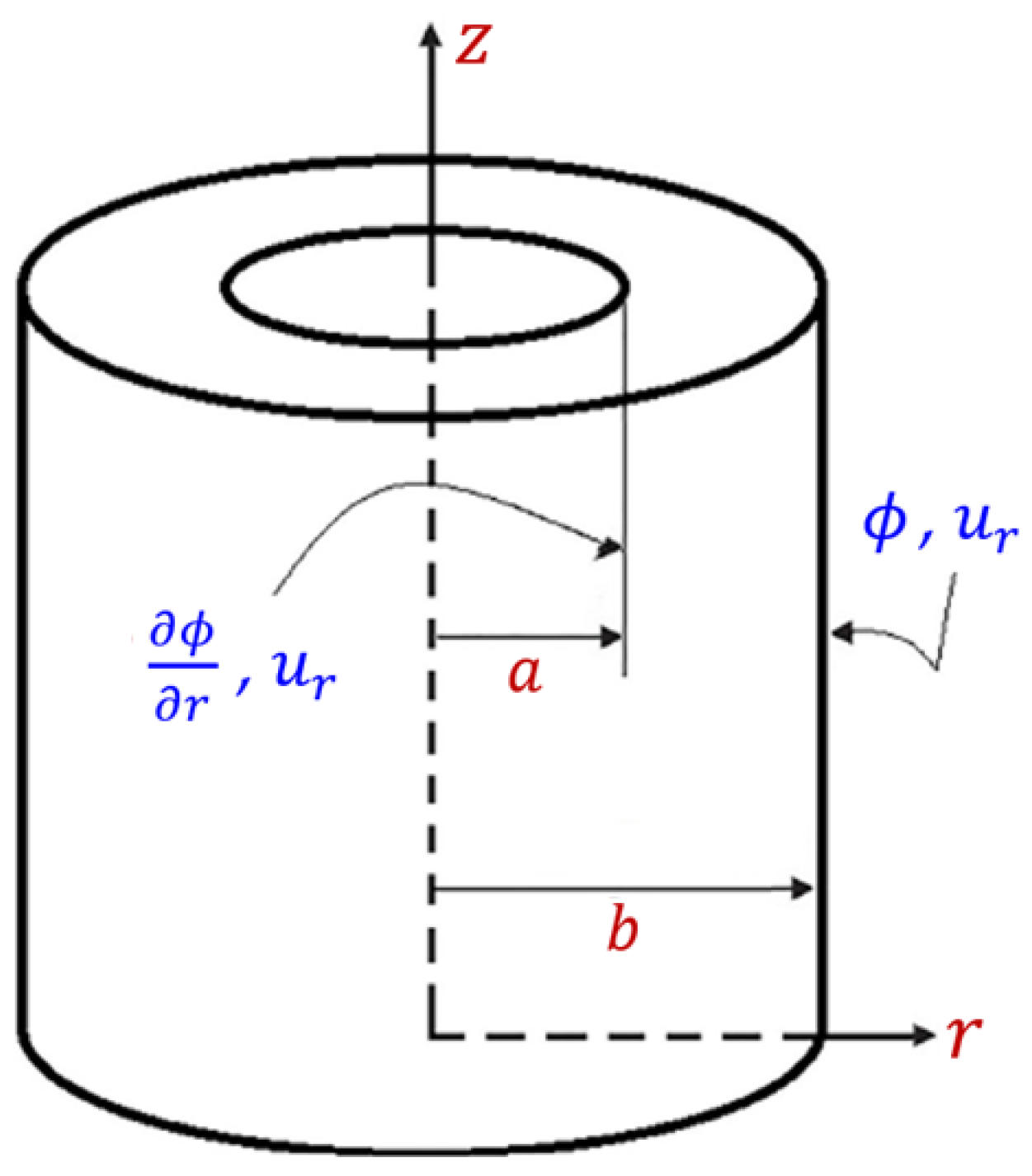
The constitutive equations and field equations for a homogeneous, isotropic, and perfectly conducting elastic circular cylinder (Figure 1) under the fractional-order theory of generalized thermoelasticity can be written as:

2.1. Time-Fractional Heat Conduction Equation

The generalized heat conduction equation with fractional derivative heat transfer, extended by the refined form of Lord and Shulman [39,43,44] (F-LS (r)) theory, is

$${\mathcal{D}}_1\left[\kappa \left(\theta \right){\mathcal{D}}_0\left(\theta \right)\right]=\mathcal{D}\left(\rho c_{\vartheta }{\displaystyle \frac{\partial \theta }{\partial t}}+\gamma T_0{\displaystyle \frac{\partial \epsilon }{\partial t}}-Q\right),$$

(1)

where $\kappa$ represents the variable thermal conductivity, $\rho$ is the material density of the circular cylinder, $c_{\vartheta }$ denotes the specific heat at fixed strain, $Q(r,t)$ is the heat source, $\epsilon =\nabla ·\stackrel{⃑}{u}$ is dilatation in which $\stackrel{⃑}{u}\equiv \left(u,0,0\right)$ is the displacement vector, and $\gamma =\left(3\lambda +2\mu \right)\alpha$ is the coupling parameter in which $\lambda$, $\mu$ denote Lamé’s moduli and $\alpha$ denotes the linear parameter of thermal expansion. Also, $\theta =T-T_0$ represents the temperature increment wherein $T_0$ denotes the reference temperature, $T(r,t)$ is the absolute temperature, ${\mathcal{D}}_0$ and ${\mathcal{D}}_1$ represent the two differential parameters

$${\mathcal{D}}_0={\displaystyle \frac{\partial }{\partial r}}, {\mathcal{D}}_1={\displaystyle \frac{\partial }{\partial r}}+{\displaystyle \frac{1}{r}}, {\mathcal{D}}_1{\mathcal{D}}_0={\nabla }^2,$$

(2)

in which ${\nabla }^2$ is the Laplacian in the cylindrical coordinates, and $\mathcal{D}$ is the differential parameter

$$\mathcal{D}=1+{\sum }_{n=1}^N{\displaystyle \frac{{\tau }^{n+\beta }}{\left(n+\beta \right)!}}{\displaystyle \frac{{\partial }^{n+\beta }}{\partial t^{n+\beta }}}, N\ge 1,$$

(3)

where $\tau$ is the first relaxation time and $\beta$ is the fractional-order parameter ($0<\beta \le 1$). The simple heat conduction equation with fractional derivative (FD (s)) heat transfer in the context of Equation (1) can be reduced to (neglecting the summation)

$${\mathcal{D}}_1\left[\kappa \left(\theta \right){\mathcal{D}}_0\left(\theta \right)\right]=\left(1+{\displaystyle \frac{{\tau }^{\beta }}{\alpha !}}{\displaystyle \frac{{\partial }^{\beta }}{\partial t^{\beta }}}\right)\left[\rho c_{\vartheta }{\displaystyle \frac{\partial \theta }{\partial t}}+\gamma T_0{\displaystyle \frac{\partial \epsilon }{\partial t}}-Q\right], 0<\beta \le 1.$$

(4)

It is clear that the case of $\beta =1$ in Equation (4) represents the simple Lord and Shulman (LS (s)) theory [44]

$${\mathcal{D}}_1\left[\kappa \left(\theta \right){\mathcal{D}}_0\left(\theta \right)\right]=\left(1+\tau {\displaystyle \frac{\partial }{\partial t}}\right)\left[\rho c_{\vartheta }{\displaystyle \frac{\partial \theta }{\partial t}}+\gamma T_0{\displaystyle \frac{\partial \epsilon }{\partial t}}-Q\right],$$

(5)

while the case of omitting $\beta$ represents the classical thermoelasticity (CTE) theory [45]

$${\mathcal{D}}_1\left[\kappa \left(\theta \right){\mathcal{D}}_0\left(\theta \right)\right]=\rho c_{\vartheta }{\displaystyle \frac{\partial \theta }{\partial t}}+\gamma T_0{\displaystyle \frac{\partial \epsilon }{\partial t}}-Q.$$

(6)

Also, in the case of $N=1$, one can obtain the generalized heat conduction equation with fractional derivative heat transfer in the simplest fractional-order form of Lord and Shulman (F-LS (s)) theory in the form

$${\mathcal{D}}_1\left[\kappa \left(\theta \right){\mathcal{D}}_0\left(\theta \right)\right]=\left(1+{\displaystyle \frac{{\tau }^{1+\beta }}{\left(1+\beta \right)!}}{\displaystyle \frac{{\partial }^{1+\beta }}{\partial t^{1+\beta }}}\right)\left(\rho c_{\vartheta }{\displaystyle \frac{\partial \theta }{\partial t}}+\gamma T_0{\displaystyle \frac{\partial \epsilon }{\partial t}}-Q\right), 0<\beta <1.$$

(7)

Setting $\beta \to 0$ in the above equation, one can return to the LS (s) theory as in Equation (5). However, by setting $\beta \to 0$ in Equation (1) with the aid of Equation (3), one can obtain the refined Lord and Shulman (LS (r)) theory in the form

$${\mathcal{D}}_1\left[\kappa \left(\theta \right){\mathcal{D}}_0\left(\theta \right)\right]=\left(1+{\sum }_{n=1}^N{\displaystyle \frac{{\tau }^n}{n!}}{\displaystyle \frac{{\partial }^n}{\partial t^n}}\right)\left(\rho c_{\vartheta }{\displaystyle \frac{\partial \theta }{\partial t}}+\gamma T_0{\displaystyle \frac{\partial \epsilon }{\partial t}}-Q\right), N\ge 1.$$

(8)

2.2. Equation of Motion

The equation of motion may be expressed as

$${\displaystyle \frac{\partial {\sigma }_r}{\partial r}}+{\displaystyle \frac{{\sigma }_r-{\sigma }_{\vartheta }}{r}}+F_r=\rho {\displaystyle \frac{{\partial }^{2}u}{\partial t^2}},$$

(9)

where ${\sigma }_r$ and ${\sigma }_{\vartheta }$ are the radial and circumferential stresses, $F_r$ are Lorentz forces of the cylinder, and ($r$, $\vartheta$, $z$) are the cylindrical coordinate system.

2.3. Constitutive and Cauchy Relations

The constitutive equations of the cylinder are given by

$${\sigma }_r=\left(\lambda +2\mu \right){\mathcal{D}}_0{u}_r+\lambda {\displaystyle \frac{u}{r}}-\gamma \theta , {\sigma }_{\vartheta }=\left(\lambda +2\mu \right){\displaystyle \frac{u_r}{r}}+\lambda {\mathcal{D}}_{0}u-\gamma \theta .$$

(10)

The relationship between the radial displacement $u$ and strains is independent of the thickness and density of the circular cylinder. It can be written as

$${\epsilon }_r={\displaystyle \frac{\partial u}{\partial r}}, {\epsilon }_{\vartheta }={\displaystyle \frac{u}{r}}, {\epsilon }_z=0,$$

(11)

where ${\epsilon }_r$, ${\epsilon }_{\vartheta }$, ${\epsilon }_z$ are the radial, circumferential, and axial strains, respectively, and the dilatation $\epsilon$ is given by

$$\epsilon ={\epsilon }_r+{\epsilon }_{\vartheta }={\displaystyle \frac{1}{r}}{\displaystyle \frac{\partial }{\partial r}}\left(r u_r\right)={\mathcal{D}}_1{u}_r.$$

(12)

2.4. Variable Thermal Conductivity

To deal with the variable thermal conductivity, we will use the temperature-mapping

$$\varphi ={\displaystyle \frac{1}{{\kappa }_0}}{\int }_0^{\theta }\kappa \left({\theta }^{\prime }\right)\mathrm{d}{\theta }^{\prime }.$$

(13)

Differentiating the above mapping with respect to time, one obtains

$${\kappa }_0{\displaystyle \frac{\partial \varphi }{\partial t}}=\kappa \left(\theta \right){\displaystyle \frac{\partial \theta }{\partial t}}.$$

(14)

Now, apply the operator ${\mathcal{D}}_0$ on both sides of Equation (13) yields

$${\kappa }_0{\mathcal{D}}_0\left(\varphi \right)=\kappa \left(\theta \right){\mathcal{D}}_0\left(\theta \right).$$

(15)

Next, apply the operator ${\mathcal{D}}_1$ on both sides of Equation (15) yields

$${\kappa }_0{\nabla }^2\varphi ={\mathcal{D}}_1\left[\kappa \left(\theta \right){\mathcal{D}}_0\left(\theta \right)\right].$$

(16)

So the heat conduction equation that appeared in Equation (1), without the heat source, becomes

$${\nabla }^2\varphi =\mathcal{D}\left({\displaystyle \frac{1}{\eta }}{\displaystyle \frac{\partial \varphi }{\partial t}}+{\displaystyle \frac{\gamma T_0}{{\kappa }_0}}{\displaystyle \frac{\partial \epsilon }{\partial t}}\right),$$

(17)

where $\eta =\kappa \left(\theta \right)/\left(\rho c_{\vartheta }\right)$.

A common linear approximation of thermal conductivity is

$$\kappa \left(\theta \right)={\kappa }_0\left(1+{\kappa }_1\theta \right),$$

(18)

where ${\kappa }_0$ is the reference conductivity and ${\kappa }_1$ is a material parameter. From Equations (14) and (16), one obtains

$$\varphi =\theta +{\displaystyle \frac{{\kappa }_1}{2}}{\theta }^2, {\mathcal{D}}_0\left(\varphi \right)=\left(1+{\kappa }_1\theta \right){\mathcal{D}}_0\left(\theta \right).$$

(19)

The first part of Equation (19) yields

$$\theta ={\displaystyle \frac{-1+\sqrt{1+2{\kappa }_1\varphi }}{{\kappa }_1}}.$$

(20)

2.5. Initial and Boundary Conditions

Let us consider some relations to describe the imposed initial and boundary conditions of the problem. On both internal and external surfaces, the circular cylinder is clamped. That is

$${\left.u_r\left(r,t\right)\right|}_{r=a}={\left.u_r\left(r,t\right)\right|}_{r=b}=0.$$

(21)

The inner surface is isolated while the outer surface is subjected to an exponential decay of temperature-mapping over time. That is

$${\left.{\displaystyle \frac{\partial \varphi \left(r,t\right)}{\partial r}}\right|}_{r=a}=0, {\left.\varphi \left(r,t\right)\right|}_{r=b}={\varphi }_0{\displaystyle \frac{t^2}{16t_0^2}}{\mathrm{e}}^{-t/t_0},$$

(22)

where ${\varphi }_0$ and $t_0$ are constants, ${\mathrm{e}}^{-t/t_0}$ is the exponential decay term in which $t_0$ is the exponential decay time. These conditions simulate a thermally driven, mechanically restrained viscoelastic medium under transient heating. Concerning the initial conditions, one can assume the following equations that describe the initial conditions

$$\varphi \left(r,0\right)={\displaystyle \frac{{\partial }^n}{\partial t^n}}\varphi \left(r,0\right)=\psi \left(r,0\right)={\displaystyle \frac{{\partial }^n}{\partial t^n}}\psi \left(r,0\right)=0, n=1, 2, 3, \dots .$$

(23)

3. Solution to the Problem

3.1. Laplace Transform

Let us apply the well-known Laplace transform given by

$$\mathcal{L}\left\{f\left(r,t\right)\right\}=\overline{f}\left(r,s\right)={\int }_0^{\mathrm{\infty }}f\left(r,t\right){\mathrm{e}}^{-st}\mathrm{d}t.$$

(24)

3.2. Dimensionless Physical Variables

The dimensionless variables take the following form

$$\begin{gathered} \left\{r^{\prime },u^{\prime }\right\}={\displaystyle \frac{c_0}{\eta }}\left\{r,u\right\}, \left\{t^{\prime },{\tau }^{\prime },t_0\right\}={\displaystyle \frac{c_0^2}{\eta }}\left\{t,\tau \right\}, \left\{{\theta }^{\prime },{\varphi }^{\prime }\right\}={\displaystyle \frac{1}{T_0}}\left\{\theta ,\varphi \right\}, \\ {\sigma }_j^{\prime }={\displaystyle \frac{{\sigma }_j}{\lambda +2\mu }}, {\kappa }_1^{\prime }=T_0{\kappa }_1, t_0^{\prime }={\displaystyle \frac{\eta }{c_0^2}}{t}_0, c_0^2={\displaystyle \frac{\lambda +2\mu }{\rho }}. \end{gathered}$$

(25)

In addition, and without losing any generality, we can approximate the thermal conductivity as $\kappa \left(\theta \right)\approx \kappa \left(T_0\right)$ for linearity which is constant depending on the reference temperature $T_0$. Then, using Equation (31), the above expressions and equations become (omitting the prime)

$${\overline{\sigma }}_r=\left({\mathcal{D}}_0+{\displaystyle \frac{c_1}{r}}\right){\overline{u}}_r-c_2\overline{\theta }, {\overline{\sigma }}_{\vartheta }=\left(c_1{\mathcal{D}}_0+{\displaystyle \frac{1}{r}}\right){\overline{u}}_r-c_2\overline{\theta },$$

(26)

$$\left({\mathcal{D}}_0{\mathcal{D}}_1+2c_3\right){\overline{u}}_r-2c_4{\mathcal{D}}_0\overline{\varphi }=0,$$

(27)

$$\left({\mathcal{D}}_1{\mathcal{D}}_0+2c_5\right)\overline{\varphi }+c_6{\mathcal{D}}_1{\overline{u}}_r=0,$$

(28)

where

$$c_1={\displaystyle \frac{\lambda }{\lambda +2\mu }}, c_2={\displaystyle \frac{\gamma T_0}{\lambda +2\mu }}, c_3=-{\displaystyle \frac{s^2}{2}}, c_4={\displaystyle \frac{\gamma T_0}{2\rho c_0^2\left(1+{\kappa }_1\right)}}, c_5=-{\displaystyle \frac{\varpi }{2}}, c_6=-{\displaystyle \frac{\gamma \varpi \left(1+{\kappa }_1\right)}{\rho c_{\nu }}}.$$

(29)

The parameter $\varpi$ will be given according to the theory used. That is

The classical thermoelasticity theory (CTE):

$$\varpi =s.$$

(30)

The simple Lord and Shulman thermoelasticity theory (LS (s)):

$$\varpi =s\left(1+\tau s\right).$$

(31)

The refined Lord and Shulman thermoelasticity theory (LS (r)):

$$\varpi =s\left(1+{\sum }_{n=1}^N{\displaystyle \frac{{\tau }^n}{n!}}{s}^n\right).$$

(32)

For the present fractional-order theories:

If $\beta >0$, $m=\left[\beta \right]+1$, and if $h\left(t\right)$, $h^{\prime }\left(t\right)$, $h^{″}\left(t\right)$, …, $h^{\left(m-1\right)}\left(t\right)$ are continuous on the interval $[0,\mathrm{\infty })$ and of exponential order, while ${\displaystyle \frac{{\partial }^{\beta }}{\partial t^{\beta }}}h\left(t\right)$ with order $\alpha$ is piecewise continuous on the interval $[0,\mathrm{\infty })$, then the Laplace transform of Caputo fractional derivative of $h\left(t\right)$ is defined as

$$\mathcal{L}\left\{{\displaystyle \frac{{\partial }^{\beta }}{\partial t^{\beta }}}h\left(t\right)\right\}=s^{\beta }\mathcal{L}\left\{h\left(t\right)\right\}-{\sum }_{k=0}^{m-1}{s}^{\beta -k-1}{h}^{\left(k\right)}(0).$$

(33)

Because of the above equation and the initial conditions appearing in Equation (25), we obtain the parameter $\varpi$ according to the fraction theory used in the following form:

The simple fractional derivative thermoelasticity theory (FD (s)):

$$\varpi =s\left(1+{\displaystyle \frac{{\tau }^{\beta }}{\beta !}}{s}^{\beta }\right).$$

(34)

The simple fractional order of the Lord and Shulman thermoelasticity theory (F-LS (s)):

$$\varpi =s\left(1+{\displaystyle \frac{{\tau }^{1+\beta }}{\left(1+\beta \right)!}}{s}^{1+\beta }\right).$$

(35)

The refined Lord and Shulman thermoelasticity theory (LS (r)):

$$\varpi =s\left(1+{\sum }_{n=1}^N{\displaystyle \frac{{\tau }^{n+\beta }}{\left(n+\beta \right)!}}{s}^{n+\beta }\right), N>1.$$

(36)

3.3. Bessel’s Functions

The solution of the physical quantities can be decomposed in the Laplace domain in the following form:

$$\overline{\varphi }\left(r\right)={\sum }_{j=1}^2\left[A_j{J}_0\left({\xi }_{j}r\right)+B_j{Y}_0\left({\xi }_{j}r\right)\right],$$

(37)

$${\overline{u}}_r\left(r\right)={\sum }_{j=1}^2{\zeta }_j\left[A_j{J}_1\left({\xi }_{j}r\right)+B_j{Y}_1\left({\xi }_{j}r\right)\right],$$

(38)

where $A_j$ and $B_j$ ($j=1,2$) are the integration constants, $J_0\left(R\right)$, $J_1\left(R\right)$ are Bessel’s functions of the first kind of orders 0 and 1; $Y_0\left(R\right)$, $Y_1\left(R\right)$ are Bessel’s functions of the second kind of orders 0 and 1, and

$$\begin{gathered} {\xi }_1^2,{\xi }_2^2=c_3+c_5+c_4{c}_6\mp {\xi }_0, {\xi }_0^2={\left(c_3+c_5+c_4{c}_6\right)}^2-4c_3{c}_5, \\ {\zeta }_1={\displaystyle \frac{{\xi }_1\left(c_3-c_5-c_4{c}_6-{\xi }_0\right)}{2c_3{c}_6}}, {\zeta }_2={\displaystyle \frac{{\xi }_2\left(c_3-c_5-c_4{c}_6+{\xi }_0\right)}{2c_3{c}_6}}. \end{gathered}$$

(39)

The temperature of the cylinder in the Laplace domain may be obtained in terms of $\overline{\varphi }\left(r\right)$ in the form

$$\overline{\theta }\left(r\right)={\displaystyle \frac{1}{{\kappa }_1}}\left[{\left(1+2{\kappa }_1{\sum }_{j=1}^2\left[A_j{J}_0\left({\xi }_{j}r\right)+B_j{Y}_0\left({\xi }_{j}r\right)\right]\right)}^{1/2}-1\right].$$

(40)

The dilatation and radial and hoop stresses may be obtained in the Laplace domain in the form

$$\overline{\epsilon }\left(r\right)={\sum }_{j=1}^2{\xi }_j{\zeta }_j\left[A_j{J}_0\left({\xi }_{j}r\right)+B_j{Y}_0\left({\xi }_{j}r\right)\right],$$

(41)

$${\overline{\sigma }}_r\left(r\right)={\sum }_{j=1}^2\left[A_j{\breve{J}}_r\left({\xi }_{j}r\right)+B_j{\breve{Y}}_r\left({\xi }_{j}r\right)\right]-c_2\overline{\theta }\left(r\right),$$

(42)

$${\overline{\sigma }}_{\vartheta }\left(r\right)={\sum }_{j=1}^2\left[A_j{\breve{J}}_{\vartheta }\left({\xi }_{j}r\right)+B_j{\breve{Y}}_{\vartheta }\left({\xi }_{j}r\right)\right]-c_2\overline{\theta }\left(r\right),$$

(43)

where

$$\begin{array}{c}{\breve{J}}_r\left({\xi }_{j}r\right)={\zeta }_j\left[{\xi }_j{J}_0\left({\xi }_{j}r\right)+{\displaystyle \frac{c_1-1}{r}}{J}_1\left({\xi }_{j}r\right)\right],\\ {\breve{Y}}_r\left({\xi }_{j}r\right)={\zeta }_j\left[{\xi }_j{Y}_0\left({\xi }_{j}r\right)+{\displaystyle \frac{c_1-1}{r}}{Y}_1\left({\xi }_{j}r\right)\right],\\ {\breve{J}}_{\vartheta }\left({\xi }_{j}r\right)={\zeta }_j\left[c_1{\xi }_j{J}_0\left({\xi }_{j}r\right)-{\displaystyle \frac{c_1-1}{r}}{J}_1\left({\xi }_{j}r\right)\right],\\ {\breve{Y}}_{\vartheta }\left({\xi }_{j}r\right)={\zeta }_j\left[c_1{\xi }_j{Y}_0\left({\xi }_{j}r\right)-{\displaystyle \frac{c_1-1}{r}}{Y}_1\left({\xi }_{j}r\right)\right].\end{array}$$

(44)

3.4. Applications

The boundary conditions (21) and (22) in the Laplace transform domain can be obtained as

$${\displaystyle \frac{\mathrm{d}\overline{\varphi }\left(a,s\right)}{\mathrm{d}r}}=0, \overline{\varphi }\left(b,s\right)=\overline{G}\left(s\right)={\displaystyle \frac{{\varphi }_0\left(1-{\mathrm{e}}^{-t_{0}p}\right)}{t_0{p}^2}}, {\overline{u}}_r\left(a,s\right)={\overline{u}}_r\left(b,s\right)=0.$$

(45)

Using the above conditions, the parameters $A_j$, $j=\mathrm{1,2},2,\dots ,5$ will be obtained from the following simultaneous equations

$${\sum }_{j=1}^2{\zeta }_j\left[A_j{J}_1\left({\xi }_{j}a\right)+B_j{Y}_1\left({\xi }_{j}a\right)\right]=0,$$

(46)

$${\sum }_{j=1}^2{\zeta }_j\left[A_j{J}_1\left({\xi }_{j}b\right)+B_j{Y}_1\left({\xi }_{j}b\right)\right]=0,$$

(47)

$${\sum }_{j=1}^2{\xi }_j\left[A_j{J}_1\left({\xi }_{j}a\right)+B_j{Y}_1\left({\xi }_{j}a\right)\right]=0,$$

(48)

$${\sum }_{j=1}^2\left[A_j{J}_0\left({\xi }_{j}b\right)+B_j{Y}_0\left({\xi }_{j}b\right)\right]=\overline{G}\left(s\right).$$

(49)

Solving the above system of simultaneous equations gives the parameters $A_j$ and $B_j$. With the aid of these parameters, one can determine all field quantities of the circular cylinder in the Laplace domain.

4. Numerical Results and Discussion

To invert the Laplace transform numerically, we can use the Riemann sum approximation method [46,47]. For a fixed $r$, the function $\overline{f}\left(r,s\right)$ represents the Laplace transform of $f\left(r,t\right)$. The inverse Laplace transform $f\left(r,t\right)$ can be approximated by

$$f\left(r,t\right)={\displaystyle \frac{{\mathrm{e}}^{ct}}{t}}\left[{\displaystyle \frac{1}{2}}\overline{f}\left(r,c\right)+\mathrm{R}\mathrm{e}\left({\sum }_{m=1}^M{\left(-1\right)}^m\overline{f}\left(r,c+{\displaystyle \frac{\mathrm{i}m\pi }{t}}\right)\right)\right],$$

(50)

where $c$ is an arbitrary constant (optimally chosen such that $ct\approx 4.7$ for faster convergence [46,47]), $\mathrm{R}\mathrm{e}$ denotes the real part, $\mathcal{i}=\sqrt{-1}$ and $M$ is a sufficiently large integer for accuracy.

Figure 2, Figure 3, Figure 4, Figure 5, Figure 6, Figure 7, Figure 8, Figure 9, Figure 10, Figure 11, Figure 12, Figure 13, Figure 14, Figure 15, Figure 16, Figure 17, Figure 18, Figure 19, Figure 20 and Figure 21 show the field variables along the radial direction of the circular cylinder employing the refined fractional order of the Lord and Shulman thermoelasticity theory (LS (r)), the simple fractional order of the Lord and Shulman thermoelasticity theory (F-LS (s)), the simple fractional derivative thermoelasticity theory (FD (s)), the refined Lord and Shulman thermoelasticity theory (LS (r)), the simple Lord and Shulman thermoelasticity theory (LS (s)), and the classical thermoelasticity theory (CTE).

In the recommendations, a series of applications will be introduced to ensure the impact of various change models. The properties of the material required in numerical calculations are provided by applying the copper material constants as

$$\begin{array}{c}\lambda =7.76\times {10}^{10}\left(\mathrm{k}\mathrm{g} {\mathrm{m}}^{-1} {\mathrm{s}}^{-2}\right), \mu =3.86\times {10}^{10}\left(\mathrm{k}\mathrm{g} {\mathrm{m}}^{-1} {\mathrm{s}}^{-2}\right),\\ \rho =8954\left(\mathrm{k}\mathrm{g} {\mathrm{m}}^{-3}\right), c_{\vartheta }=383.1\left(\mathrm{J} {\mathrm{k}\mathrm{g}}^{-1} {\mathrm{K}}^{-1}\right), \alpha =1.78\times {10}^{-5}\left({\mathrm{K}}^{-1}\right),\\ \kappa =386\left(\mathrm{W} {\mathrm{m}}^{-1} {\mathrm{K}}^{-1}\right), T_0=293 \mathrm{K}.\end{array}$$

(51)

For convenience, the real estimations of the thermoelastic variables have been embraced to represent the numerical outcomes. These outcomes are gained for $t=0.3$, ${\tau }_q=0.01$, and ${\varphi }_0={10}^2$. The values of some parameters are fixed, except otherwise stated, as $t_0=0.1$, ${\kappa }_1=1.1$, and $\beta =0.3$. Results for all variables: the temperature-mapping $\varphi \left(r,t\right)$; the temperature $\theta \left(r,t\right)$; the radial displacement $\widehat{u}\equiv {10}^3\times u\left(r,t\right)$; the dilatation $\widehat{\epsilon }\equiv {10}^2\times \epsilon \left(r,t\right)$; the radial stress ${\widehat{\sigma }}_r\equiv {10}^2\times {\sigma }_r\left(r,t\right)$; and the hoop stress ${\widehat{\sigma }}_{\vartheta }\equiv {10}^2\times {\sigma }_{\vartheta }\left(r,t\right)$ due to the various theories being considered. The outcomes are illustrated in Figure 2, Figure 3, Figure 4, Figure 5, Figure 6, Figure 7, Figure 8, Figure 9, Figure 10, Figure 11, Figure 12, Figure 13, Figure 14, Figure 15, Figure 16, Figure 17, Figure 18, Figure 19, Figure 20 and Figure 21.

4.1. Comparison Between Various Theories

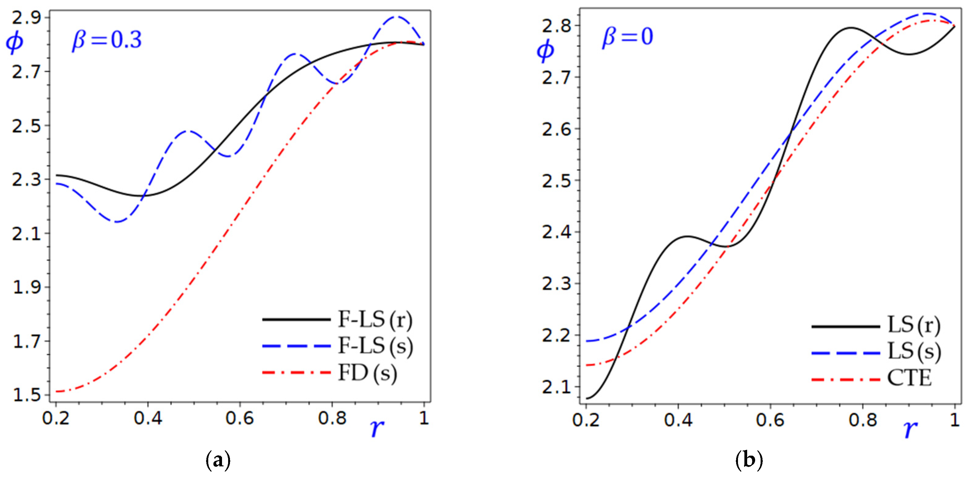
The graphs in Figure 2 compare the temperature-mapping $\varphi$ for the circular cylinder under two scenarios: with ($\beta =0.3$) and without ($\beta =0$) the fraction parameter. The curves in Figure 2a show how $\varphi$ varies with $r$ for $\beta =0.3$, with F-LS (r) exhibiting the highest values. However, the curves in Figure 2b are closer together compared to Figure 2a, indicating less variation in $\varphi$ when $\beta =0$. The inclusion of $\beta$ in graph (a) leads to a wider range of $\varphi$ values and distinct separation between theories, while its absence in graph (b) results in more clustered curves. All theories (F-LS, FD, LS, CTE) are used to investigate the temperature-mapping distribution, with differences in their predictions highlighted.

Figure 2. The temperature-mapping $\varphi$ of the circular cylinder with and without the fraction parameter: (a) $\beta =0.3$; (b) $\beta =0$.

Figure 2. The temperature-mapping $\varphi$ of the circular cylinder with and without the fraction parameter: (a) $\beta =0.3$; (b) $\beta =0$.

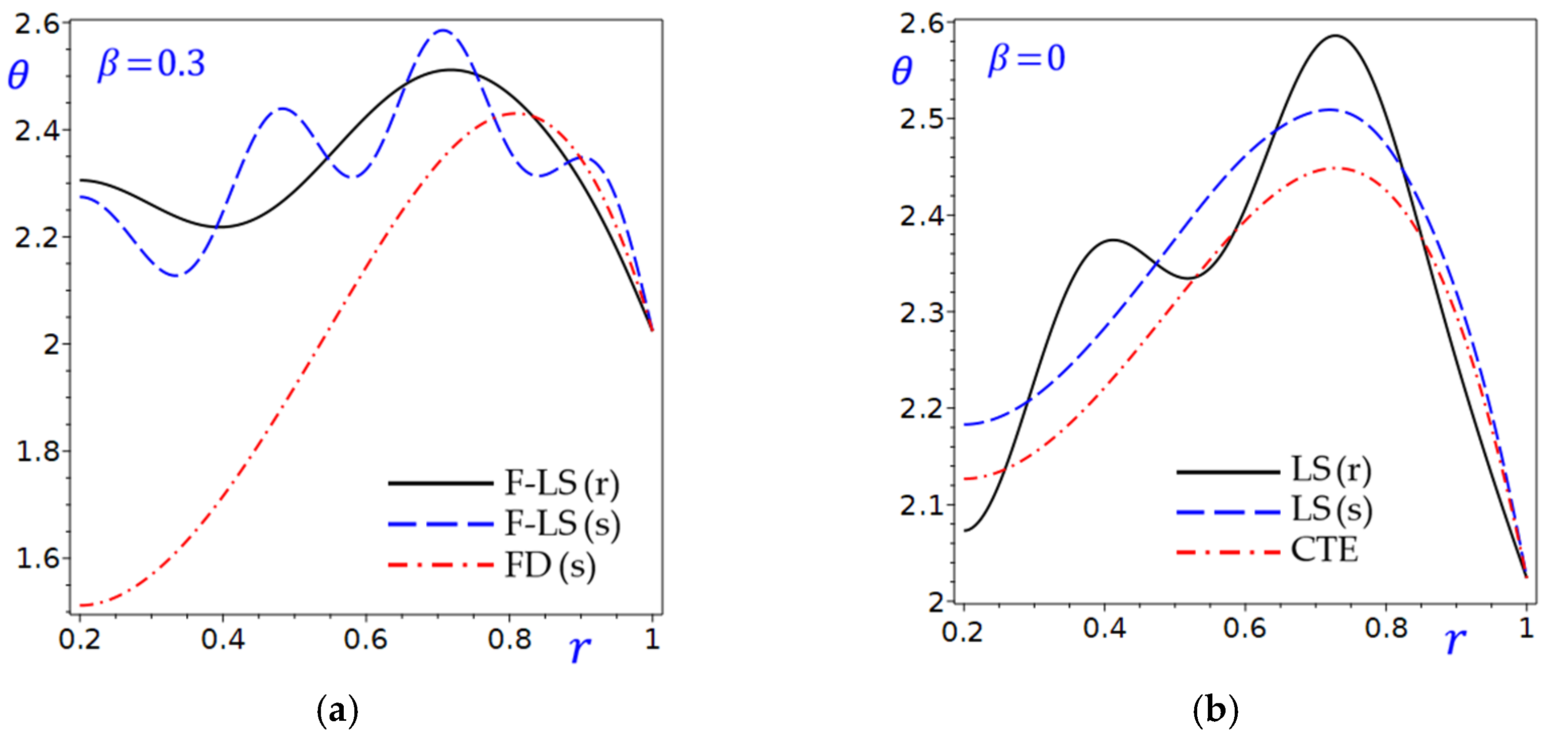
Figure 3 depicts the relationship between the temperature $\theta$ and $r$ on the horizontal axis under different conditions. In Figure 3a, all curves show an increasing trend in $\theta$ as $r$ increases from 0.2 to 0.8. The curve of refined fractional F-LS (r) theory starts highest ($\theta \approx 2.3$ at $r=0.2$) and decreases sharply. The curves of the simple fraction F-LS (s) and FD (s) theories start lower and decline more gradually. The gap between F-LS (r) and the other two curves narrows as $r$ increases. In Figure 3b, all curves show an increasing trend in $\theta$ as $r$ increases from 0.2 to 0.75. The curve of $\theta$ due to the refined LS (r) theory starts lowest ($\theta \approx 2.07$ at $r=0.2$) and increases rapidly. The temperature due to the LS (s) and CTE theories starts higher and declines more gradually. The gap between $\theta$ due to the refined LS (r) theory and the other two theories narrows as $r$ increases. In both plots, $\theta$ is no longer increasing and decreasing again, with its maximum occurring at $0.6\le r\le 0.8$. The rate of decrease is steeper for curves due to the refined theories compared to the simple or other theories. Figure 3a ($\beta =0.3$) shows higher initial $\theta$ values compared to Figure 3b with $\beta =0$, suggesting $\beta$ influences the baseline $\theta$. The refined F-LS (r) or LS (r) theories consistently yield higher $\theta$ values at lower $r$ but converge with other theories as $r$ increases. The CTE and FD (s) theories exhibit more stable or gradual declines in temperature.

Figure 3. The temperature $\theta$ of the circular cylinder with and without the fraction parameter: (a) $\beta =0.3$; (b) $\beta =0$.

Figure 3. The temperature $\theta$ of the circular cylinder with and without the fraction parameter: (a) $\beta =0.3$; (b) $\beta =0$.

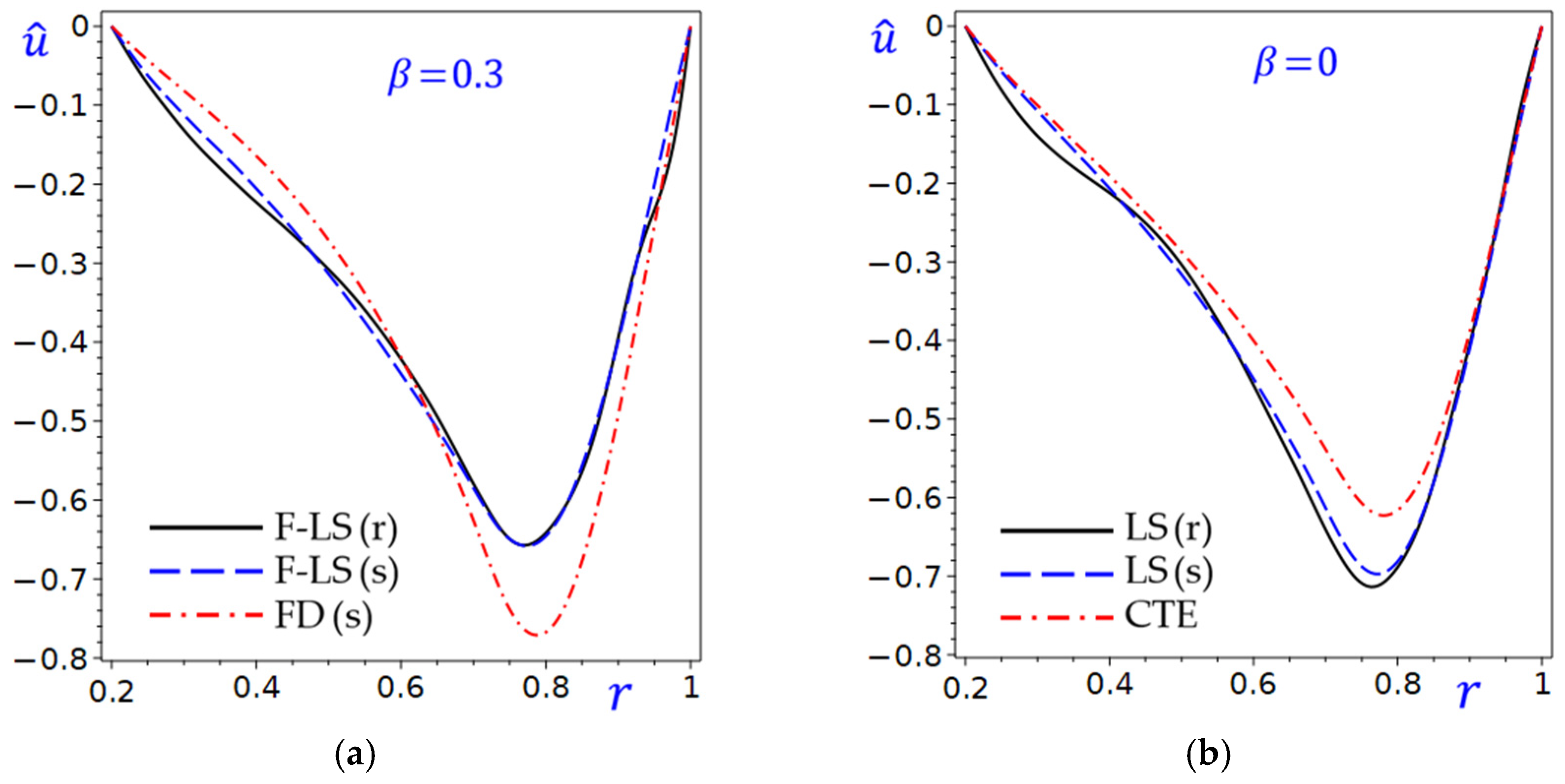
Figure 4 shows the radial displacement $\widehat{u}$ of the circular cylinder with and without the fraction parameter (a) $\beta =0.3$ (b) $\beta =0$. In Figure 4a, the curves show how the radial displacement changes along the radial direction of the cylinder with $\beta =0.3$. The fractional F-LS and FD theories are compared, with one likely being a benchmark. The F-LS (r) and FD (s) theories may converge or diverge as $r$ increases. The curves in Figure 4b may show how the generalized and classical theories perform under $\beta =0$, with the CTE theory potentially serving as a theoretical or ideal case. The LS (r) and CTE theories might represent bounds or benchmarks for LS (s) theory. Generally, both plots explore the effect of $r$, with $\beta$ fixed at 0.3 in Figure 4a and 0 in Figure 4b. This suggests $\beta$ modulates the radial displacement $\widehat{u}$ of the cylinder’s behavior.

Figure 4. The radial displacement $\widehat{u}$ of the circular cylinder with and without the fraction parameter: (a) $\beta =0.3$; (b) $\beta =0$.

Figure 4. The radial displacement $\widehat{u}$ of the circular cylinder with and without the fraction parameter: (a) $\beta =0.3$; (b) $\beta =0$.

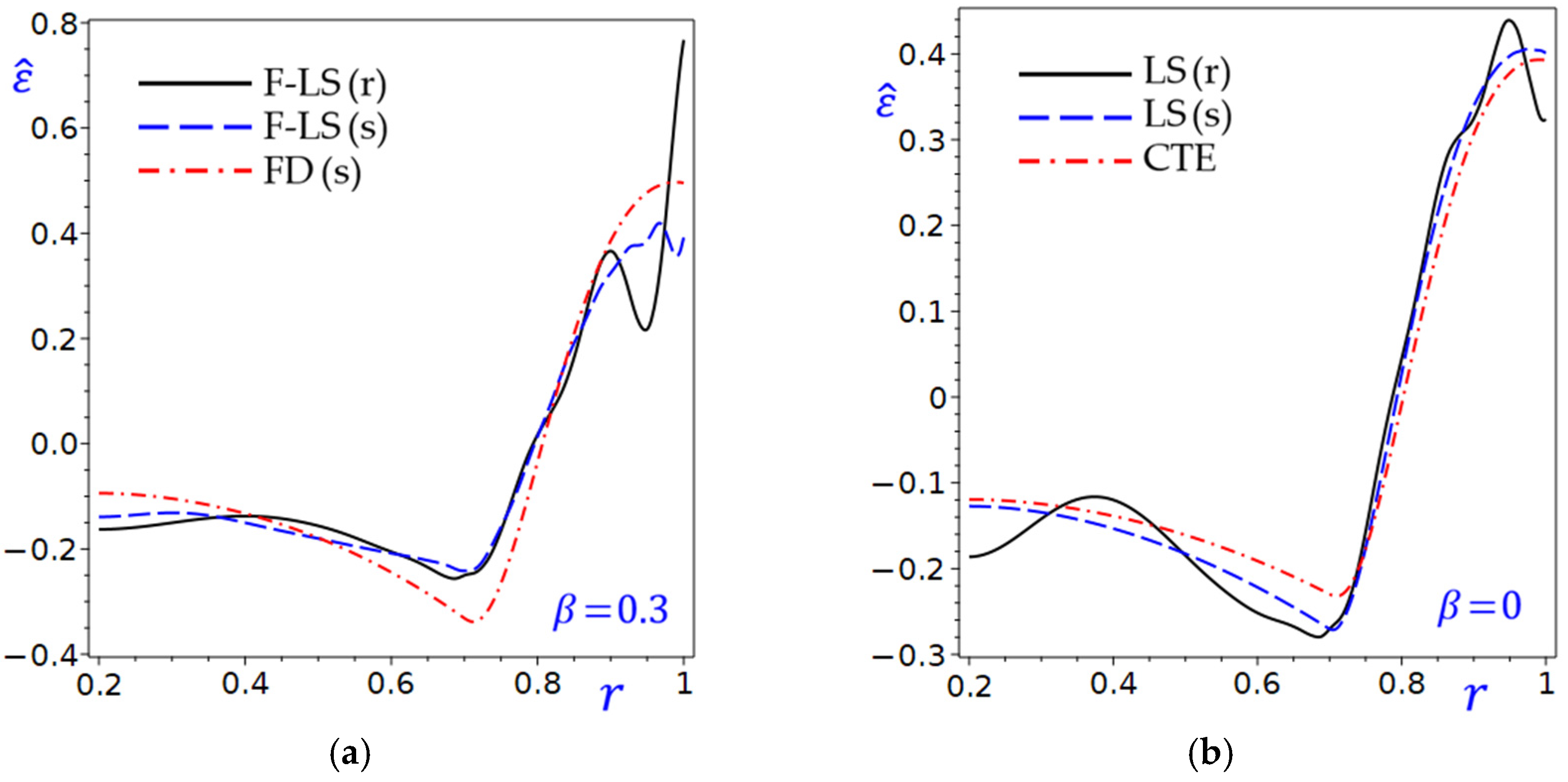
Figure 5 shows the dilatation $\widehat{\epsilon }$ of the circular cylinder with ($\beta =0.3$) and without ($\beta =0$) the fraction parameter. All curves in Figure 5a start near $\widehat{\epsilon }=-0.1$ at $r=0.2$. As $r$ increases, $\widehat{\epsilon }$ rises sharply for the fractional F-LS (r) and F-LS (s) theories, peaking around $r=0.4$ before declining. The FD (s) theory shows a more gradual increase, peaking later (around $r=0.7$) and remaining positive for higher $r$ values. The plot highlights how $\widehat{\epsilon }$ is sensitive to $r$, with theory-dependent variations. Also, all curves in Figure 5b start near $\widehat{\epsilon }=-0.1$ at $r=0.2$. The LS (s) and CTE theories show similar trends, declining to a peak around $r=0.7$ before rising. The plot demonstrates how $\beta =0$ leads to smaller $\widehat{\epsilon }$ magnitudes compared to $\beta =0.3$ as in Figure 5a. In general, both plots show that $\widehat{\epsilon }$ is highly dependent on $r$, with peaks at $r=0.7$. Different theories yield varying $\widehat{\epsilon }$ trends, highlighting the importance of theory selection in analysis. The contrast between $\beta =0.3$ in Figure 5a and $\beta =0$ in Figure 5b suggests that $\beta$ influences the magnitude and shape of $\widehat{\epsilon }$ curves.

Figure 5. The dilatation $\widehat{\epsilon }$ of the circular cylinder with and without the fraction parameter: (a) $\beta =0.3$; (b) $\beta =0$.

Figure 5. The dilatation $\widehat{\epsilon }$ of the circular cylinder with and without the fraction parameter: (a) $\beta =0.3$; (b) $\beta =0$.

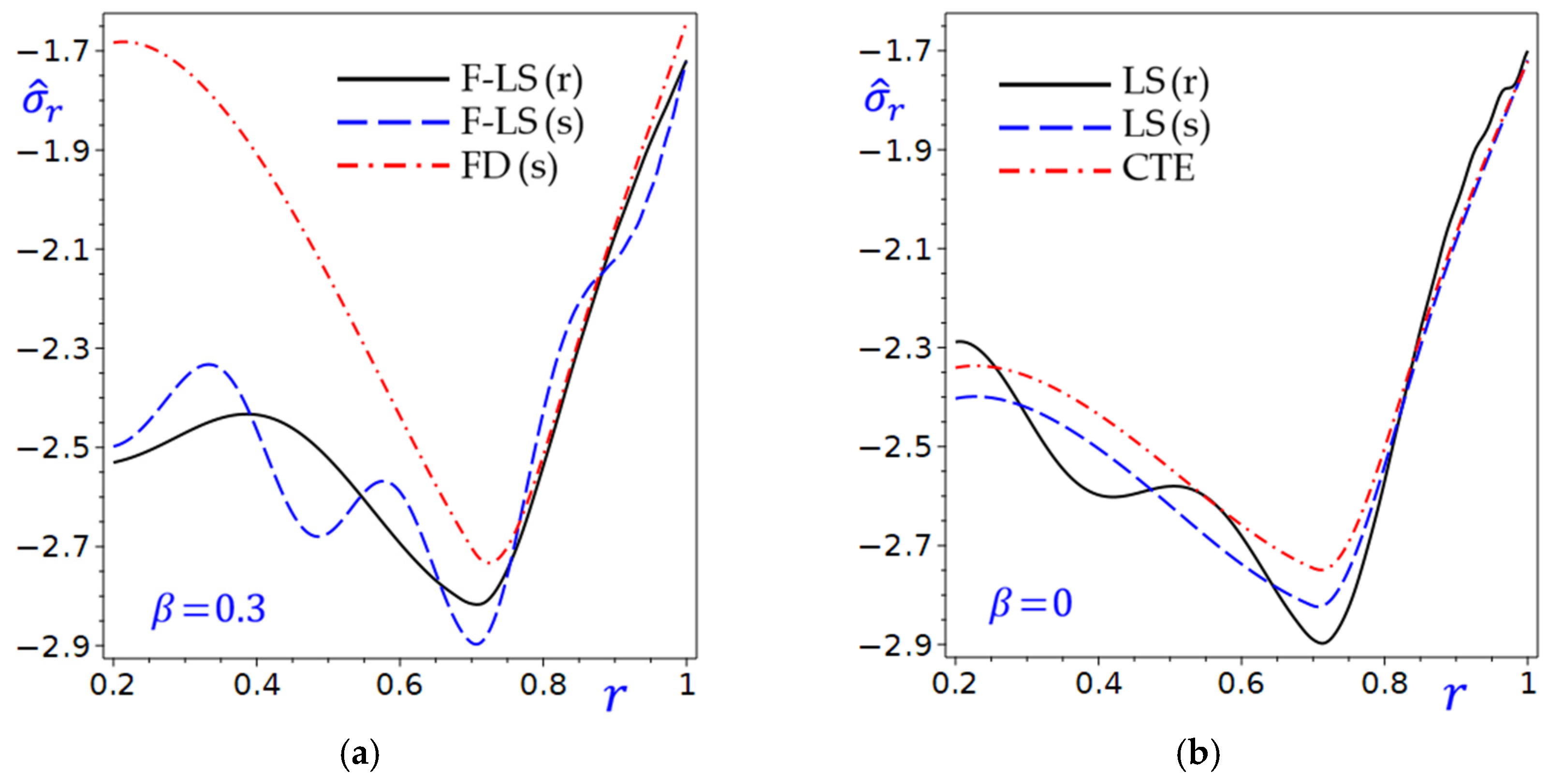
Figure 6 depicts the relationship between radial stress ${\widehat{\sigma }}_r$ of the circular cylinder and the radial direction $r$ for different theories or conditions. All theories in Figure 6a show a decreasing trend in ${\widehat{\sigma }}_r$ as $r$ increases. The curves of ${\widehat{\sigma }}_r$ may converge or diverge depending on $r$, suggesting varying performance or sensitivity of the theories under different conditions. In Figure 6b, the trend of ${\widehat{\sigma }}_r$ decreasing with $r$ persists, but the behavior of the theories may differ due to $\beta =0$. The inclusion of $r=1$ provides additional insight into the asymptotic behavior of ${\widehat{\sigma }}_r$. In fact, comparing Figure 6a,b shows how the parameter $\beta$ influences the relationship between ${\widehat{\sigma }}_r$ and $r$. The differences in trends suggest $\beta$ plays a significant role in the cylinder’s behavior.

Figure 6. The radial stress ${\widehat{\sigma }}_r$ in the circular cylinder with and without the fraction parameter: (a) $\beta =0.3$; (b) $\beta =0$.

Figure 6. The radial stress ${\widehat{\sigma }}_r$ in the circular cylinder with and without the fraction parameter: (a) $\beta =0.3$; (b) $\beta =0$.

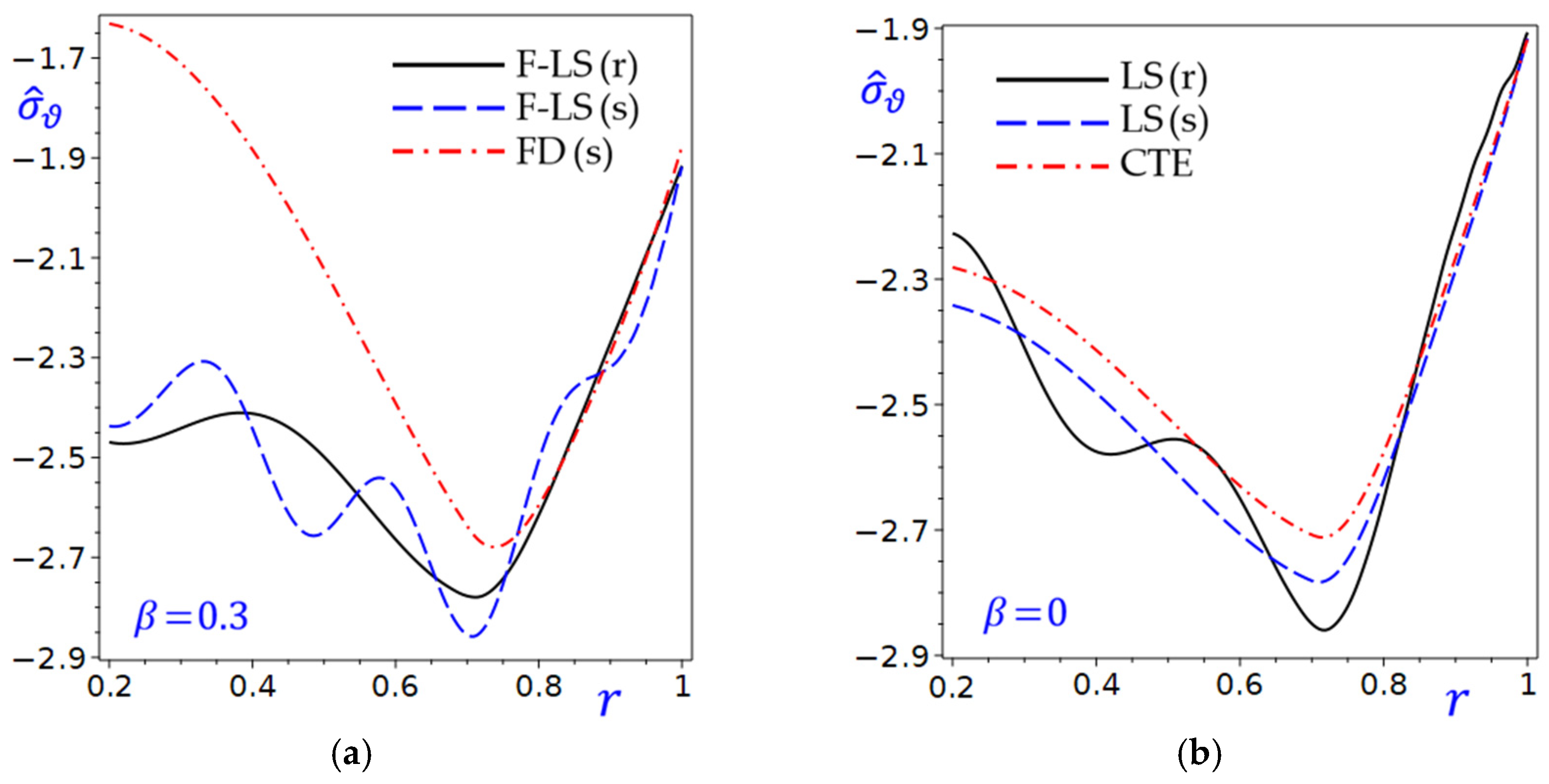
Figure 7 shows the hoop stress ${\widehat{\sigma }}_{\vartheta }$ of the circular cylinder with and without the fraction parameter (a) $\beta =0.3$ (b) $\beta =0$. The performance of all theories in Figure 7a degrades (values of ${\widehat{\sigma }}_{\vartheta }$ become more negative) as $r$ increases. The F-LS (r) and F-LS (s) theories may overlap or perform similarly, while the FD (s) theory shows a different trend, possibly worse performance of ${\widehat{\sigma }}_{\vartheta }$ at higher $r$. The refined and simple F-LS theories may outperform the FD (s) theory at higher $r$. In Figure 7b, all theories show a decline in performance (more negative values of ${\widehat{\sigma }}_{\vartheta }$) as $r$ increases. The CTE theory appears to perform ${\widehat{\sigma }}_{\vartheta }$ worse than LS (r) and LS (s) theories across most $r$ values. The LS(r) theory outperforms the CTE and LS (s) theories, with variants possibly being similar. Increasing $r$ negatively impacts performance in both plots, suggesting it may control a trade-off. The difference between plots suggests $\beta$ influences the behavior of the theories. For example, $\beta =0.3$ may lead to better performance for F-LS theories in Figure 7a compared to $\beta =0$ in Figure 7b.

Figure 7. The hoop stress ${\widehat{\sigma }}_{\vartheta }$ in the circular cylinder with and without the fraction parameter: (a) $\beta =0.3$; (b) $\beta =0$.

Figure 7. The hoop stress ${\widehat{\sigma }}_{\vartheta }$ in the circular cylinder with and without the fraction parameter: (a) $\beta =0.3$; (b) $\beta =0$.

4.2. Effect of Fractional Parameter $\beta$

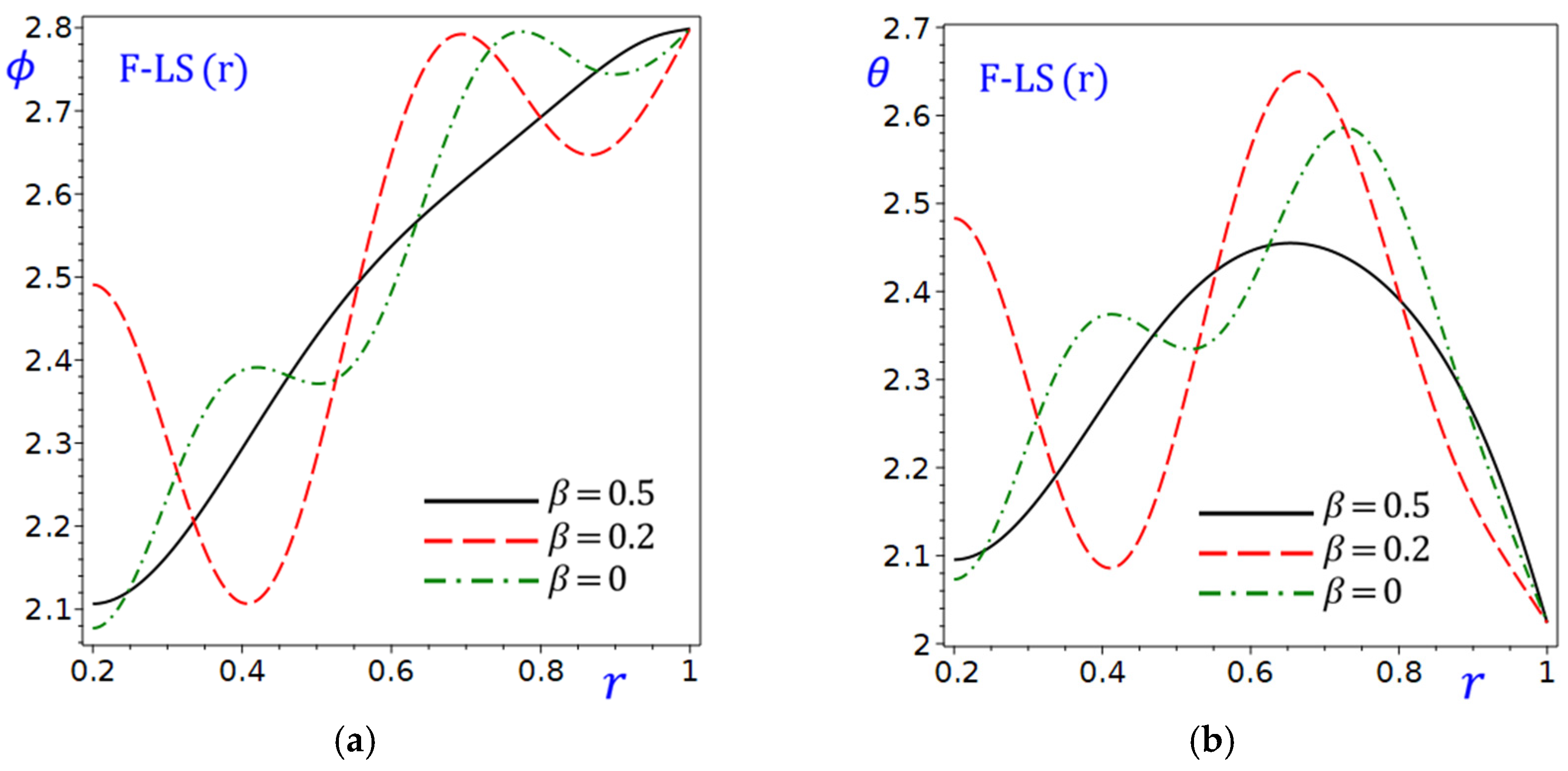
Figure 8a shows the effect of the fractional parameter $\beta$ of the circular cylinder on the temperature-mapping $\varphi$ due to the refined F-LS (r) theory.

Figure 8. Effect of fractional parameter $\beta$ of the circular cylinder due to the refined F-LS (r) theory: (a) temperature-mapping $\varphi$; (b) temperature $\theta$.

Figure 8. Effect of fractional parameter $\beta$ of the circular cylinder due to the refined F-LS (r) theory: (a) temperature-mapping $\varphi$; (b) temperature $\theta$.

The figure involves the fractional parameter $\beta$ with values 0.5, 0.2, and 0. The curve of $\varphi$ for $\beta =0.5$ is the increasing function of $r.$ The curve for $\beta =0.2$ starts at the highest value of $\varphi$ (around 2.5) and decreases sharply as $r$ increases, peaking around $r=0.4,$ then increases rapidly as $r$ increases, peaking once again around $r=0.66,$ then decreases as $r$ increases with a third peaking around $r=0.87$. The curve of $\varphi$ for $\beta =0$ may be similar to that for $\beta =0.2$. Figure 8b shows the effect of the fractional parameter $\beta$ of the circular cylinder on the temperature $\theta$ due to the refined F-LS (r) theory. The curve for $\beta =0.2$ starts at the highest value of $\theta$ (around 2.5) and decreases sharply as $r$ increases, peaking around $r=0.4,$ then increases rapidly as $r$ increases, peaking once again around $r=0.66$. The curves for $\beta =0$ and $\beta =0.5$ start at a lower value (around 2.1) and increase more gradually. In general, Figure 8 illustrates how the temperature-mapping $\varphi$ and the temperature $\theta$ vary with $r$ for different $\beta$ values due to the refined F-LS (r) theory. The figure highlights the role of $\beta$ in determining the sensitivity of $\varphi$ and $\theta$ to changes in $r$. The trends suggest that careful selection of $\beta$ is crucial for optimizing the performance or output represented by $\varphi$ and $\theta$ due to the refined F-LS (r) theory.

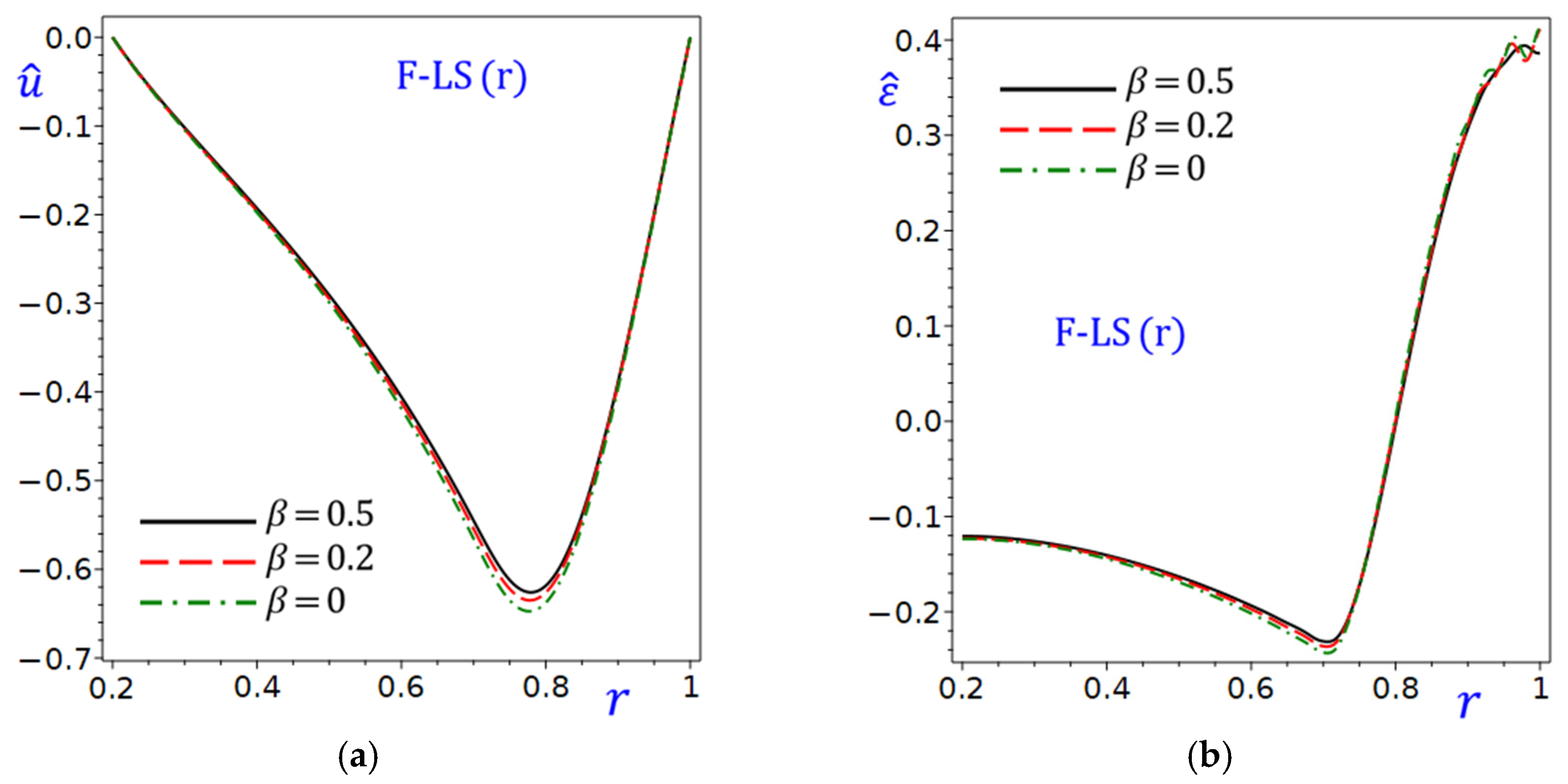
Figure 9a shows the effect of the fractional parameter $\beta$ of the circular cylinder on displacement $\widehat{u}$ due to the refined F-LS (r) theory. For all $\beta$ values (0, 0.2, 0.5), $\widehat{u}$ due to the F-LS (r) theory decreases (becomes more negative) as $r$ increases. The rate of decrease is more pronounced for higher $\beta$ values. For example, $\beta =0.5$ shows a steeper decline of $\widehat{u}$ compared to $\beta =0$. At $r=0.78$, the displacement $\widehat{u}$ reaches its lowest value, with $\beta =0$ yielding the most negative result. Figure 9b shows the effect of the fractional parameter $\beta$ of the circular cylinder on the dilatation $\widehat{\epsilon }$ due to the refined F-LS (r) theory. For $\beta =0$, $\widehat{\epsilon }$ remains relatively stable or slightly decreases as $r$ increases. For $\beta =0.2$ and $\beta =0.5$, $\widehat{\epsilon }$ decreases more significantly as $r$ increases, with $\beta =0.5$ showing the steepest decline. At $r=0.71$, $\widehat{\epsilon }$ becomes negative for all $\beta$, indicating a potential over-correction or instability in the cylinder. In general, higher $\beta$ values lead to more pronounced changes in both $\widehat{u}$ and $\widehat{\epsilon }$ as $r$ increases. This suggests that $\beta$ amplifies the sensitivity of these metrics to $r$. Increasing $r$ generally leads to a decrease in both $\widehat{u}$ and $\widehat{\epsilon }$, with the effect being more dramatic for larger $\beta$ values.

Figure 9. Effect of fractional parameter $\beta$ of the circular cylinder due to the refined F-LS (r) theory: (a) displacement $\widehat{u}$; (b) dilatation $\widehat{\epsilon }$.

Figure 9. Effect of fractional parameter $\beta$ of the circular cylinder due to the refined F-LS (r) theory: (a) displacement $\widehat{u}$; (b) dilatation $\widehat{\epsilon }$.

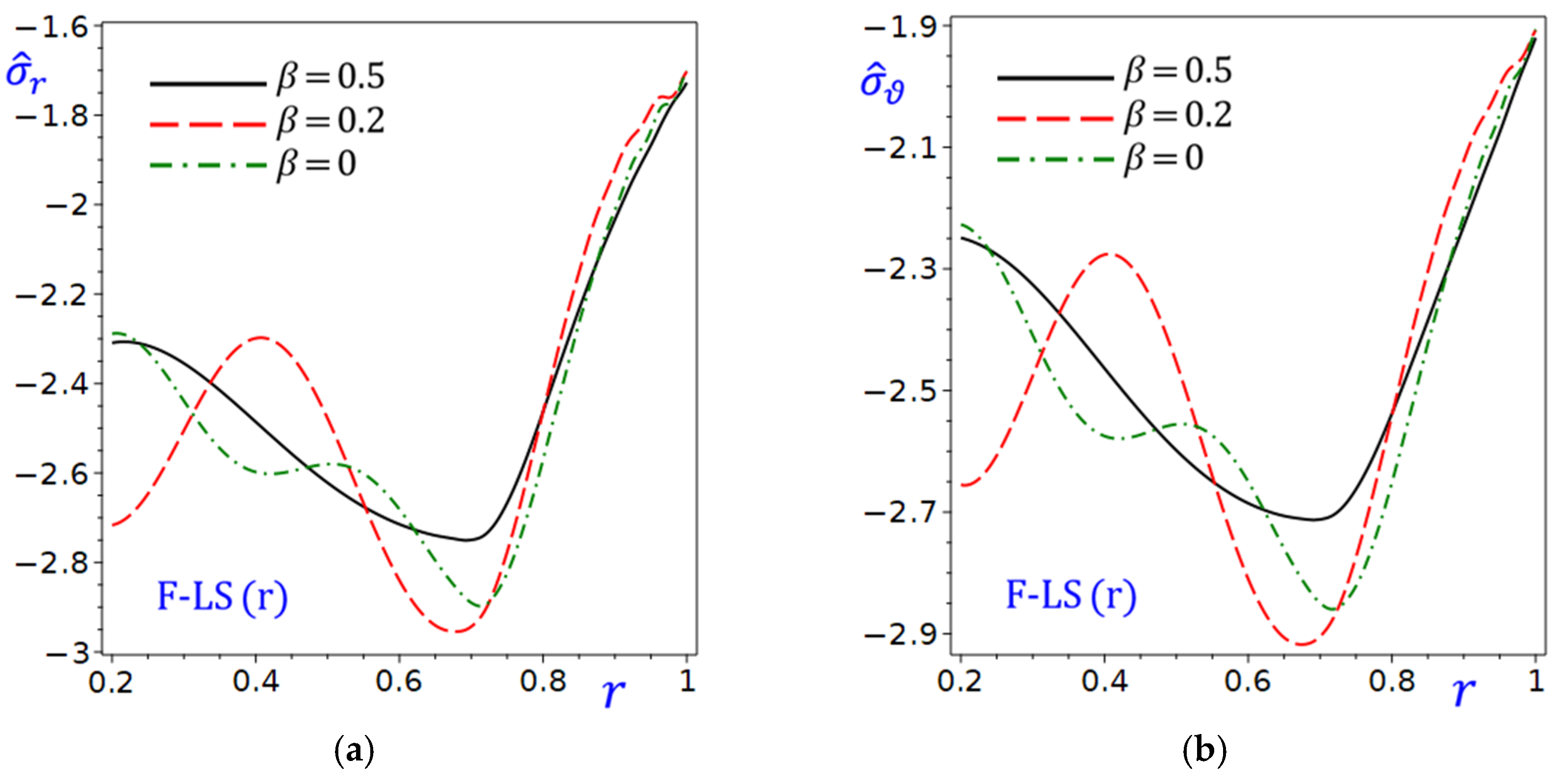
Figure 10 shows the effect of the fractional parameter $\beta$ on the radial ${\widehat{\sigma }}_r$ and hoop ${\widehat{\sigma }}_{\vartheta }$ stresses of the circular cylinder due to the refined F-LS (r) theory. The radial stress ${\widehat{\sigma }}_r$ in Figure 10a ranges is approximately $-1.6$ to $-3$. For all $\beta$ values, ${\widehat{\sigma }}_r$ becomes more negative (i.e., compressive stress increases) as $r$ increases. Higher $\beta$ values (e.g., $\beta =0.5$) result in less compressive ${\widehat{\sigma }}_r$ compared to lower $\beta$ values (e.g., $\beta =0$). The curves are smooth and monotonically decreasing, suggesting a consistent radial stress gradient. The hoop stress ${\widehat{\sigma }}_{\vartheta }$ in Figure 10b shows similar curves to Figure 10a, ${\widehat{\sigma }}_{\vartheta }$ becomes more compressive as $r$ increases. Higher $\beta$ values lead to less compressive hoop stresses, with $\beta =0.5$ showing the least compressive behavior. The curves are smooth and exhibit a consistent gradient, though the drop is steeper compared to ${\widehat{\sigma }}_r$. In general, the fractional parameter $\beta$ reduces compressive stresses in both radial and hoop directions as it increases. The trend suggests $\beta$ may correlate with stiffness or a non-dimensional load parameter. Both ${\widehat{\sigma }}_r$ and ${\widehat{\sigma }}_{\vartheta }$ are compressive (negative) across the domain, typical of confined or pressurized structures. The hoop stresses ${\widehat{\sigma }}_{\vartheta }$ are generally more compressive than radial stresses ${\widehat{\sigma }}_r$.

Figure 10. Effect of fractional parameter $\beta$ of the circular cylinder due to the refined F-LS (r) theory: (a) radial stress ${\widehat{\sigma }}_r$; (b) hoop stress ${\widehat{\sigma }}_{\vartheta }$.

Figure 10. Effect of fractional parameter $\beta$ of the circular cylinder due to the refined F-LS (r) theory: (a) radial stress ${\widehat{\sigma }}_r$; (b) hoop stress ${\widehat{\sigma }}_{\vartheta }$.

4.3. Effect of Thermal Conductivity Parameter ${\kappa }_1$

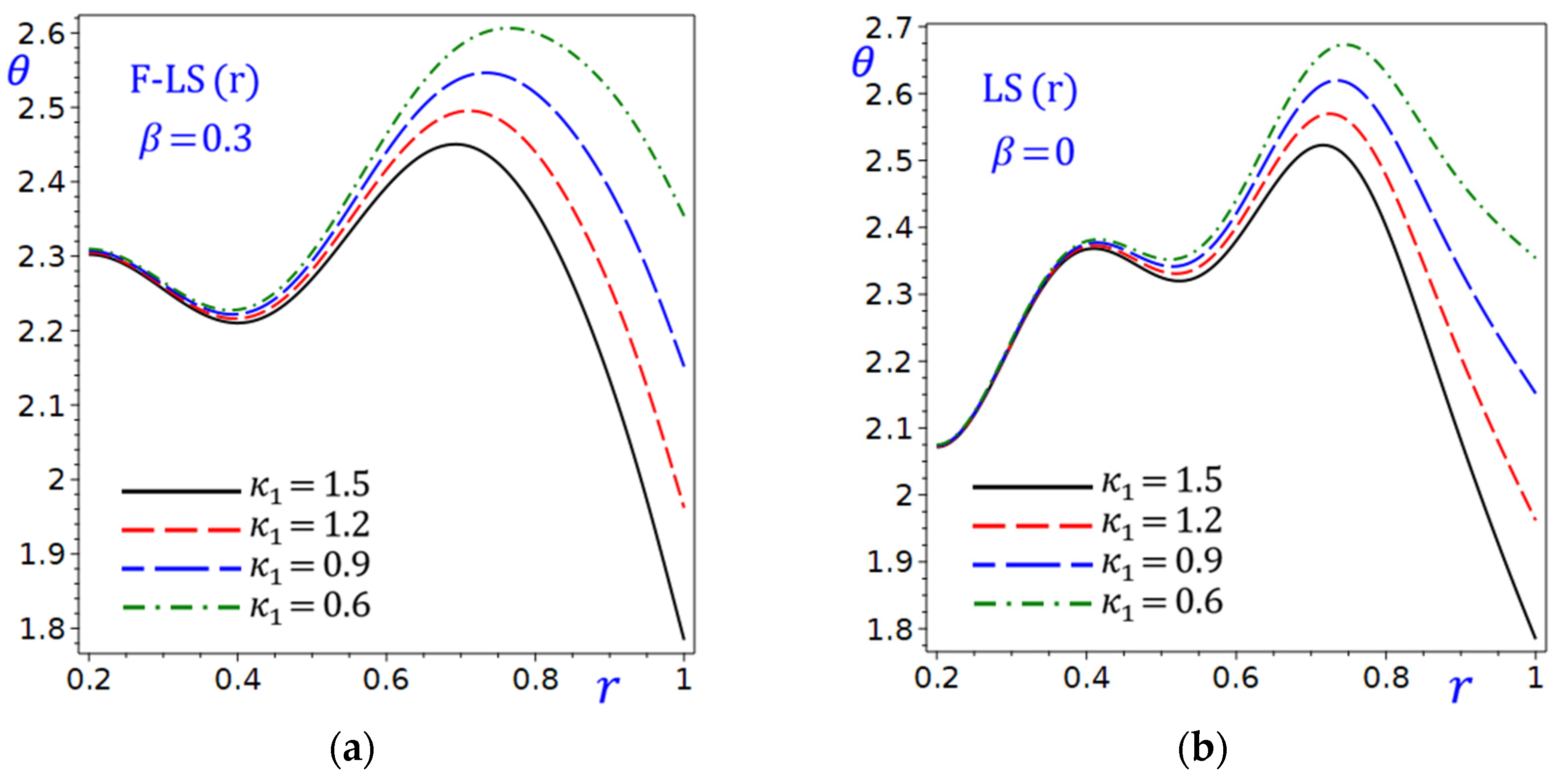
Figure 11 depicts the relationship between the temperature $\theta$ and the radial direction of the cylinder $r$ for different values of the thermal conductivity parameter ${\kappa }_1$ under two distinct conditions: F-LS (r) theory with $\beta =0.3$ in Figure 11a and LS (r) theory with $\beta =0$ in Figure 11b.

Figure 11. Effect of thermal conductivity parameter ${\kappa }_1$ on the temperature $\theta$ of the circular cylinder due to the refined: (a) F-LS (r); (b) LS (r) theories.

Figure 11. Effect of thermal conductivity parameter ${\kappa }_1$ on the temperature $\theta$ of the circular cylinder due to the refined: (a) F-LS (r); (b) LS (r) theories.

In both plots, $\theta$ decreases as $r$ increases, indicating an inverse relationship between the two variables. The rate of decrease in $\theta$ is more pronounced at lower values of $r$ and tends to stabilize as $r$ approaches 1. Higher values of the thermal conductivity parameter ${\kappa }_1$ (e.g., 1.5) result in lower $\theta$ values across all $r$, while lower values of ${\kappa }_1$ (e.g., 0.6) lead to higher $\theta$ values. This suggests that ${\kappa }_1$ non-positively influences $\theta$. The separation between curves for different ${\kappa }_1$ values is consistent, indicating that the effect of ${\kappa }_1$ on $\theta$ is uniform across the range of $r$. In Figure 11b, the temperature $\theta$ values are generally higher compared to those in Figure 11a for all values of ${\kappa }_1$ values. This implies that the presence of $\beta =0.3$ in the F-LS (r) theory increases $\theta$.

In Figure 12, the effects of the thermal conductivity parameter ${\kappa }_1$ on the radial displacement $\widehat{u}$ of the circular cylinder due to the refined F-LS (r) and LS (r) theories are presented. In Figure 12a, four curves are plotted for different values of ${\kappa }_1$: 1.5, 1.2, 0.9, and 0.6. All curves start near $r=0.2$ and decrease monotonically as $r$ increases. Higher ${\kappa }_1$ values (e.g., 1.5) result in a slower decline, while lower ${\kappa }_1$ values (e.g., 0.6) lead to a steeper drop. The negative slope of $\widehat{u}$ suggests that increasing ${\kappa }_1$ reduces the response $r$. The effect is more pronounced for smaller ${\kappa }_1$, indicating that ${\kappa }_1$ modulates the sensitivity of $r$ to $\widehat{u}$. In Figure 12b, the plot of $\widehat{u}$ due to the LS (r) theory with $\beta =0$ is considered. All curves of $\widehat{u}$ start at 0 and decrease as $r$ increases. Higher ${\kappa }_1$ values again result in a gentler decline, while lower ${\kappa }_1$ values cause a sharper drop.

Figure 12. Effect of thermal conductivity parameter ${\kappa }_1$ on the radial displacement $\widehat{u}$ of the circular cylinder due to the refined: (a) F-LS (r); (b) LS (r) theories.

Figure 12. Effect of thermal conductivity parameter ${\kappa }_1$ on the radial displacement $\widehat{u}$ of the circular cylinder due to the refined: (a) F-LS (r); (b) LS (r) theories.

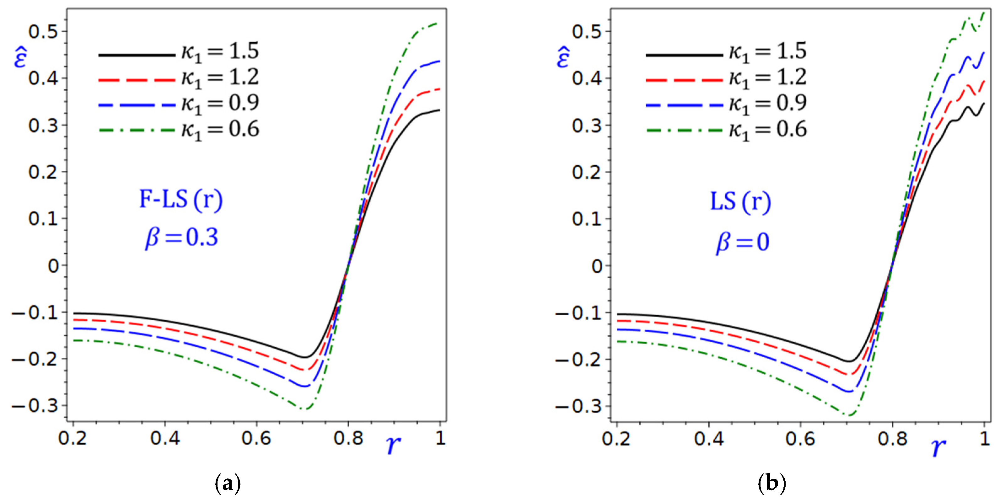
Figure 13 shows the effect of the thermal conductivity parameter ${\kappa }_1$ on the dilatation $\widehat{\epsilon }$ of the circular cylinder due to the refined F-LS (r) and LS (r) theories. Both plots show $\widehat{\epsilon }$ decreasing as $r$ increases, indicating that $0.2\le r\le 0.7$ leads to reduced dilatation. At $r=0.8$, the dilatation vanishes irrespective of the value of the thermal conductivity parameter ${\kappa }_1$. The curves for different ${\kappa }_1$ values are distinct, suggesting that ${\kappa }_1$ significantly influences the dilatation behavior. Higher ${\kappa }_1$ values (e.g., 1.5) result in higher $\widehat{\epsilon }$ values in $0.2\le r\le 0.8$ and lower $\widehat{\epsilon }$ values in $0.8<r\le 1$. This implies that ${\kappa }_1$ is not directly proportional to the dilatation measure. In Figure 13a, the curves exhibit the same pronounced decrease in $\widehat{\epsilon }$ with increasing $r$ as in Figure 13b, indicating that the presence of $\widehat{\epsilon }$ has little sensitivity to the variation of $\widehat{\epsilon }$. For $r$ close to 0, $\widehat{\epsilon }$ is at its local highest, and the difference between curves for varying ${\kappa }_1$ is most noticeable. As $r$ approaches 0.8, $\widehat{\epsilon }$ trends toward zero or a minimal value, with the curves converging. The maximum values of $\widehat{\epsilon }$ occur at the outer surface of the cylinder.

Figure 13. Effect of thermal conductivity parameter ${\kappa }_1$ on the dilatation $\widehat{\epsilon }$ of the circular cylinder due to the refined: (a) F-LS (r); (b) LS (r) theories.

Figure 13. Effect of thermal conductivity parameter ${\kappa }_1$ on the dilatation $\widehat{\epsilon }$ of the circular cylinder due to the refined: (a) F-LS (r); (b) LS (r) theories.

Figure 14 shows the effect of the thermal conductivity parameter ${\kappa }_1$ on the radial stress ${\widehat{\sigma }}_r$ of the circular cylinder due to the refined F-LS (r) and LS (r) theories. Figure 14a represents the radial stress ${\widehat{\sigma }}_r$, ranging from $-1.6$ to $-3$ in four curves, each corresponding to a different value of the thermal conductivity parameter ${\kappa }_1$ (1.5, 1.2, 0.9, 0.6). The negative values suggest compressive stress due to the fractional F-LS (r) theory with $\beta =0.3$. The trend indicates that as ${\kappa }_1$ decreases, the radial stress ${\widehat{\sigma }}_r$ becomes more negative (i.e., compressive stress increases or stress magnitude rises). Also, Figure 14b represents similar results as in Figure 14a due to the LS (r) theory $\beta =0$. The trend shows ${\widehat{\sigma }}_r$ decreasing (becoming more negative) as $r$ increases. In comparison to Figure 14a, the absence of the fractional parameter $\beta$ tends to the LS (r) theory suggesting this plot represents a simpler case (e.g., no fracture condition). In both plots, the radial stress becomes more negative as $r$ increases, indicating higher compressive stresses. Higher ${\kappa }_1$ values result in less negative ${\widehat{\sigma }}_r$, implying that ${\kappa }_1$ moderates the radial stress response. The fractional parameter $\beta$ differs between plots (0.3 in Figure 14a, 0 in Figure 14b), suggesting it influences the radial stress behavior. A non-zero $\beta$ may introduce additional nonlinearity or coupling effects.

Figure 14. Effect of thermal conductivity parameter ${\kappa }_1$ on the radial stress ${\widehat{\sigma }}_r$ of the circular cylinder due to the refined: (a) F-LS (r); (b) LS (r) theories.

Figure 14. Effect of thermal conductivity parameter ${\kappa }_1$ on the radial stress ${\widehat{\sigma }}_r$ of the circular cylinder due to the refined: (a) F-LS (r); (b) LS (r) theories.

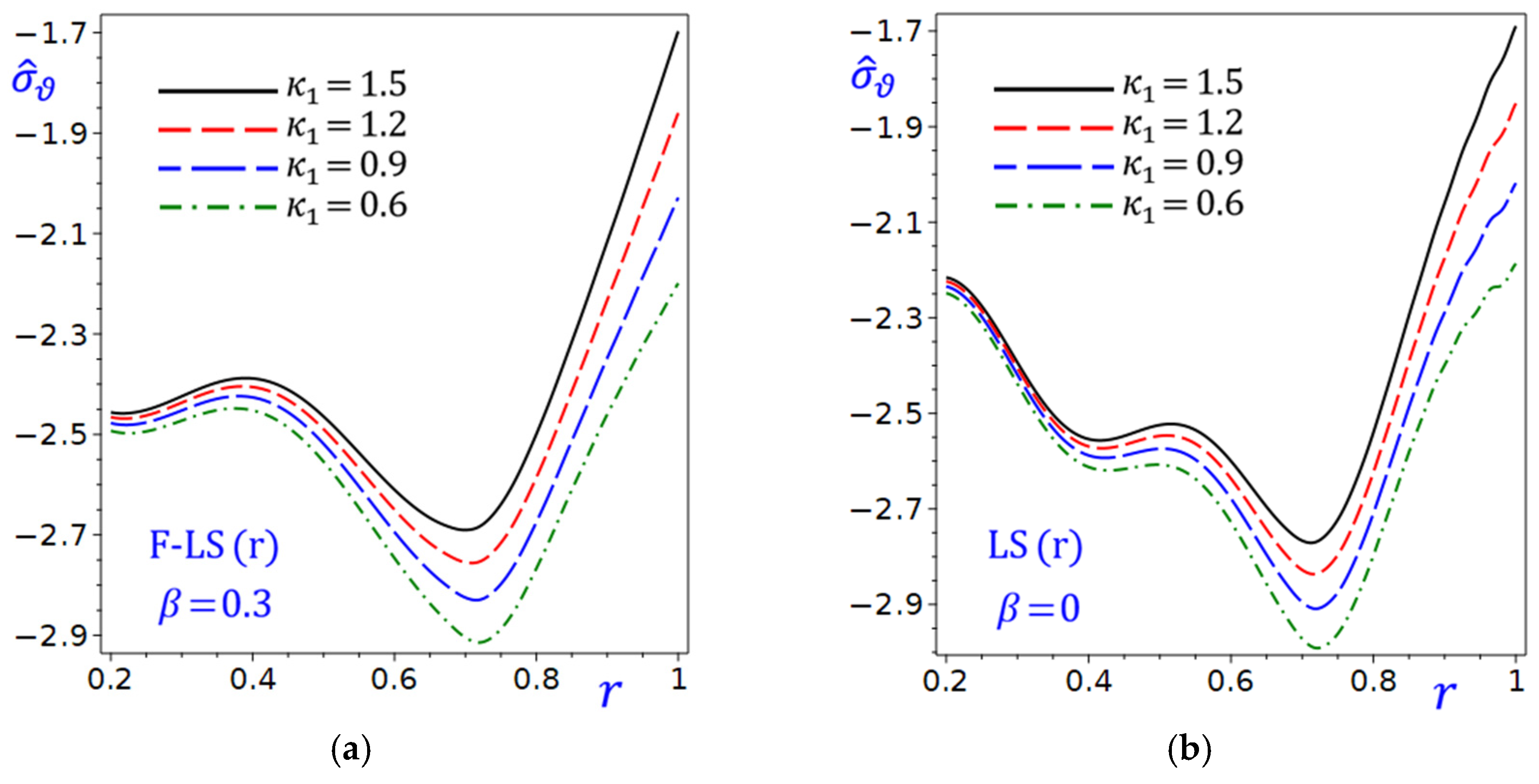
Figure 15 shows the effect of the thermal conductivity parameter ${\kappa }_1$ on the hoop stress ${\widehat{\sigma }}_{\vartheta }$ of the circular cylinder due to the refined F-LS (r) and LS (r) theories.

Figure 15. Effect of thermal conductivity parameter ${\kappa }_1$ on the hoop stress ${\widehat{\sigma }}_{\vartheta }$ of the circular cylinder due to the refined: (a) F-LS (r); (b) LS (r) theories.

Figure 15. Effect of thermal conductivity parameter ${\kappa }_1$ on the hoop stress ${\widehat{\sigma }}_{\vartheta }$ of the circular cylinder due to the refined: (a) F-LS (r); (b) LS (r) theories.

In both plots, as $r$ increases, the hoop stress ${\widehat{\sigma }}_{\vartheta }$ generally decreases (improves), but the rate of improvement varies with the thermal conductivity parameter ${\kappa }_1$. The smallest hoop stress ${\widehat{\sigma }}_{\vartheta }$ occurs around $r\approx 0.73$. Higher ${\kappa }_1$ values (e.g., 1.5) tend to perform worse (higher ${\widehat{\sigma }}_{\vartheta }$) compared to lower ${\kappa }_1$ values (e.g., 0.6) during the radial direction. The F-LS (r) theory (with $\beta =0.3$) appears to outperform LS theory ($\beta =0$) across most $r$ and ${\kappa }_1$ values, as its hoop stress ${\widehat{\sigma }}_{\vartheta }$ is consistently lower. The gap between theories is more pronounced at lower $r$ values, suggesting F-LS theory is particularly beneficial when $r$ is small. For both theories, smaller ${\kappa }_1$ values (e.g., 0.6) lead to better performance (lower ${\widehat{\sigma }}_{\vartheta }$), especially at higher $r$. The influence of ${\kappa }_1$ diminishes as $r$ increases, with all curves converging toward similar performance.

4.4. Effect of the Exponential Decay Time Parameter $t_0$

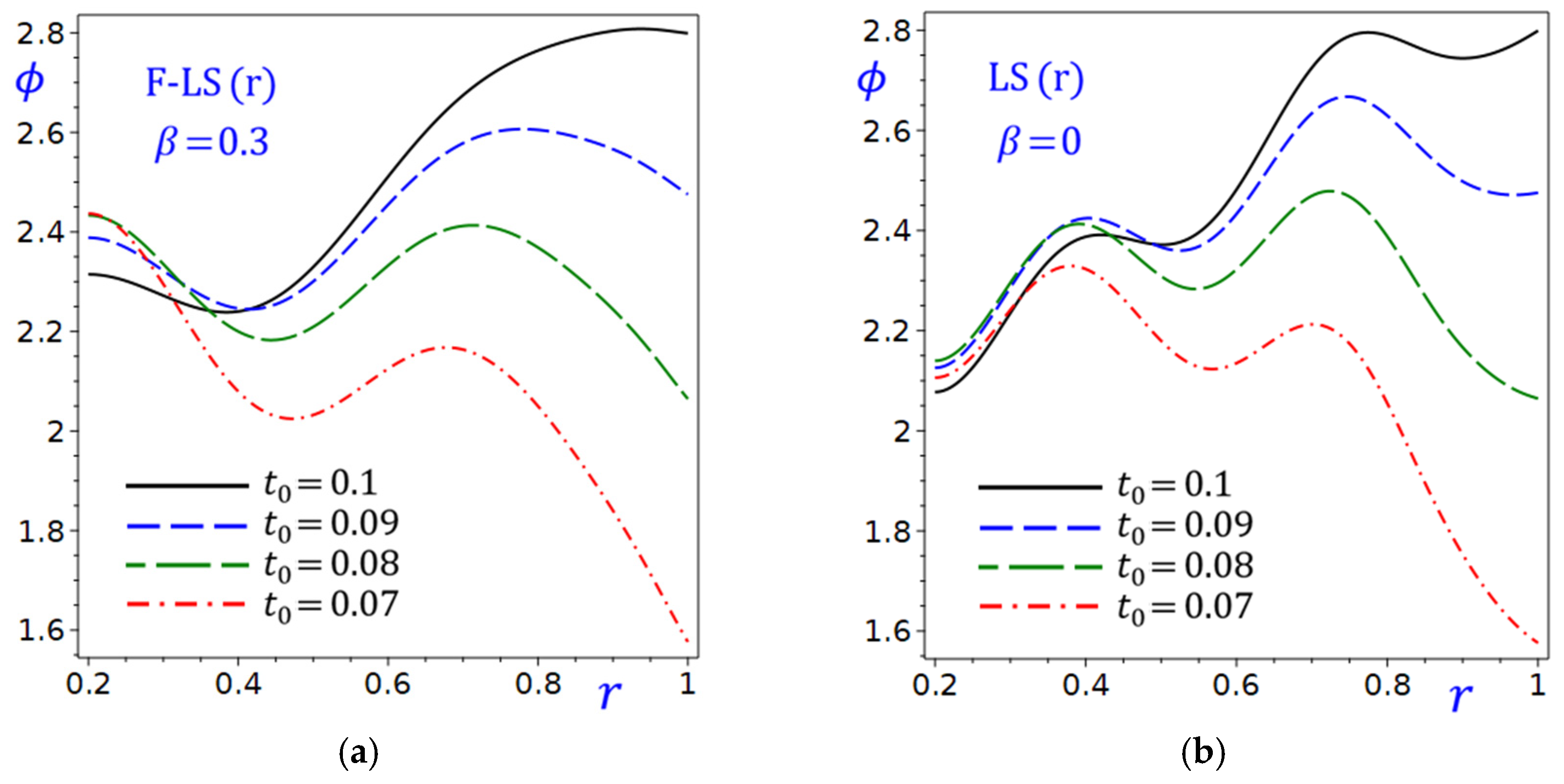
Figure 16 depicts the behavior of the temperature-mapping $\varphi$ as a function of the radial direction, under different conditions.

Figure 16. Effect of exponential decay time $t_0$ on the temperature-mapping $\varphi$ of the circular cylinder due to the refined: (a) F-LS (r); (b) LS (r) theories.

Figure 16. Effect of exponential decay time $t_0$ on the temperature-mapping $\varphi$ of the circular cylinder due to the refined: (a) F-LS (r); (b) LS (r) theories.

In Figure 16a, the fractional F-LS (r) theory with $\beta =0.3$ is used to perform $\varphi$ against $r$. Curves are plotted for different values of the exponential decay time $t_0$. It is to be noted that as $t_0$ decreases, the curves shift downward, indicating $\varphi$ decreases. The temperature-mapping $\varphi$ appears to decrease monotonically with $r$, suggesting that higher $r$ suppresses the temperature-mapping $\varphi$. The separation between curves increases as $r$ grows, showing $t_0$ has a stronger effect at larger $r$. In Figure 16b, the LS (r) theory with $\beta =0$ performs all curves, which are flatter compared to those in Figure 16a, suggesting $\varphi$ is more sensitive to $r$ and $t_0$. As $t_0$ decreases, $\varphi$ decreases uniformly across all $r$, similar to Figure 16a. The lack of curvature in Figure 16a implies $\beta =0.3$ simplifies the behavior, possibly removing nonlinear effects. In Figure 16b ($\beta =0$), $\varphi$ varies more strongly with $r$, while in Figure 16a ($\beta =0.3$), $\varphi$ is almost linear in $r$. The effect of $t_0$ is consistent in both plots: smaller $t_0$ reduces $\varphi$.

Figure 17 shows the effect of the exponential decay time $t_0$ on the temperature $\theta$ of the circular cylinder due to the refined F-LS (r) and LS (r) theories. In both plots, the temperature $\theta$ is decreasing as $r$ increases, indicating an inverse relationship. The temperature curves are monotonically decreasing, suggesting that higher values of $r$ correspond to lower values of $\theta$. In Figure 17a, the fractional F-LS (r) theory with $\beta =0.3$ is used to perform multiple curves for different values of the exponential decay time $t_0$ (0.1, 0.09, 0.08, 0.07), showing how $\theta$ varies with $r$ for each $t_0$. As $t_0$ decreases, the $\theta$ values shift downward, indicating that smaller $t_0$ results in lower $\theta$ for the same $r$. In Figure 17b the LS (r) theory with $\beta =0$ performs curves similar to Figure 17a for the same $t_0$ values. The trend is analogous to Figure 17a, but the temperature $\theta$ values are generally higher for the same $r$ and $t_0$. This suggests that $\beta =0.3$ in Figure 17a may lead to lower $\theta$ values than $\beta =0$ in Figure 17b.

Figure 17. Effect of exponential decay time $t_0$ on the temperature $\theta$ of the circular cylinder due to the refined: (a) F-LS (r); (b) LS (r) theories.

Figure 17. Effect of exponential decay time $t_0$ on the temperature $\theta$ of the circular cylinder due to the refined: (a) F-LS (r); (b) LS (r) theories.

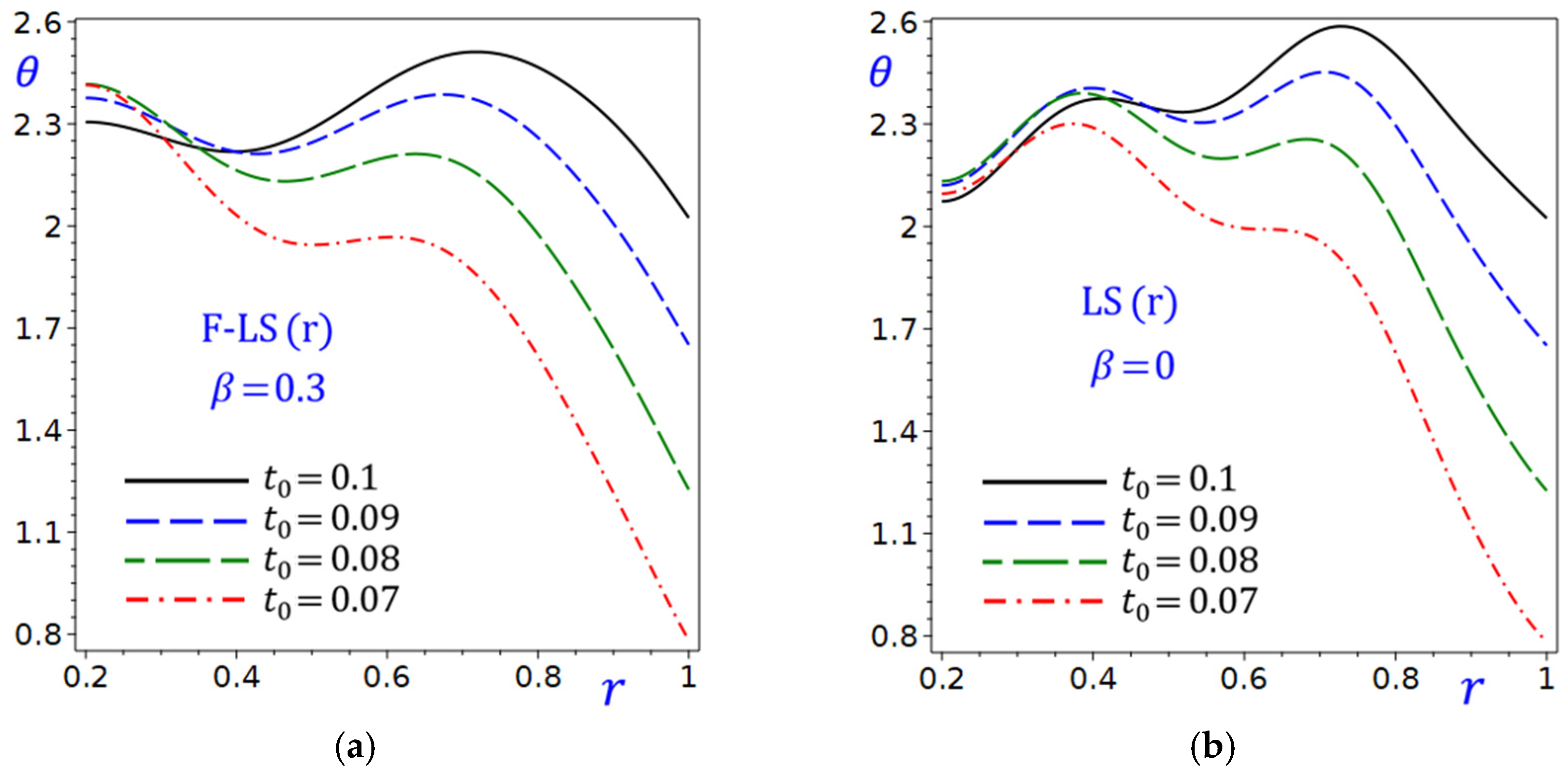
The effect of the exponential decay time $t_0$ on the radial displacement $\widehat{u}$ of the circular cylinder due to the refined F-LS (r) and LS (r) theories is presented in Figure 18. The curves of the radial displacement $\widehat{u}$ in Figure 18a, show how the displacement varies with $r$ for different values of the exponential decay time $t_0$. All curves of $\widehat{u}$ start near 0 and decrease monotonically as $r$ increases. The smallest value of $\widehat{u}$ occurs at $r=0.76$. Smaller values of the exponential decay time $t_0$ (e.g., 0.07) result in slightly worse performance (more negative values) compared to larger $t_0$ (e.g., 0.1). In Figure 18b, similar plots to those in Figure 18a but with $\beta =0$, indicating a different configuration. The curves exhibit a steeper decline compared to Figure 18a, suggesting that $\beta =0$ leads to more sensitivity to $r$. The impact of $t_0$ is less pronounced here, with all curves closely clustered.

Figure 18. Effect of exponential decay time $t_0$ on the radial displacement $\widehat{u}$ of the circular cylinder due to the refined: (a) F-LS (r); (b) LS (r) theories.

Figure 18. Effect of exponential decay time $t_0$ on the radial displacement $\widehat{u}$ of the circular cylinder due to the refined: (a) F-LS (r); (b) LS (r) theories.

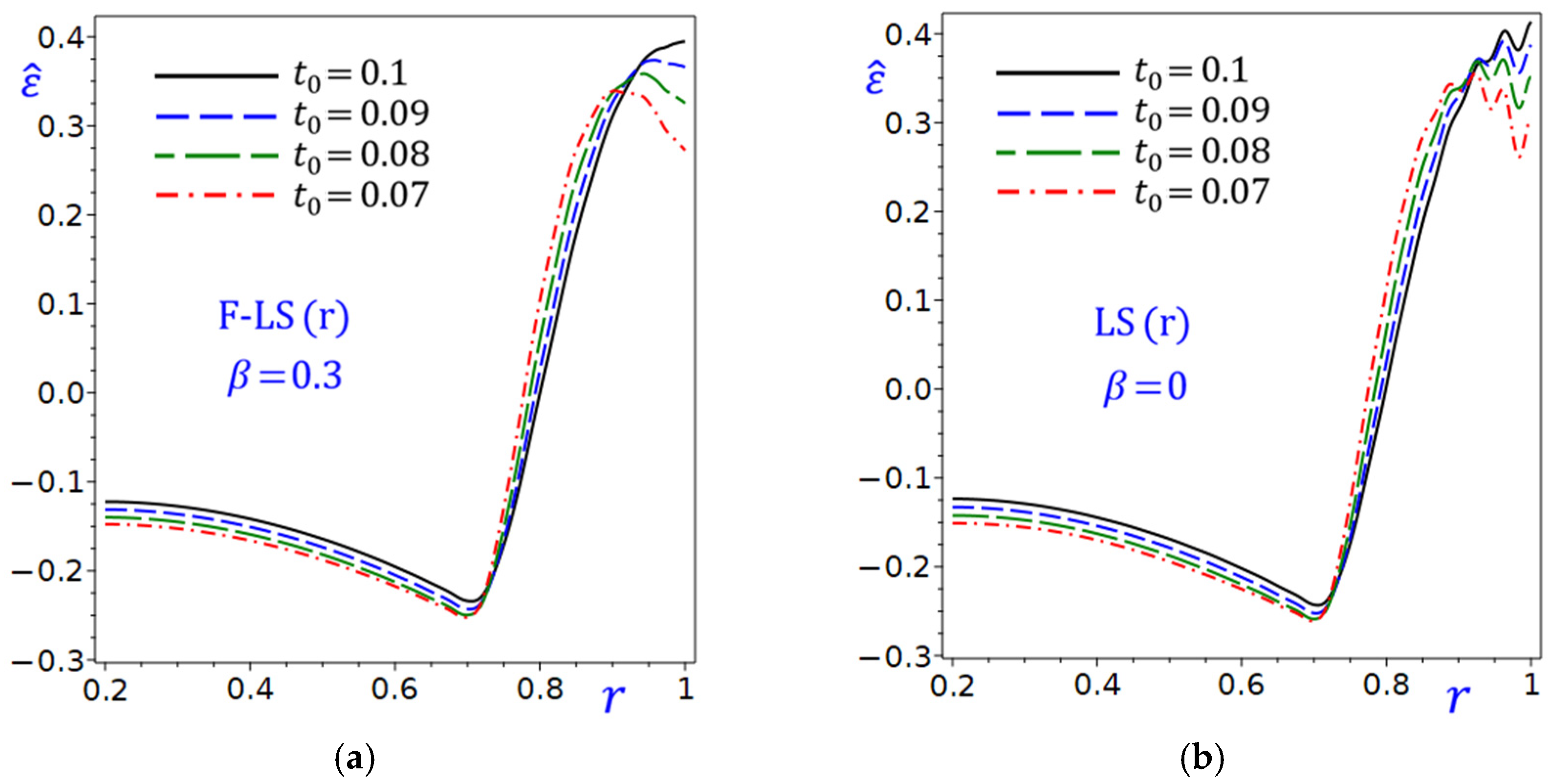
Figure 19 depicts the behavior of the dilatation $\widehat{\epsilon }$ as a function of $r$. Both plots represent the dilatation $\widehat{\epsilon }$, ranging from $-0.3$ to $0.4$, versus the radial direction of the circular cylinder due to the refined F-LS (r) and LS (r) theories. Four curves are shown in Figure 19a due to F-LS (r) theory with $\beta =0.3$, each corresponding to a different value of $t_0$: 0.1, 0.09, 0.08, and 0.07. The dilatation $\widehat{\epsilon }$ exhibits variability concerning $r$, with peaks and troughs indicating sensitivity to the radial direction. The curves for different $t_0$ values are distinct, suggesting that $t_0$ significantly influences the behavior of dilatation $\widehat{\epsilon }$. The dilatation $\widehat{\epsilon }$ in Figure 19b shows a different trend compared to that in Figure 19a, with smoother variations across $r$ due to the LS (r) theory with $\beta =0$. The curves for different $t_0$ values are closely spaced, indicating that $t_0$ has the same pronounced effect on $\widehat{\epsilon }$ as in Figure 19b. The fractional component in F-LS introduces additional complexity, as seen in the more pronounced variability of $\widehat{\epsilon }$. The dilatation $\widehat{\epsilon }$ due to the LS theory is more sensitive to changes in $t_0$ especially for higher $r$.

Figure 19. Effect of exponential decay time $t_0$ on the dilatation $\widehat{\epsilon }$ of the circular cylinder due to the refined: (a) F-LS (r); (b) LS (r) theories.

Figure 19. Effect of exponential decay time $t_0$ on the dilatation $\widehat{\epsilon }$ of the circular cylinder due to the refined: (a) F-LS (r); (b) LS (r) theories.

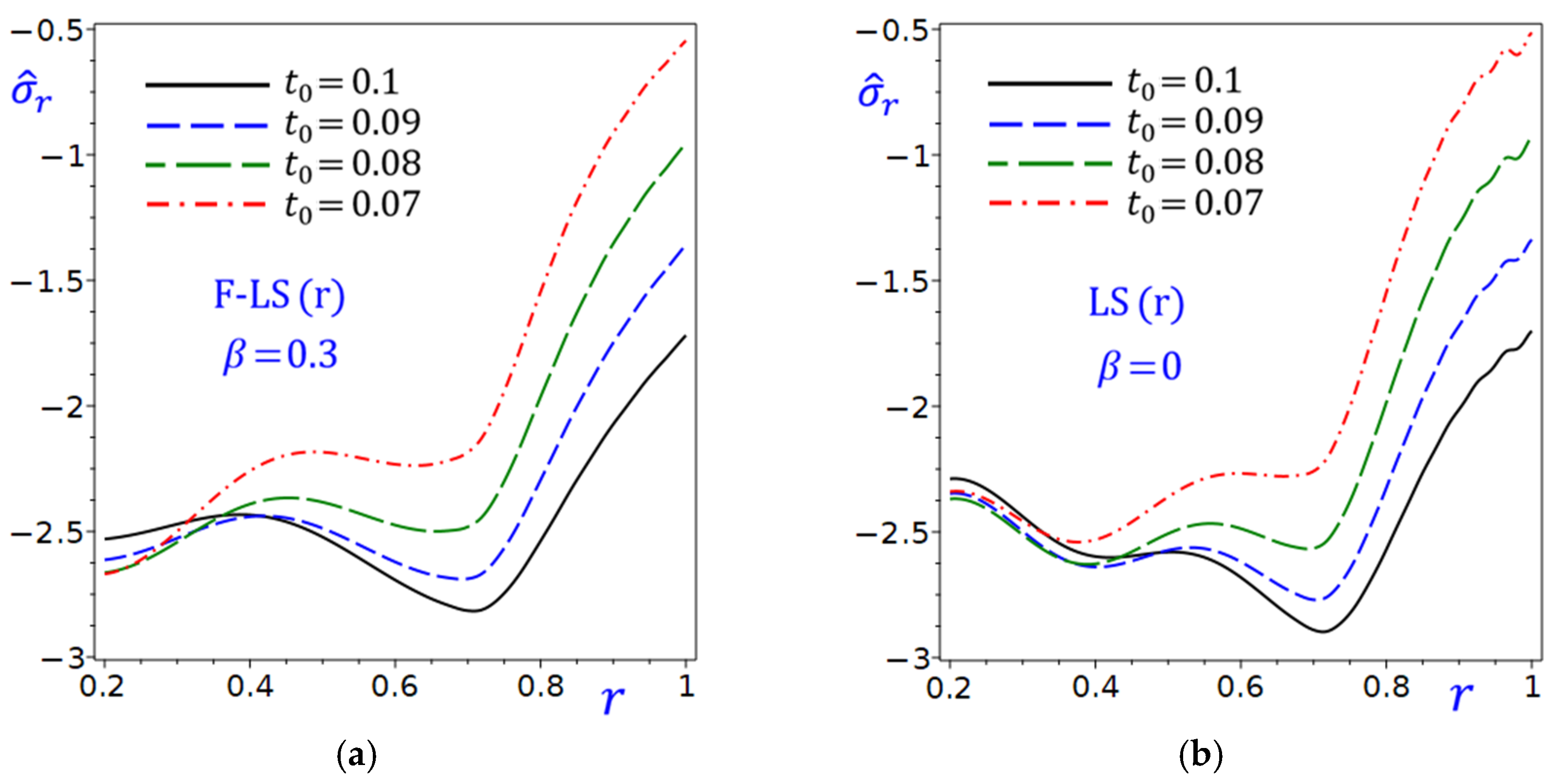
The provided plots in Figure 20 depict the behavior of the radial stress component ${\widehat{\sigma }}_r$ as a function of the radial coordinate $r$ for different exponential decay time $t_0$ and fractional parameter $\beta$. The plots in Figure 20a represent the radial stress ${\widehat{\sigma }}_r$ which vary radially, indicated by the F-LS (r) theory with $\beta =0.3$. The radial stress ${\widehat{\sigma }}_r$ starts below $-2.5$ and increases monotonically toward $-0.5$ as $r$ approaches 1. The curves for different $t_0$ values (0.1, 0.09, 0.08, 0.07) overlap closely, suggesting that the exponential decay time $t_0$ has a minimal effect on the radial stress distribution for this $\beta$ value. The radial stress is compressive across the entire domain but diminishes toward the outer edge ($r=1$). The insensitivity to $t_0$ implies that the stress distribution is dominated by the fractional parameter $\beta$ rather than geometric factors in this regime. The compressive nature of ${\widehat{\sigma }}_r$ could indicate residual stress or external pressure loading. The plots in Figure 20b represent ${\widehat{\sigma }}_r$ under similar conditions due to the LS (r) theory with $\beta =0$. The radial stress ${\widehat{\sigma }}_r$ starts below $-2$ and increases monotonically toward $-0.5$ as $r$ approaches 1, showing a nonlinear drop. The curves for different $t_0$ values are distinct, indicating that the exponential decay time $t_0$ significantly influences stress distribution. Stress becomes more compressive toward the outer edge, like in Figure 20a.

Figure 20. Effect of exponential decay time $t_0$ on the radial stress ${\widehat{\sigma }}_r$ in the circular cylinder due to the refined: (a) F-LS (r); (b) LS (r) theories.

Figure 20. Effect of exponential decay time $t_0$ on the radial stress ${\widehat{\sigma }}_r$ in the circular cylinder due to the refined: (a) F-LS (r); (b) LS (r) theories.

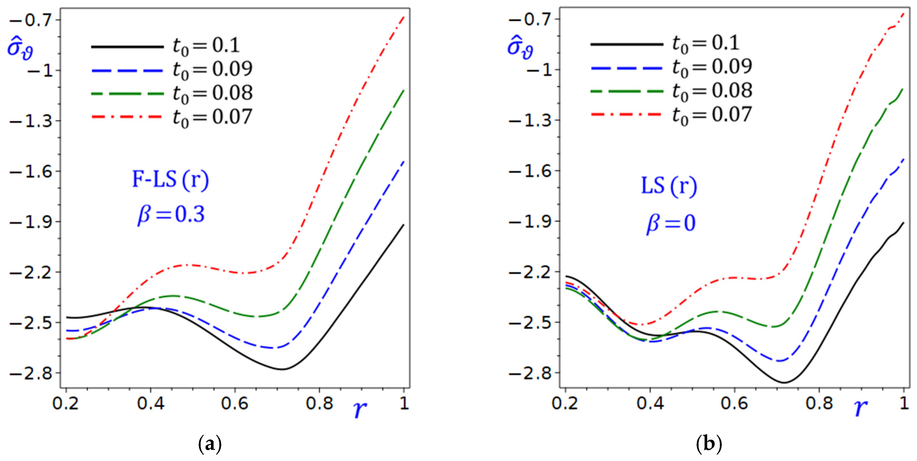
Figure 21 shows the effect of the exponential decay time $t_0$ on the hoop stress ${\widehat{\sigma }}_{\vartheta }$ of the circular cylinder due to the refined F-LS (r) and LS (r) theories. In Figure 21a, the hoop stress ${\widehat{\sigma }}_{\vartheta }$ due to the F-LS (r) theory is plotted along the radial direction of the cylinder. As $t_0$ decreases (from 0.1 to 0.07), the hoop stress ${\widehat{\sigma }}_{\vartheta }$ becomes more negative, indicating higher volatility or dispersion. The relationship between $r$ and ${\widehat{\sigma }}_{\vartheta }$ is not explicitly shown, but the trend suggests that smaller $t_0$ leads to larger deviations. Similarly to Figure 21a, decreasing $t_0$ results in more negative ${\widehat{\sigma }}_{\vartheta }$ values as shown in Figure 21b. The trend concerning $r$ is unclear, but the lines may diverge as $r$ increases.

Figure 21. Effect of exponential decay time $t_0$ on the hoop stress ${\widehat{\sigma }}_{\vartheta }$ in the circular cylinder due to the refined: (a) F-LS (r); (b) LS (r) theories.

Figure 21. Effect of exponential decay time $t_0$ on the hoop stress ${\widehat{\sigma }}_{\vartheta }$ in the circular cylinder due to the refined: (a) F-LS (r); (b) LS (r) theories.

5. Conclusions

This study developed a fractional thermoelastic model to analyze the thermal response of a circular cylinder with variable thermal conductivity, formulated within the framework of the generalized Lord–Shulman theory incorporating fractional derivatives. The Laplace transform was employed to convert the time-dependent governing equations into ordinary differential equations, and the resulting solutions were numerically inverted to the time domain. Graphical representations were provided to illustrate the variations in field variables along the radial direction of the cylinder.

The results reveal that the fractional parameter $\beta$ plays a significant role in controlling the thermal and mechanical responses. An increase in $\beta$ leads to higher temperature distributions, indicating that the fractional effect influences the thermal baseline. The radial stress ${\widehat{\sigma }}_r$ decreases with increasing radial distance $r$, confirming an inverse relationship between stress and radius. Furthermore, the fractional model (F-LS) demonstrates enhanced sensitivity compared to the standard LS theory, suggesting that it provides a more refined characterization of the thermoelastic response.

The analysis also shows that the radial displacement $\widehat{u}$ and dilatation $\widehat{\epsilon }$ exhibit strong dependence on both r and $\beta$. Larger $\beta$ values, especially at higher $r$, induce substantial changes in $\widehat{\epsilon }$, implying that careful parameter selection is necessary to maintain mechanical stability. The observed negative $\widehat{\epsilon }$ values at large $r$ and $\beta$ warrant further investigation to ensure the reliability of the model in such regimes.

Additionally, spatial variations in the radial ${\widehat{\sigma }}_r$ and hoop ${\widehat{\sigma }}_{\vartheta }$ stresses indicate that higher $\beta$ values mitigate compressive stresses, potentially improving the load-bearing capacity and reducing failure risks in structural applications. The thermal conductivity parameter ${\kappa }_1$ is also identified as a key factor affecting temperature evolution, with the fractional formulation (F-LS) showing higher sensitivity to ${\kappa }_1$ than the classical LS model.

The exponential decay time $t_0$ significantly influences the temperature, displacement, and stress behavior. Smaller $t_0$ values lead to sharper gradients and higher stress magnitudes, whereas larger $t_0$ values result in smoother distributions. The fractional LS model effectively moderates these variations, demonstrating its capability to damp extreme stress responses.

Overall, the fractional Lord–Shulman formulation provides an improved and more flexible representation of coupled thermoelastic phenomena in materials with variable thermal conductivity. The interplay among $\beta$, ${\kappa }_1$, and $t_0$ offers valuable insights for the design and optimization of advanced thermoelastic systems, enabling better control of thermal and mechanical performance under complex loading conditions.

References

1. Zenkour, A.M.; Abouelregal, A.E. Nonlocal thermoelastic vibrations for variable thermal conductivity nanobeams due to harmonically varying heat. J. Vibroeng. 2014, 16, 3665–3678. [Google Scholar]
2. Othman, M.I.A.; Abouelregal, A.E. Magnetothermoelstic analysis for an infinite solid cylinder with variable thermal conductivity due to harmonically varying heat. Microsyst. Technol. 2017, 23, 5635–5644. [Google Scholar] [CrossRef]
3. Xiong, C.-B.; Yu, L.-N.; Niu, Y.-B. Effect of variable thermal conductivity on the generalized thermoelasticity problems in a fiber-reinforced anisotropic half-space. Adv. Mater. Sci. Eng. 2019, 2019, 8625371. [Google Scholar] [CrossRef]
4. Lotfy, K. Effect of variable thermal conductivity during the photothermal diffusion process of semiconductor medium. Silicon 2019, 11, 1863–1873. [Google Scholar] [CrossRef]
5. Abbas, I.; Hobiny, A.; Marin, M. Photo-thermal interactions in a semi-conductor material with cylindrical cavities and variable thermal conductivity. J. Taibah Univ. Sci. 2020, 14, 1369–1376. [Google Scholar] [CrossRef]
6. Bajpai, A.; Sharma, P.K.; Kumar, R. Transient response of a thermo-diffusive elastic thick circular plate with variable conductivity and diffusivity. Acta Mech. 2021, 232, 3343–3361. [Google Scholar] [CrossRef]
7. Bajpai, A.; Sharma, P.K. Variable thermal conductivity and diffusivity impact on forced vibrations of thermodiffusive elastic plate. J. Therm. Stresses 2021, 44, 1169–1190. [Google Scholar] [CrossRef]
8. Mahdy, A.M.S.; Lotfy, K.; Hassan, W.; El-Bary, A.A. Analytical solution of magneto-photothermal theory during variable thermal conductivity of a semiconductor material due to pulse heat flux and volumetric heat source. Waves Random Complex Media 2021, 31, 2040–2057. [Google Scholar] [CrossRef]
9. Alhejaili, W.; Lotfy, K.; El-Bary, A. Thermodiffusion waves of mechanical ramp non-local excited semiconductor medium with variable thermal conductivity. Silicon 2022, 14, 12707–12719. [Google Scholar] [CrossRef]
10. Hobiny, A.; Abbas, I. Generalized thermoelastic interaction in orthotropic media under variable thermal conductivity using the finite element method. Mathematics 2023, 11, 955. [Google Scholar] [CrossRef]
11. Said, S.M. A study on the frame of a memory-dependent derivative in a micropolar thermoelastic medium under the effect of the variable thermal conductivity. Mech. Adv. Mater. Struct. 2023, 51, 665–681. [Google Scholar] [CrossRef]
12. Mahdy, A.M.S.; Lotfy, K.; El-Bary, A.; Roshdy, E.M.; Abd El-Raouf, M.M. Variable thermal conductivity during photo-thermoelasticy theory of semiconductor medium induced by laser pulses with hyperbolic two-temperature theory. Waves Random Complex Media 2024, 34, 2877–2899. [Google Scholar] [CrossRef]
13. Tiwari, R.; Sachan, S.; Abouelregal, A.; Kumar, R.; Elzayady, M.E. Viscothermoelastic vibrations on circular microplate resonators using the Moore–Gibson–Thompson thermal-conductivity model. Mech. Time-Depend. Mater. 2024, 28, 1291–1311. [Google Scholar] [CrossRef]
14. Hamza, F.; Abdou, M.; Abd El-Latief, A.M. Generalized fractional thermoelasticity associated with two relaxation times. J. Therm. Stresses 2014, 37, 1080–1098. [Google Scholar] [CrossRef]
15. Hussein, E.M. Fractional order thermoelastic problem for an infinitely long solid circular cylinder. J. Therm. Stresses 2015, 38, 133–145. [Google Scholar] [CrossRef]
16. Hussein, E.M. One-dimensional problem for infinitely long annular cylinder in the context of fractional order theory of thermoelasticity. Z. Angew. Math. Mech. 2016, 96, 1482–1489. [Google Scholar] [CrossRef]
17. Hamza, F.; Abd El-Latief, A.M.; Abdou, M. 1D applications on fractional generalized thermoelasticity associated with two relaxation times. Mech. Adv. Mater. Struct. 2016, 23, 689–703. [Google Scholar] [CrossRef]
18. Abbas, I.A. Fractional order generalized thermoelasticity in an unbounded medium with cylindrical cavity. J. Eng. Mech. 2016, 142, 04016033-1. [Google Scholar] [CrossRef]
19. Ezzat, M.A.; El-Karamany, A.S.; El-Bary, A.A. Application of fractional order theory of thermoelasticity to 3D time-dependent thermal shock problem for a half-space. Mech. Adv. Mater. Struct. 2017, 24, 27–35. [Google Scholar] [CrossRef]
20. Molla, M.A.K.; Mondal, N.; Mallik, S.H. Effects of fractional and two-temperature parameters on stress distributions for an unbounded generalized thermoelastic medium with spherical cavity. Arab. J. Basic Appl. Sci. 2019, 26, 302–310. [Google Scholar] [CrossRef]
21. Kumar, N.; Kamdi, D.B. Thermal behavior of a finite hollow cylinder in context of fractional thermoelasticity with convection boundary conditions. J. Therm. Stresses 2020, 43, 1189–1204. [Google Scholar] [CrossRef]
22. Abouelregal, A.E. Modified fractional thermoelasticity model with multi-relaxation times of higher order: Application to spherical cavity exposed to a harmonic varying heat. Waves Random Complex Media 2021, 31, 812–832. [Google Scholar] [CrossRef]
23. Tiwari, R.; Abouelregal, A.E. Thermo-viscoelastic transversely isotropic rotating hollow cylinder based on three-phase lag thermoelastic model and fractional Kelvin–Voigt type. Acta Mech. 2022, 233, 2453–2470. [Google Scholar] [CrossRef]
24. Sherief, H.H.; Hussein, E.M. Fractional order model of micropolar thermoelasticity and 2D half-space problem. Acta Mech. 2023, 234, 535–552. [Google Scholar] [CrossRef]
25. Geetanjali, G.; Sharma, P.K. Impact of fractional strain on medium containing spherical cavity in the framework of generalized thermoviscoelastic diffusion. J. Therm. Stresses 2023, 46, 333–350. [Google Scholar] [CrossRef]
26. Youssef, H.M. Fractional-order strain of an infinite annular cylinder based on Caputo and Caputo–Fabrizio fractional derivatives under hyperbolic two-temperature generalized thermoelasticity theory. J. Umm Al-Qura Univ. Eng. Archit. 2024, 15, 431–445. [Google Scholar] [CrossRef]
27. Geetanjali, G.; Sharma, P.K. Vibrational analysis of transversely isotropic hollow cylinder based on fractional generalized thermoelastic diffusion models with nonlocal effects. Acta Mech. 2024, 235, 147–166. [Google Scholar] [CrossRef]
28. Sherief, H.H.; Hussein, E.M. New fractional order model of thermoporoelastic theory for a porous infinitely long cylinder saturated with fluid. Waves Random Complex Media 2024, 34, 4754–4783. [Google Scholar] [CrossRef]
29. Al-Lehaibi, E.A.N.; Youssef, H.M. The influence of the Caputo fractional derivative on time-fractional Maxwell’s equations of an electromagnetic infinite body with a cylindrical cavity under four different thermoelastic theorems. Mathematics 2024, 12, 3358. [Google Scholar] [CrossRef]
30. Youssef, H.M. Mathematical modeling of time-fractional Maxwell’s equations on a magnetothermoelastic half-space under Green–Naghdi theorems and of Caputo definition. Mathematics 2025, 13, 1094. [Google Scholar] [CrossRef]
31. Povstenko, Y.Z. Fractional cattaneo-type equations and generalized thermoelasticity. J. Therm. Stresses 2011, 34, 97–114. [Google Scholar] [CrossRef]
32. Abo-Dahab, S.M.; Abbas, I.A. LS model on thermal shock problem of generalized magneto-thermoelasticity for an infinitely long annular cylinder with variable thermal conductivity. Appl. Math. Model. 2011, 35, 3759–3768. [Google Scholar] [CrossRef]
33. Pal, P.; Kar, A.; Kanoria, M. Fractional order generalised thermoelasticity to an infinite body with a cylindrical cavity and variable material properties. Eur. J. Comput. Mech. 2014, 23, 96–111. [Google Scholar] [CrossRef]
34. Sherief, H.; Hamza, F. Modeling of variable thermal conductivity in a generalized thermoelastic infinitely long hollow cylinder. Meccanica 2016, 51, 551–558. [Google Scholar] [CrossRef]
35. Ezzat, M.; El-Bary, A. On thermo-viscoelastic infinitely long hollow cylinder with variable thermal conductivity. Microsyst. Technol. 2017, 23, 3263–3270. [Google Scholar] [CrossRef]
36. Zenkour, A.M. Generalized thermoelasticity theories for axisymmetric hollow cylinders under thermal shock with variable thermal conductivity. J. Mol. Eng. Mater. 2018, 6, 1850006. [Google Scholar] [CrossRef]
37. Gilhotra, G.; Sharma, P.K. Visco-thermodiffusive elastic interactions in plate within the framework of two-temperature fractional thermoelastic models. Indian J. Phys. 2022, 96, 3867–3879. [Google Scholar] [CrossRef]
38. Alshaikh, F. Effects of thermal relaxation times and porosity in a Lord-Shulman and refined multi-phase lags model of generalized thermoelasticity. Mech. Based Des. Struct. Mach. 2023, 51, 438–449. [Google Scholar] [CrossRef]
39. Zenkour, A.M.; Saeed, T.; Al-Raezah, A.A. Fractional order of refined Lord–Shulman model for a 1D thermoelastic response of skin tissue due to ramp-type heating. Arch. Appl. Mech. 2024, 94, 989–1003. [Google Scholar] [CrossRef]
40. Geetanjali, G.; Sharma, P.K. Transient responses of two temperature, fractional thermo-diffusive-elastic half space with temperature dependent properties. Int. J. Comput. Methods Eng. Sci. Mech. 2024, 25, 80–96. [Google Scholar] [CrossRef]
41. Shariyat, M. Propagation and interference of oppositely traveling generalized multi-fractional-order thermo-viscoelastic waves in discs with fractional-order constitutive and heat conduction models. Waves Random Complex Media 2025, 35, 3932–3960. [Google Scholar] [CrossRef]
42. Al-Lehaibi, E.A.N. Applying Caputo and Caputo–Fabrizio fractional derivatives on a viscothermoelastic circular microplate under Lord–Shulman theorem. AIP Adv. 2025, 15, 045223. [Google Scholar] [CrossRef]
43. Zenkour, A.M.; Saeed, T.; Almalki, A.A. Thermoelastic plane strain solutions to rotating cylinders due to a refined fractional-order theory. J. Comput. Appl. Mech. 2026, 57, 11–26. [Google Scholar]
44. Lord, H.W.; Shulman, Y.A. A generalized dynamical theory of thermoelasticity. J. Mech. Phys. Solids 1967, 15, 299–309. [Google Scholar] [CrossRef]
45. Biot, M. Thermoelasticity and irreversible thermo-dynamics. J. Appl. Phys. 1956, 27, 240–253. [Google Scholar] [CrossRef]
46. Honig, G.; Hirdes, U. A method for the numerical inversion of Laplace transforms. J. Comput. Appl. Math. 1984, 10, 113–132. [Google Scholar] [CrossRef]
47. Tzou, D.Y. Experimental support for the lagging behavior in heat propagation. J. Thermophys. Heat Transf. 1995, 9, 686–693. [Google Scholar] [CrossRef]
Figure 1. Schematic and geometry of the hollow cylinder.
Mathematics 13 03497 g001
Disclaimer/Publisher’s Note: The statements, opinions and data contained in all publications are solely those of the individual author(s) and contributor(s) and not of MDPI and/or the editor(s). MDPI and/or the editor(s) disclaim responsibility for any injury to people or property resulting from any ideas, methods, instructions or products referred to in the content.