A Lambert-Type Lindley Distribution as an Alternative for Skewed Unimodal Positive Data

Abstract

This paper introduces the Lambert-Lindley distribution, a two-parameter extension of the Lindley model constructed through the Lambert-F generator. The new distribution retains the non-negative support of the Lindley distribution and provides additional flexibility by incorporating a shape parameter that controls skewness and tail behavior. Structural properties are derived, including the probability density function, cumulative distribution function, quantile function, hazard rate, and moments. Parameter estimation is addressed using the method of moments and maximum likelihood, and a Monte Carlo simulation study carried out to evaluate the performance of the proposed estimators. The practical applicability of the Lambert–Lindley distribution is demonstrated with two real datasets: stress rupture times of Kevlar/epoxy composites and hospital stay durations of breast cancer patients. Comparative analyses using goodness-of-fit tests and information criteria demonstrate that the proposed model can outperform classical alternatives such as the Gamma and Weibull distributions. Consequently, the Lambert–Lindley distribution emerges as a flexible alternative for modeling positive unimodal data in contexts such as material reliability studies and clinical duration analysis.

1. Introduction

Univariate probability distributions with positive support are fundamental in reliability engineering, biomedicine, economics, and environmental sciences. Many variables of interest, such as waiting times, lifetimes of materials, hospital stays, or environmental measurements, are non-negative by nature; see, for instance, [1,2,3,4].

In this context, the Lindley (L) distribution [5] emerged as an alternative to the exponential model, providing an improved fit for duration data characterized by an increasing hazard rate.

A random variable X is said to follow the L distribution with shape parameter $\theta >0$, denoted by $X\sim \mathrm{L}\left(\theta \right)$, if its probability density function (PDF), cumulative distribution function (CDF), and quantile function (QF) are given by

$$\begin{array}{ccc}\hfill f(x;\theta )& =& {\displaystyle \frac{{\theta }^2}{\theta +1}}(1+x)e^{-\theta x},x>0,\hfill \end{array}$$

(1)

$$\begin{array}{ccc}\hfill F(x;\theta )& =& 1-\left(1+{\displaystyle \frac{\theta x}{\theta +1}}\right)e^{-\theta x}\mathrm{and}\hfill \end{array}$$

(2)

$$\begin{array}{ccc}\hfill F^{-1}(u;\theta )& =& -1-{\displaystyle \frac{1}{\theta }}-{\displaystyle \frac{1}{\theta }}{W}_{-1}\left[(\theta +1)(u-1)e^{-(\theta +1)}\right],0<u<1,\hfill \end{array}$$

(3)

respectively, where $W_{-1}(·)$ denotes the secondary branch of the Lambert W function.

For background on the Lambert W function, see [6]; for the derivation of Equation (3), [7]; and for a review of the L distribution, [8].

Although the L distribution has been successfully applied in lifetime analysis due to its analytical simplicity and decreasing hazard rate, it exhibits limited flexibility in controlling skewness and tail behavior. In particular, its range of skewness and kurtosis values is narrower than that of the Gamma [9] and Weibull [9,10] distributions, restricting its ability to capture data with heavier tails or different degrees of asymmetry.

To overcome these limitations, several two-parameter extensions of the L distribution have been proposed in the literature, such as the generalized Lindley distribution [11], the power-Lindley distribution [12], the Marshall–Olkin–Lindley distribution [13], and the transmuted Lindley distribution [14]. These distributions, due to their higher parameter dimension, extend the flexibility of the classical L model in terms of skewness and kurtosis.

A widely used strategy for extending classical models is the application of distributional generators. This strategy has led to several well-known distributional families, including the Marshall–Olkin distributions [15], the Beta–G distributions [16], the Gamma–G distributions [17], the transmuted distributions [18], the Kumaraswamy–G distributions [19], and the alpha–power distributions [20]. These families represent flexible extensions of classical models that, by introducing additional parameters, enhance their ability to accommodate a wide range of density shapes, skewness, kurtosis, and hazard rate behaviors, reinforcing the methodological relevance of transformation-based generators in modern statistical modeling.

A more recent example within this research line is the Lambert-F generator, introduced by [21], which allows the induction of an additional shape parameter into an arbitrary baseline distribution, thus providing flexibility in terms of skewness and tail behavior. Given a baseline distribution with CDF $F(x;\eta )$, the Lambert-F generator defines a new family through the transformation

$$\begin{array}{c}\hfill G(x;\eta ,\alpha )=1-[1-F(x;\eta )]{\alpha }^{F(x;\eta )},\alpha \in (0,e),\end{array}$$

(4)

where the parameter $\alpha$ controls skewness and tail behavior. This approach has been successfully combined with classical models, producing flexible distributions capable of modeling positive data with a wide range of shapes; see, for example, [22,23,24,25,26].

The PDF and the QF associated with Equation (4) are given by

$$\begin{array}{c}\hfill g(x;\eta ,\alpha )=f(x;\eta ){\alpha }^{F(x;\eta )}\left\{1-log\left(\alpha \right)\left[1-F(x;\eta )\right]\right\}\mathrm{and}\end{array}$$

(5)

$$\begin{array}{c}\hfill Q(u;\eta ,\alpha )=\left\{\begin{array}{cc}{F}^{-1}\left[{\displaystyle \frac{1}{log\left(\alpha \right)}}{W}_0\left({\displaystyle \frac{log\left(\alpha \right)(u-1)}{\alpha }}\right)+1;\eta \right],\hfill & \mathrm{if}\alpha \ne 1,\hfill \\ F^{-1}(u;\eta ),\hfill & \mathrm{if}\alpha =1,\hfill \end{array}\right.\end{array}$$

(6)

where $f(x;\eta )$ is the PDF of the baseline distribution, $F^{-1}(·;\eta )$ denotes the associated QF, and $W_0(·)$ represents the principal branch of the Lambert W function.

In this paper, we introduce a new extension of the L distribution obtained through the Lambert-F generator, with the L distribution taken as the baseline model. The increasing demand for handling diverse types of information, including positive data, underscores the importance of having alternative probabilistic models available for data analysis, since a richer set of models enhances the chances of adequately capturing the characteristics observed in real datasets. To the best of our knowledge, a Lambert-type version of the L distribution has not yet been explored in the literature. This naturally raises the question of whether such a model can outperform well-known two-parameter distributions such as Weibull and Gamma, as well as existing extensions of the L distribution, in terms of goodness-of-fit in real-world applications.

The rest of the paper is organized as follows. In Section 2, we introduce the new extension of the L distribution and derive some of its structural properties. Section 3 discusses parameter estimation methods and presents a Monte Carlo simulation study. In Section 4, the applicability of the proposed distribution is illustrated through two real datasets. Finally, Section 5 provides concluding remarks.

The computational implementation of the distribution in the R programming language, as well as the numerical results obtained in this study, are made publicly available at https://github.com/Dcas45/Lambert-Lindley-Distribution- (accessed on 29 September 2025).

2. Lambert–Lindley Distribution

This section introduces the new extension of the L distribution.

2.1. Lambert–Lindley Random Variable

Proposition 1.

Let $F(x;\theta )$ be the CDF of the L distribution, given in Equation (1). Then, the Lambert version of the L distribution has CDF

$$\begin{array}{ccc}\hfill G(x;\theta ,\alpha )& =& 1-{\displaystyle \frac{\theta +1+\theta x}{\theta +1}}{e}^{-\theta x}{\alpha }^{1-\left({\displaystyle \frac{\theta +1+\theta x}{\theta +1}}{e}^{-\theta x}\right)},\hfill \end{array}$$

(7)

and its PDF and QF are given by

$$\begin{array}{ccc}\hfill g(x;\theta ,\alpha )& =& {\displaystyle \frac{{\theta }^2}{\theta +1}}(1+x)e^{-\theta x}{\alpha }^{1-\left({\displaystyle \frac{\theta +1+\theta x}{\theta +1}}{e}^{-\theta x}\right)}\left[1-log\left(\alpha \right){\displaystyle \frac{\theta +1+\theta x}{\theta +1}}{e}^{-\theta x}\right],\hfill \end{array}$$

(8)

$$\begin{array}{ccc}\hfill G^{-1}(u;\theta ,\alpha )& =& \left\{\begin{array}{c}c\left({\displaystyle \frac{1}{log\left(\alpha \right)}{W}_0\left[\frac{log\left(\alpha \right)(u-1)}{\alpha }\right]+1,\theta }\right),\mathrm{if}\alpha \ne 1,\hfill \\ {\displaystyle c(u,\theta ),\mathrm{if}\alpha =1,}\hfill \end{array}\right.\hfill \end{array}$$

(9)

respectively, where $x>0$, $u\in (0,1)$, $\theta >0$, $\alpha \in (0,e)$, $W_0(·)$ and $W_{-1}(·)$ denote the principal and secondary branches of the Lambert W function, and

$$\begin{array}{c}\hfill c(z,\theta )=-{\displaystyle \frac{W_{-1}\left((\theta +1)(z-1)e^{-(1+\theta )}\right)+1+\theta }{\theta }}, \mathit{for}z\in (0,1).\end{array}$$

Proof. 

As a direct consequence of the Lambert-F generator with the L baseline distribution, this result follows directly from substituting Equations (1)–(3) into (4)–(6).    □

The use of $W_0(·)$ and $W_{-1}(·)$ in Equation (9) arises naturally from the QFs of the L and Lambert-F distributions (see [7,21]). These branches ensure that the LL QF yields positive output values, thereby guaranteeing that it is well defined for all admissible parameter values.

Definition 1.

A random variable X is said to follow a Lambert–Lindley (LL) distribution with shape parameters $\theta >0$ and $\alpha \in (0,e)$, denoted by $X\sim \mathrm{LL}(\theta ,\alpha )$, if its CDF, PDF, and QF are given by Equations (7), (8) and (9), respectively.

Remark 1.

The following observations can be made regarding the PDF of the LL distribution:

(a) If $\alpha =1$, Equation (8) reduces to

$$\begin{array}{c}\hfill g(x;\theta ,\alpha =1)={\displaystyle \frac{{\theta }^2}{\theta +1}}(1+x)e^{-\theta x},x>0,\theta >0,\alpha \in (0,e),\end{array}$$

which corresponds to the PDF of the L distribution.

It is worth noting that the LL PDF is continuous and differentiable with respect to α across its domain. In particular, as $\alpha \to 1$, both the PDF and CDF of the LL distribution converge smoothly to those of the classical L distribution, ensuring model stability and continuity across parameter transitions.

(b) Considering the limiting behavior of the PDF with respect to α, we note that $g(x;\theta ,\alpha )\to 0$ for all $x>0$ as $\alpha \to 0$, indicating a degenerate case in which the probability density vanishes across the support. Conversely, when $\alpha \to e$, the PDF converges to

$$\begin{array}{c}\hfill \underset{\alpha \to e}{lim}g(x;\theta ,\alpha )={\displaystyle \frac{{\theta }^2}{\theta +1}}(1+x)e^{-\theta x\left(1-{\displaystyle \frac{1}{\theta +1}}{e}^{-\theta x}\right)\left(1-e^{-\theta x}\right)}\left[1-{\displaystyle \frac{\theta +1+\theta x}{\theta +1}}{e}^{-\theta x}\right],\end{array}$$

which represents a one-parameter Lambert version of the L distribution. This limiting case yields a unimodal distribution with lower dispersion, reduced skewness, and smaller kurtosis than the classical L distribution.

(c) By analyzing the behavior of the PDF of the LL distribution at the boundaries of the support, we obtain

$$\underset{x\to 0}{lim}g(x;\theta ,\alpha )=[1-log\left(\alpha \right)]\underset{x\to 0}{lim}f(x;\theta )=[1-log\left(\alpha \right)]{\displaystyle \frac{{\theta }^2}{\theta +1}},$$

$$\underset{x\to \infty }{lim}g(x;\theta ,\alpha )=\underset{x\to \infty }{lim}f(x;\theta )=0,$$

where $f(x;\theta )$ denotes the PDF of the L distribution.

This implies that the L and LL distributions share the same density behavior at the upper bound of the support. However, at the lower bound, the LL distribution can exhibit either higher or lower density values than those of the L distribution, depending on the value of α.

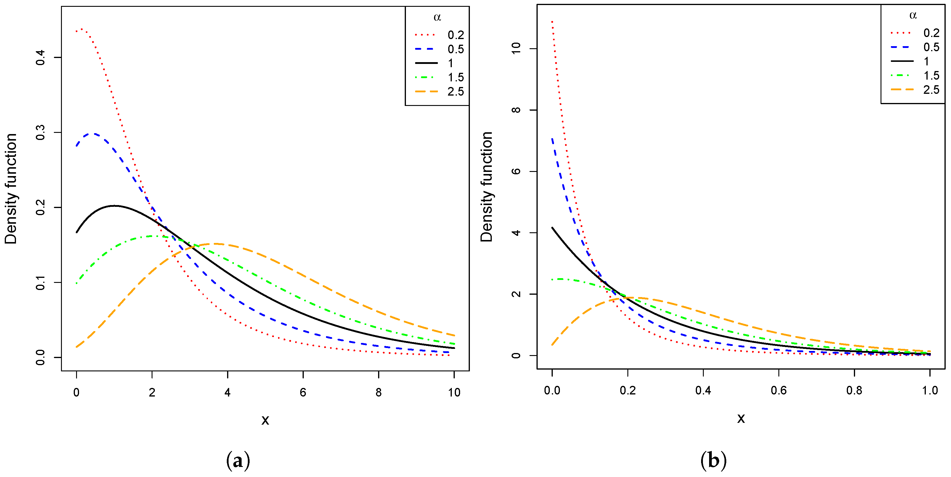
Figure 1 displays some curves of the PDF of the LL distribution for different values of the parameters $\theta$ and $\alpha$. In particular, it can be observed that the PDF may exhibit both decreasing and unimodal shapes, highlighting the flexibility of the model to represent different behaviors of positive data.

2.2. Identifiability

Proposition 2.

For the LL distribution

$$\begin{array}{c}\hfill g(x;\theta ,\alpha )=f_L(x;\theta ){\alpha }^{F_L(x;\theta )}\left\{1-log\left(\alpha \right)[1-F_L(x;\theta )]\right\},x>0,\theta >0,\alpha \in (0,e),\end{array}$$

where $f_L(·;\theta )$ and $F_L(·;\theta )$ denote the PDF and CDF of the L distribution, respectively, the parameter vector $(\theta ,\alpha )$ is identifiable; that is,

$$\begin{array}{c}\hfill g(·;{\theta }_1,{\alpha }_1)=g(·;{\theta }_2,{\alpha }_2)a.e.\mathit{on}(0,\infty )\Rightarrow ({\theta }_1,{\alpha }_1)=({\theta }_2,{\alpha }_2).\end{array}$$

Proof. 

Assume that $g(x;{\theta }_1,{\alpha }_1)=g(x;{\theta }_2,{\alpha }_2)$ for all $x>0$. As $x\to \infty$, $F_L(x;\theta )\to 1$ and

$$\begin{array}{c}\hfill g(x;\theta ,\alpha )=f_L(x;\theta ){\alpha }^{F_L(x;\theta )}\left\{1-log\left(\alpha \right)[1-F_L(x;\theta )]\right\}\sim \alpha f_L(x;\theta ).\end{array}$$

The baseline PDF $f_L(x;\theta )={\displaystyle \frac{{\theta }^2}{\theta +1}}(1+x)e^{-\theta x}$ has exponential decay governed by $\theta$. If ${\theta }_1\ne {\theta }_2$, the corresponding exponential tails differ and the equality $g(x;{\theta }_1,{\alpha }_1)=g(x;{\theta }_2,{\alpha }_2)$ cannot hold for all x, hence ${\theta }_1={\theta }_2$.

Fixing ${\theta }_1={\theta }_2=\theta$ and dividing by $f_L(x;\theta )$, we obtain

$$\begin{array}{c}\hfill {\displaystyle \frac{g(x;\theta ,\alpha )}{f_L(x;\theta )}}={\alpha }^{F_L(x;\theta )}\left[1-log\left(\alpha \right)[1-F_L(x;\theta )]\right].\end{array}$$

Taking the limit as $x\to \infty$, we have

$$\begin{array}{c}\hfill \underset{x\to \infty }{lim}{\displaystyle \frac{g(x;\theta ,{\alpha }_i)}{f_L(x;\theta )}}={\alpha }_i,i=1, 2.\end{array}$$

Since $g(·;\theta ,{\alpha }_1)\equiv g(·;\theta ,{\alpha }_2)$, these limits must coincide, implying ${\alpha }_1={\alpha }_2$. Therefore, $({\theta }_1,{\alpha }_1)=({\theta }_2,{\alpha }_2)$, and the parameters are identifiable.    □

The proof of Proposition 2 exploits the tail behavior of the LL density function, which inherits the exponential decay of the Lindley baseline. This property ensures that the parameters $\theta$ and $\alpha$ produce distinguishable effects on the shape of the distribution, with $\theta$ governing the overall decay rate and $\alpha$ controlling the skewness and tail thickness. Consequently, the identifiability of the parameter vector $(\theta ,\alpha )$ guarantees that the LL model is theoretically well posed and numerically stable under standard estimation procedures.

2.3. Hazard Rate Function

In reliability analysis, the hazard rate function (HRF) plays a central role. It represents the instantaneous probability of failure at time t, given survival up to that point. If T is a continuous random variable representing the lifetime until the failure of a system or component, the HRF of T is defined as

$$\begin{array}{c}\hfill h\left(t\right)=\underset{△t\to 0^{+}}{lim}{\displaystyle \frac{P(t\le T<t+△t|T\ge t)}{△t}}={\displaystyle \frac{f\left(t\right)}{1-F\left(t\right)}},\end{array}$$

where $f(·)$ and $F(·)$ denote the PDF and CDF of T, respectively.

Corollary 1.

Let $X\sim \mathrm{LL}(\theta ,\alpha )$. The HRF of X is given by

$$\begin{array}{c}\hfill h(x;\theta ,\alpha )={\displaystyle \frac{{\theta }^2(1+x)}{\theta +1+\theta x}}\left(1-log\left(\alpha \right){\displaystyle \frac{\theta +1+\theta x}{\theta +1}}{e}^{-\theta x}\right),x>0,\theta >0,\alpha \in (0,e).\end{array}$$

Remark 2.

If $\alpha =1$, the HRF of the LL distribution reduces to

$$\begin{array}{c}\hfill h(x;\theta ,\alpha =1)={\displaystyle \frac{{\theta }^2(1+x)}{\theta +1+\theta x}},x>0,\theta >0,\end{array}$$

which corresponds to the HRF of the classical L distribution.

It is worth noting that

$$\begin{array}{c}\hfill \underset{x\to 0}{lim}{\displaystyle \frac{h(x;\theta ,\alpha )}{h(x;\theta ,\alpha =1)}}=1-log\left(\alpha \right)\mathit{y}\underset{x\to \infty }{lim}{\displaystyle \frac{h(x;\theta ,\alpha )}{h(x;\theta ,\alpha =1)}}=1.\end{array}$$

This implies that the HRF of the LL distribution can be interpreted as a modification of the HRF at the lower quantiles of the classical L distribution.

Figure 2 displays some curves of the HRF of the LL distribution. The figure shows that the HRF may exhibit both monotonic and non-monotonic shapes, depending on the combinations of $\theta$ and $\alpha$.

2.4. Moments and Related Measures

Proposition 3.

Let $X\sim \mathrm{LL}(\theta ,\alpha )$. Then, the rth moment of X is given by

$$\begin{array}{c}\hfill \mathbb{E}\left(X^r\right)={(-1)}^r{\left({\displaystyle \frac{1+\theta }{\theta }}\right)}^r\left[1+\sum _{i=1}^r\left(\begin{array}{c}r\\ k\end{array}\right){\displaystyle \frac{m_k(\theta ,\alpha )}{{(1+\theta )}^k}}\right],r=1,2,\dots ,\end{array}$$

(10)

where

$$m_k(\theta ,\alpha )={\int }_0^1{W}_{-1}\left({\displaystyle \frac{(\theta +1)(u-1)}{e^{1+\theta }}}\right){\alpha }^u[1-log\left(\alpha \right)(1-u)]du,$$

and $W_{-1}(·)$ denotes the secondary branch of the Lambert W function.

Proof. 

From Equation (8), by the definition of expectation, we have

$$\begin{array}{ccc}\hfill \mathbb{E}\left(X^r\right)& =& {\int }_0^{\infty }{x}^r\left({\displaystyle \frac{{\theta }^2}{(\theta +1)(1+x)}}\right)e^{-\theta x}{\alpha }^{1-\left({\displaystyle \frac{\theta +1+\theta x}{(\theta +1)}}\right)e^{-\theta x}}\hfill \\ & & \times \left[1-log\left(\alpha \right)\left({\displaystyle \frac{\theta +1+\theta x}{(\theta +1)}}\right)e^{-\theta x}\right]dx.\hfill \end{array}$$

Considering the change of variable $u=1-{\displaystyle \frac{\theta +1+\theta x}{\theta +1}}{e}^{-\theta x}$, we obtain

$$\begin{array}{ccc}\hfill \mathbb{E}\left(X^r\right)& =& {(-1)}^r{\left({\displaystyle \frac{1+\theta }{\theta }}\right)}^r{\int }_0^1{\left[1+{\displaystyle \frac{W_{-1}\left[(\theta +1)(u-1)exp(-1-\theta )\right]}{1+\theta }}\right]}^r{\alpha }^u\hfill \\ & & \times [1-log(\alpha \left)\right(1-u\left)\right]du,\hfill \end{array}$$

and, using the binomial theorem, it follows that

$$\begin{array}{ccc}\hfill \mathbb{E}\left(X^r\right)& =& {(-1)}^r{\left({\displaystyle \frac{1+\theta }{\theta }}\right)}^r\sum _{k=0}^r\left({\displaystyle \genfrac{}{}{0pt}{}{r}{k}}\right){\int }_0^1{\left[{\displaystyle \frac{W_{-1}\left[(\theta +1)(-1+u)exp(-1-\theta )\right]}{1+\theta }}\right]}^k{\alpha }^u\hfill \\ & & \times \left[1-log\left(\alpha \right)(1-u)\right]du,\hfill \\ & =& {(-1)}^r{\left({\displaystyle \frac{1+\theta }{\theta }}\right)}^r\{1+\sum _{k=1}^r\left({\displaystyle \genfrac{}{}{0pt}{}{r}{k}}\right){\displaystyle \frac{1}{{(1+\theta )}^k}}{\int }_0^1{\left[{\displaystyle \frac{W_{-1}\left[(\theta +1)(-1+u)exp(-1-\theta )\right]}{1+\theta }}\right]}^k\hfill \\ & & \times {\alpha }^u\left[1-log\left(\alpha \right)(1-u)\right]du,\},\hfill \end{array}$$

and the result follows by defining $m_k(\theta ,\alpha )$ as the integral above.    □

Corollary 2.

Let $X\sim \mathrm{LL}(\theta ,\alpha )$. Then, the expectation ($\mathbb{E}\left(X\right)$), variance ($\mathrm{Var}\left(X\right)$), coefficient of variation (γ), and the Fisher coefficients of skewness ($\sqrt{{\beta }_1}$) and kurtosis (${\beta }_2$) of X are given by

$$\begin{array}{ccc}\hfill \mathbb{E}\left(X\right)& =& -{\displaystyle \frac{\theta +1+m_1}{\theta }},\hfill \\ \hfill Var\left(X\right)& =& {\displaystyle \frac{m_2-m_1^2}{{\theta }^2}},\hfill \\ \hfill \gamma & =& -{\displaystyle \frac{\sqrt{m_2-m_1^2}}{1+\theta +m_1}},\hfill \\ \hfill \sqrt{{\beta }_1}& =& {\displaystyle \frac{3m_1{m}_2-m_3-2m_1^3}{{\left(m_2-m_1^2\right)}^{3/2}}}\mathit{y}\hfill \\ \hfill {\beta }_2& =& {\displaystyle \frac{m_4-4m_1{m}_3+6m_1^2{m}_2-3m_1^4}{{\left(m_2-m_1^2\right)}^2}}\hfill \end{array}$$

where $m_j=m_j(\theta ,\alpha )$, $j=1,2,3,4$, is defined as in Equation (10).

Figure 3 displays two- and three-dimensional representations of the coefficients of variation, skewness, and kurtosis of the LL distribution. These figures show that larger values of $\theta$ combined with smaller values of $\alpha$ lead to greater dispersion, skewness, and kurtosis, indicating heavier right tails and increased asymmetry in the LL distribution. Conversely, when $\theta$ is small and $\alpha$ is large, the LL distribution exhibits lower dispersion and a more symmetric shape. Compared with the baseline Lindley model, the LL distribution shows greater variability, skewness, and kurtosis when $\alpha <1$, while the opposite behavior is observed when $\alpha >1$.

It is worth noting that the monotonic behavior revealed in Figure 3 can be regarded as an empirical indicator of parameter identifiability, in the sense that different combinations of $(\theta ,\alpha )$ lead to distinct values of skewness and kurtosis.

3. Parameter Estimation

In this section, we discuss parameter estimation for the LL distribution using the method of moments and maximum likelihood.

3.1. Moment Estimation

Proposition 4.

Let $X_1,\dots ,X_n$ be a random sample from $X\sim \mathrm{LL}(\theta ,\alpha )$. If $\tilde{\delta }={(\tilde{\theta },\tilde{\alpha })}^T$ denotes the moment estimator of $\delta ={(\theta ,\alpha )}^T$, then $\tilde{\theta }$ and $\tilde{\alpha }$ satisfy the following equations:

$$\begin{array}{ccc}\hfill (\overline{X}+1)\tilde{\theta }+{\tilde{m}}_1+1& =& 0,\hfill \end{array}$$

(11)

$$\begin{array}{ccc}\hfill {\tilde{\theta }}^2+2\tilde{\theta }+1+2\tilde{\theta }{\tilde{m}}_1+2{\tilde{m}}_1+{\tilde{m}}_2-{\tilde{\theta }}^2\overline{X^2}& =& 0,\hfill \end{array}$$

(12)

where ${\tilde{m}}_j=m_j(\tilde{\theta },\tilde{\alpha })$, $j=1,2$, is defined as in Equation (10); $\overline{X}$ denotes the sample mean, and $\overline{X^2}={\displaystyle \frac{1}{n}}{\sum }_{i=1}^n{X}_i^2$ represents the sample second moment.

Proof. 

From Equation (10), the first two equations of the method of moments are given by

$$\begin{array}{ccc}\hfill \overline{X}& =& -{\displaystyle \frac{\tilde{\theta }+1+{\tilde{m}}_1}{\tilde{\theta }}},\hfill \\ \hfill \overline{X^2}& =& {\displaystyle \frac{{\tilde{\theta }}^2+2\tilde{\theta }+1+2\tilde{\theta }{\tilde{m}}_1+2{\tilde{m}}_1+{\tilde{m}}_2}{{\tilde{\theta }}^2}},\hfill \end{array}$$

where ${\tilde{m}}_j=m_j(\tilde{\theta },\tilde{\alpha })$, $j=1,2$, is defined as in Equation (10).

By performing suitable algebraic manipulations on the equations above, the results shown Equations (11) and (12) follow.    □

The nonlinear system of Equations (11) and (12) does not admit a closed-form solution due to the presence of special integral terms involved in ${\tilde{m}}_j(\widehat{\theta },\widehat{\alpha })$. Therefore, the moment estimators $(\widehat{\theta },\widehat{\alpha })$ must be obtained numerically. For this purpose, we used the rootSolve::multiroot() function in R [27]. This routine implements a modified Newton–Raphson algorithm for solving systems of nonlinear equations. The iterative process updates the parameter vector ${\delta }^{\left(k\right)}={({\theta }^{\left(k\right)},{\alpha }^{\left(k\right)})}^{\top }$ until the relative and absolute tolerances reach the default thresholds of rtol = $1\times {10}^{-6}$ and atol = $1\times {10}^{-8}$, respectively, or a maximum of 100 iterations is achieved.

To initialize the iterative process, we used the starting values ${\alpha }^{\left(0\right)}=1$ and ${\theta }^{\left(0\right)}={\widehat{\theta }}_L$, where ${\widehat{\theta }}_L$ denotes the moment (and maximum likelihood) estimator of the classical L distribution, given by

$$\begin{array}{c}\hfill {\widehat{\theta }}_L={\displaystyle \frac{1-\overline{X}+\sqrt{{(\overline{X}-1)}^2+8\overline{X}}}{2\overline{X}}}.\end{array}$$

This initialization provides a reasonable and stable starting point for the moment estimation procedures.

The Jacobian matrix is computed numerically, and convergence is declared when both the residual norm $\parallel f\left({\delta }^{\left(k\right)}\right)\parallel$ and the parameter change $\parallel {\delta }^{(k+1)}-{\delta }^{\left(k\right)}\parallel$ fall below the tolerance criteria. The implementation code can be found with the name “03 Estimator for LL distribution” available in the repository provided in Section 1.

3.2. Maximum Likelihood Estimation

Let $X_1,X_2,\dots ,X_n$ be a random sample from the random variable $X\sim \mathrm{LL}(\theta ,\alpha )$. The likelihood function associated with $\delta ={(\theta ,\alpha )}^T$ is given by

$$\begin{array}{c}\hfill L(\delta ;x_i)=\prod _{i=1}^n{f}_X(x_i;\theta ,\alpha ),\end{array}$$

where $f_X(x_i;\theta ,\alpha )$ is the PDF of the LL distribution given in Equation (8). Then, the log-likelihood function, obtained as the natural logarithm of the likelihood function, can be expressed as

$$\begin{array}{ccc}\hfill \ell (\delta ;x_i)& =& 2nlog\left(\theta \right)+nlog\left(\alpha \right)-nlog(\theta +1)+\sum _{i=1}^{n}log(1+x_i)-\theta \sum _{i=1}^n{x}_i\hfill \\ \hfill & & -log\left(\alpha \right)\sum _{i=1}^n{\displaystyle \frac{\theta +1+\theta x_i}{\theta +1}}{e}^{-\theta x_i}+\sum _{i=1}^{n}log\left[H(x_i,\alpha ,\theta )\right].\hfill \end{array}$$

(13)

where $H(x_i,\alpha ,\theta )$ is given by

$$\begin{array}{c}\hfill H(x_i,\theta ,\alpha )=1-log\left(\alpha \right){\displaystyle \frac{\theta +1+\theta x_i}{\theta +1}}{e}^{-\theta x_i}.\end{array}$$

Thus, the score equations are given by

$$\begin{array}{ccc}\hfill {\displaystyle \frac{\partial \ell (\delta ;x_i)}{\partial \theta }}& =& {\displaystyle \frac{2n}{\theta }}-{\displaystyle \frac{n}{\theta +1}}-\sum _{i=1}^n{x}_i-\sum _{i=1}^n{H}_1(x_i,\theta ,\alpha )-\sum _{i=1}^n{\displaystyle \frac{H_1(x_i;\theta ,\alpha )}{H(x_i,\theta ,\alpha )}},\hfill \end{array}$$

(14)

$$\begin{array}{ccc}\hfill {\displaystyle \frac{\partial \ell (\delta ;x_i)}{\partial \alpha }}& =& {\displaystyle \frac{n}{\alpha }}-{\displaystyle \frac{1}{\alpha }}\sum _{i=1}^n{\displaystyle \frac{\theta +1+\theta x_i}{\theta +1}}{e}^{-\theta x_i}-\sum _{i=1}^n{\displaystyle \frac{H_2(x_i;\theta ,\alpha )}{H(x_i,\theta ,\alpha )}},\hfill \end{array}$$

(15)

where

$$\begin{array}{ccc}\hfill H_1(x_i,\theta ,\alpha )& =& {\displaystyle \frac{\partial H(x_i,\theta ,\alpha )}{\partial \theta }}=-log\left(\alpha \right)e^{-\theta x_i}\left({\displaystyle \frac{x_i}{\theta +1}}-{\displaystyle \frac{1}{\theta +1}}-{\displaystyle \frac{\theta +1+\theta x_i}{\theta +1}}{x}_i\right),\hfill \\ \hfill H_2(x_i,\theta ,\alpha )& =& {\displaystyle \frac{\partial H(x_i,\theta ,\alpha )}{\partial \alpha }}=-{\displaystyle \frac{\theta +1+\theta x_i}{\alpha (\theta +1)}}{e}^{-\theta x_i}.\hfill \end{array}$$

The maximum likelihood (ML) estimator $\widehat{\delta }$ of $\delta$ is obtained by solving the system of equations given by Equations (14) and (15) using numerical methods.

Alternatively, we approached the optimization problem

$$\begin{array}{c}\hfill \underset{\delta }{max}\sum _{i=1}^n\ell (\delta ;x_i),\end{array}$$

where $\ell (\delta ;x_i)$ denotes the log-likelihood function defined in Equation (13). The maximization was performed in R using the stats::optim() function, which implements several optimization routines. In this study, the L-BFGS-B algorithm [28] was selected due to its stability and suitability for smooth objective functions with bound constraints. This algorithm iteratively updates the parameter vector until the stopping criteria based on absolute and relative tolerances are satisfied.

The optimization procedure was initialized using the moment estimates $(\tilde{\theta },\tilde{\alpha })$ discussed in Section 3.1 as starting values. This initialization strategy provides good numerical stability and facilitates the convergence of the L-BFGS-B algorithm toward the global maximum of the log-likelihood function.

The implementation code can be found with the name 03 Estimator for LL distribution, available in the repository provided in Section 1.

The standard error of the ML estimator $\widehat{\delta }$ can be obtained as the square root of the diagonal elements of the matrix

$$\begin{array}{c}\hfill {\mathrm{K}}^{-1}\left(\widehat{\delta }\right)={\left(\begin{array}{cc}{\displaystyle \frac{{\partial }^2\ell (\delta ;x_i)}{\partial {\theta }^2}}& {\displaystyle \frac{{\partial }^2\ell (\delta ;x_i)}{\partial \alpha \partial \theta }}\\ {\displaystyle \frac{{\partial }^2\ell (\delta ;x_i)}{\partial \alpha \partial \theta }}& {\displaystyle \frac{{\partial }^2\ell (\delta ;x_i)}{\partial {\alpha }^2}}\end{array}{|}_{\delta =\widehat{\delta }}\right)}^{-1}\end{array}$$

where

$$\begin{array}{ccc}\hfill {\displaystyle \frac{{\partial }^2\ell (\theta ,\alpha ;x_i)}{\partial {\theta }^2}}& =& -{\displaystyle \frac{2n}{{\theta }^2}}+{\displaystyle \frac{n}{{(\theta +1)}^2}}+\sum H_{11}(x_i,\theta ,\alpha )-\sum _{i=1}^n{\displaystyle \frac{H_{11}(x_i,\theta ,\alpha )}{H(x_i,\theta ,\alpha )}}\hfill \\ & & +\sum _{i=1}^n{\left({\displaystyle \frac{H_1(x_i,\theta ,\alpha )}{H(x_i,\theta ,\alpha )}}\right)}^2,\hfill \\ \hfill {\displaystyle \frac{{\partial }^2\ell (\theta ,\alpha ;x_i)}{\partial {\alpha }^2}}& =& -{\displaystyle \frac{n}{{\alpha }^2}}+{\displaystyle \frac{1}{{\alpha }^2}}\sum {\displaystyle \frac{\theta +1+\theta x_i}{\theta +1}}{e}^{-\theta x_i}-\sum _{i=1}^n{\displaystyle \frac{H_{22}(x_i,\theta ,\alpha )}{H(x_i,\theta ,\alpha )}}\hfill \\ & & +\sum _{i=1}^n{\left({\displaystyle \frac{H_2(x_i,\theta ,\alpha )}{H(x_i,\theta ,\alpha )}}\right)}^2,\hfill \\ \hfill {\displaystyle \frac{{\partial }^2\ell (\theta ,\alpha ;x_i)}{\partial \alpha \partial \theta }}& =& {\displaystyle \frac{1}{\alpha }}\sum _{i=1}^n{\displaystyle \frac{\theta x_i(2+\theta +\theta x_i+x_i)}{{(1+\theta )}^2}}{e}^{-\theta x_i}-\sum _{i=1}^n{\displaystyle \frac{H_{21}(x_i,\theta ,\alpha )}{H(x_i,\theta ,\alpha )}}\hfill \\ & & +\sum _{i=1}^n{\displaystyle \frac{H_1(x_i,\theta ,\alpha )H_2(x_i,\theta ,\alpha )}{H{(x_i,\theta ,\alpha )}^2}},\hfill \end{array}$$

such that

$$\begin{array}{ccc}\hfill H_{11}(x_i,\theta ,\alpha )={\displaystyle \frac{{\partial }^{2}H(x_i,\theta ,\alpha )}{\partial {\theta }^2}}& =& -log\left(\alpha \right)e^{-\theta x_i}\left[{\displaystyle \frac{1-x_i+2x_i}{{(\theta +1)}^2}}+x_i^2\right],\hfill \\ \hfill H_{22}(x_i,\theta ,\alpha )={\displaystyle \frac{{\partial }^{2}H(x_i,\theta ,\alpha )}{\partial {\alpha }^2}}& =& {\displaystyle \frac{1}{{\alpha }^2}}{\displaystyle \frac{\theta +1+\theta x_i}{\theta +1}}{e}^{-\theta x_i},\hfill \\ \hfill H_{21}(x_i,\theta ,\alpha )={\displaystyle \frac{{\partial }^{2}H(x_i,\theta ,\alpha )}{\partial \theta \partial \alpha }}& =& {\displaystyle \frac{e^{-\theta x_i}\theta x_i\left(2+\theta +\theta x_i+x_i\right)}{\alpha {(\theta +1)}^2}}.\hfill \end{array}$$

3.3. Simulation Study

In this section, we conduct a simulation study to evaluate the performance of the moment and ML estimators for the parameters of the LL distribution. We generate 1000 random samples from the LL distribution under sample sizes $n\in \{100$, 200, 300, 400, $1000\}$, considering eight simulation scenarios defined by different choices of $\theta$ and $\alpha$. Random numbers are generated by the inversion method using the following algorithm (Algorithm 1):

Algorithm 1: Inversion method to generate pseudo-random numbers from the LL$(\theta ,\alpha )$ distribution.

For the computation of the principal and secondary branches of the Lambert W function, we used the lamW package [29] in the R programming language. This implementation is employed within the function qLL() included in the script “01 Structural functions” available in the repository referenced in Section 1. In practice, the numerical evaluation of the QF and the estimation of the parameters from a single random sample are performed very efficiently, with the complete estimation process requiring approximately one second on a standard desktop computer. No convergence or stability issues were observed during the estimation procedure across all simulated scenarios.

For each generated sample, we compute the moment (M) and ML estimates of the LL parameters. The average estimate (AE) and the standard deviation (SD) are then calculated from the 1000 replications, and the results are reported in

Table 1. AEs and SDs from the ML and M estimation methods under simulation scenarios with $\theta =0.5$ and $\alpha =0.5, 0.8, 1.5, 2.0$.

Scenarios			${\widehat{\mathit{\theta }}}_{\mathbf{ML}}$		${\widehat{\mathit{\alpha }}}_{\mathbf{ML}}$		${\widehat{\mathit{\theta }}}_{\mathbf{M}}$		${\widehat{\mathit{\alpha }}}_{\mathbf{M}}$
$\mathit{n}$	$\mathit{\theta }$	$\mathit{\alpha }$	AE	SD	AE	SD	AE	SD	AE	SD
100	0.5	0.5	0.527	0.108	0.659	0.330	0.544	0.081	0.701	0.289
200	0.5	0.5	0.520	0.095	0.607	0.272	0.533	0.074	0.635	0.241
300	0.5	0.5	0.513	0.088	0.570	0.241	0.524	0.070	0.594	0.214
400	0.5	0.5	0.509	0.085	0.550	0.229	0.520	0.066	0.575	0.201
1000	0.5	0.5	0.502	0.060	0.520	0.161	0.506	0.053	0.527	0.152
100	0.5	0.8	0.506	0.098	0.871	0.375	0.520	0.082	0.920	0.348
200	0.5	0.8	0.502	0.088	0.832	0.322	0.512	0.075	0.864	0.303
300	0.5	0.8	0.502	0.070	0.820	0.256	0.508	0.062	0.841	0.246
400	0.5	0.8	0.501	0.062	0.814	0.233	0.506	0.056	0.830	0.227
1000	0.5	0.8	0.501	0.038	0.808	0.147	0.502	0.036	0.815	0.145
100	0.5	1.5	0.502	0.068	1.525	0.396	0.509	0.068	1.569	0.420
200	0.5	1.5	0.502	0.043	1.514	0.256	0.505	0.046	1.535	0.289
300	0.5	1.5	0.500	0.036	1.504	0.222	0.503	0.040	1.519	0.251
400	0.5	1.5	0.500	0.029	1.502	0.182	0.502	0.033	1.515	0.206
1000	0.5	1.5	0.500	0.019	1.501	0.116	0.500	0.021	1.506	0.134
100	0.5	2.0	0.502	0.046	2.015	0.328	0.508	0.053	2.071	0.398
200	0.5	2.0	0.502	0.032	2.012	0.239	0.504	0.037	2.031	0.289
300	0.5	2.0	0.501	0.026	2.003	0.183	0.503	0.031	2.024	0.232
400	0.5	2.0	0.501	0.022	2.000	0.160	0.502	0.027	2.013	0.200
1000	0.5	2.0	0.500	0.014	2.000	0.104	0.500	0.017	2.000	0.131

and

Table 2. AEs and SDs from the ML and M estimation methods under simulation scenarios with $\theta =2.0$ and $\alpha =0.5, 0.8, 1.5, 2.0$.

Scenarios			${\widehat{\mathit{\theta }}}_{\mathbf{ML}}$		${\widehat{\mathit{\alpha }}}_{\mathbf{ML}}$		${\widehat{\mathit{\theta }}}_{\mathbf{M}}$		${\widehat{\mathit{\alpha }}}_{\mathbf{M}}$
$\mathit{n}$	$\mathit{\theta }$	$\mathit{\alpha }$	AE	SD	AE	SD	AE	SD	AE	SD
100	2.0	0.5	2.074	0.455	0.612	0.308	2.139	0.389	0.652	0.297
200	2.0	0.5	2.050	0.396	0.564	0.248	2.091	0.343	0.588	0.239
300	2.0	0.5	2.018	0.382	0.533	0.226	2.064	0.317	0.557	0.209
400	2.0	0.5	2.013	0.338	0.524	0.200	2.045	0.292	0.541	0.189
1000	2.0	0.5	2.001	0.225	0.506	0.137	2.012	0.213	0.512	0.136
100	2.0	0.8	2.018	0.390	0.857	0.344	2.072	0.372	0.911	0.357
200	2.0	0.8	2.007	0.320	0.818	0.267	2.043	0.295	0.850	0.269
300	2.0	0.8	2.005	0.266	0.813	0.226	2.027	0.251	0.832	0.227
400	2.0	0.8	2.003	0.231	0.811	0.200	2.019	0.225	0.826	0.206
1000	2.0	0.8	2.002	0.148	0.805	0.125	2.005	0.146	0.808	0.134
100	2.0	1.5	2.015	0.262	1.519	0.350	2.044	0.285	1.569	0.404
200	2.0	1.5	2.009	0.172	1.509	0.251	2.024	0.193	1.536	0.288
300	2.0	1.5	2.005	0.138	1.507	0.192	2.014	0.159	1.523	0.231
400	2.0	1.5	2.003	0.119	1.506	0.165	2.009	0.139	1.516	0.199
1000	2.0	1.5	2.001	0.076	1.502	0.115	2.003	0.089	1.506	0.137
100	2.0	2.0	2.021	0.190	2.021	0.315	2.044	0.228	2.072	0.402
200	2.0	2.0	2.006	0.130	2.015	0.215	2.013	0.160	2.032	0.291
300	2.0	2.0	2.005	0.106	2.004	0.175	2.016	0.134	2.028	0.235
400	2.0	2.0	2.002	0.092	2.000	0.153	2.009	0.114	2.016	0.202
1000	2.0	2.0	2.001	0.060	2.000	0.102	2.003	0.073	2.005	0.138

. From these tables, it can be observed that, for both estimation methods, the AEs approach the true parameter values as the sample size increases, and the SDs decrease toward zero as n grows, which confirms the consistency of both estimators.

We also compute the average standard error (ASE) for the ML estimates; these results are reported in

Table 3. ASEs under the ML method for the simulation scenarios.

Scenarios			$\widehat{\mathit{\theta }}$	$\widehat{\mathit{\alpha }}$	Scenarios			$\widehat{\mathit{\theta }}$	$\widehat{\mathit{\alpha }}$
$\mathit{n}$	$\mathit{\theta }$	$\mathit{\alpha }$	ASE	ASE	$\mathit{n}$	$\mathit{\theta }$	$\mathit{\alpha }$	ASE	ASE
100	0.5	0.5	0.132	0.397	100	2.0	0.5	0.557	0.361
200	0.5	0.5	0.101	0.296	200	2.0	0.5	0.417	0.265
300	0.5	0.5	0.088	0.252	300	2.0	0.5	0.362	0.226
400	0.5	0.5	0.078	0.222	400	2.0	0.5	0.320	0.199
1000	0.5	0.5	0.053	0.152	1000	2.0	0.5	0.214	0.135
100	0.5	0.8	0.102	0.398	100	2.0	0.8	0.417	0.357
200	0.5	0.8	0.076	0.294	200	2.0	0.8	0.304	0.269
300	0.5	0.8	0.064	0.252	300	2.0	0.8	0.251	0.227
400	0.5	0.8	0.056	0.218	400	2.0	0.8	0.218	0.194
1000	0.5	0.8	0.035	0.141	1000	2.0	0.8	0.136	0.124
100	0.5	1.5	0.061	0.366	100	2.0	1.5	0.248	0.344
200	0.5	1.5	0.042	0.262	200	2.0	1.5	0.174	0.245
300	0.5	1.5	0.035	0.215	300	2.0	1.5	0.141	0.200
400	0.5	1.5	0.030	0.186	400	2.0	1.5	0.122	0.173
1000	0.5	1.5	0.019	0.118	1000	2.0	1.5	0.077	0.110
100	0.5	2.0	0.045	0.319	100	2.0	2.0	0.187	0.305
200	0.5	2.0	0.032	0.227	200	2.0	2.0	0.131	0.217
300	0.5	2.0	0.026	0.186	300	2.0	2.0	0.107	0.177
400	0.5	2.0	0.022	0.161	400	2.0	2.0	0.093	0.154
1000	0.5	2.0	0.014	0.102	1000	2.0	2.0	0.059	0.098

. The ASEs are close to the empirical SDs reported in Table 1 and Table 2. This indicates that, in addition to being consistent, the ML estimators exhibit asymptotic efficiency in the sense that the empirical variability of the estimates is well approximated by the asymptotic theory. Consequently, the use of standard errors derived from the observed information is appropriate to quantify estimation uncertainty when n is moderate or large.

4. Data Analysis

In this section, two real datasets are analyzed to demonstrate the usefulness of the LL distribution in applied contexts. The Gamma (G) and Weibull (W) models, together with well-known two-parameter extensions of the L distribution from the literature, are considered for comparative modeling of positive and skewed data.

The parameters of each model are estimated using the ML method, and the quality of fit is assessed through the Akaike information criterion (AIC) [30] and the Bayesian information criterion (BIC) [31]. In addition, the Anderson–Darling (AD) and Cramér–von Mises (CvM) goodness-of-fit tests [32] are employed to provide statistical support for the suitability of the LL distribution to model the analyzed data.

Below, we present the PDFs corresponding to the distributions considered in the comparative analysis.

• Power Lindley (PL) distribution [12]

  $$\begin{array}{c}\hfill f(x;\theta ,\alpha )={\displaystyle \frac{{\theta }^2\alpha x^{\alpha -1}(1+x^{\alpha })e^{-\theta x^{\alpha }}}{\theta +1}},x>0,\theta >0,\alpha >0.\end{array}$$
• Generalized (GL) Lindley distribution [11]

  $$\begin{array}{c}\hfill f(x;\theta ,\alpha )={\displaystyle \frac{\alpha {\theta }^2}{1+\theta }}(1+x){\left(1-{\displaystyle \frac{1+\theta +\theta x}{1+\theta }}{e}^{-\theta x}\right)}^{\alpha -1}{e}^{-\theta x},\end{array}$$

  where $x>0,\theta >0,\alpha >0$.
• Transmuted (TL) Lindley distribution [14]

  $$\begin{array}{c}\hfill f(x;\theta ,\alpha )={\displaystyle \frac{{\theta }^2}{\theta +1}}(1+x)e^{-\theta x}\left[1-\alpha +2\alpha \left({\displaystyle \frac{\theta +1+\theta x}{\theta +1}}\right)e^{-\theta x}\right],\end{array}$$

  where $x>0,\theta >0,\alpha >0$.
• Marshall-Olkin Lindley (MOL) distribution [33]

  $$\begin{array}{c}\hfill f(x;\theta ,\alpha )={\displaystyle \frac{\alpha {\theta }^2(1+x)e^{-\theta x}}{(1+\theta ){\left[1-(1-\alpha )\left(1+\frac{\theta x}{1+\theta }\right)e^{-\theta x}\right]}^2}},\end{array}$$

  where $x>0,\theta >0,\alpha >0$.
• Weibull (W) distribution [10]

  $$\begin{array}{c}\hfill f(x;\theta ,\alpha )=\theta \alpha {\left(\theta x\right)}^{\alpha -1}{e}^{-{\left(\theta x\right)}^{\alpha }},x\ge 0,\theta >0,\alpha >0.\end{array}$$
• Gamma (G) distribution [9]

  $$\begin{array}{c}\hfill f(x;\theta ,\alpha )={\displaystyle \frac{x^{\alpha -1}{e}^{-x/\theta }}{\Gamma \left(\alpha \right){\theta }^{\alpha }}},x\ge 0,\theta >0,\alpha >0.\end{array}$$

Except for the L distribution, the distributions described above have the same number of parameters as the LL distribution, which allows for a fair and direct comparison among them. In this sense, the LL distribution is proposed as a natural alternative within this group. On the other hand, the G and W distributions are included because of their widespread use in modeling continuous, positive, and skewed data, serving as classical references in this type of application.

4.1. Stress Rupture Time Data

In reliability data analysis, it is essential to rely on flexible distributional models that can adequately capture the asymmetric and highly variable nature of failure times observed in real experiments. For example, in material fatigue studies, observations often exhibit right-skewness and extreme behavior that cannot be well described by classical models, either symmetric or with light tails.

In this application, we consider a dataset of 76 observations on the rupture times of Kevlar 373/epoxy composite specimens, subjected to a constant load of 90% of their maximum stress until complete failure. These data were previously analyzed in Andrews and Herzberg [34] and are displayed in

Table 4. Rupture times for 76 Kevlar 373/Epoxy specimens.

0.0251	0.0886	0.0891	0.2501	0.3113	0.3451	0.4763	0.5650	0.5671	0.6566	0.6748	0.6751
0.6753	0.7696	0.8375	0.8391	0.8425	0.8645	0.8851	0.9113	0.9120	0.9836	1.0483	1.0596
1.0773	1.1733	1.2570	1.2766	1.2985	1.3211	1.3503	1.3551	1.4595	1.4880	1.5728	1.5733
1.7083	1.7263	1.7460	1.7630	1.7746	1.8275	1.8375	1.8503	1.8808	1.8878	1.8881	1.9316
1.9558	2.0048	2.0408	2.0903	2.1093	2.1330	2.2100	2.2460	2.2878	2.3203	2.3470	2.3513
2.4951	2.5260	2.9911	3.0256	3.2678	3.4045	3.4846	3.7433	3.7455	3.9143	4.8073	5.4005
5.4435	5.5295	6.5541	9.0960

.

Some descriptive measures for these data are: mean 1.959, standard deviation 1.574, skewness coefficient 1.979, and kurtosis coefficient 8.160. These results indicate a positively skewed distribution with high kurtosis, reflecting the presence of outliers, as also observed in Figure 4.

Table 5. ML estimates with standard errors in parentheses, p-values from AD and CvM goodness-of-fit tests, and AIC and BIC values for each distribution fitted to rupture time data.

Parameters	LL	PL	GL	TL	MOL	W	G
$\theta$	1.061	0.704	0.936	0.493	1.036	1.325	1.641
	(0.118)	(0.081)	(0.104)	(0.066)	(0.179)	(0.113)	(0.243)
$\alpha$	1.958	1.142	1.390	0.977	1.974	2.132	1.193
	(0.396)	(0.090)	(0.237)	(0.176)	(0.871)	(0.194)	(0.207)
AIC	247.7	248.8	247.8	250.2	249.3	249.1	248.5
BIC	252.4	253.5	252.5	254.9	253.9	253.7	253.2
AD	0.633	0.490	0.627	0.257	0.454	0.488	0.115
CvM	0.591	0.439	0.568	0.236	0.427	0.438	0.104

reports the ML estimates (with standard errors in parentheses) for the parameters of the LL, PL, GL, TL, MOL, W, and G distributions fitted to the rupture time data. It also includes the p-values from the AD and CvM goodness-of-fit tests, as well as AIC and BIC values for each fitted distribution. The LL distribution yields the highest p-values for the AD and CvM tests, indicating that at the 5% significance level there is no statistical evidence to reject the hypothesis that the data come from this distribution. In addition, the LL distribution attains the lowest AIC and BIC values, suggesting superior comparative performance.

A Wald test with the null hypothesis $H_0:\alpha =1$ was applied to evaluate whether the inclusion of the additional parameter $\alpha$ significantly improves the fit of the LL model compared with the baseline L distribution. Using the ML estimate $\widehat{\alpha }=1.958$ and its standard error $0.396$, the test statistic $W={\left[(\widehat{\alpha }-1)/\mathrm{se}\left(\widehat{\alpha }\right)\right]}^2=5.860,$ which follows asymptotically a ${\chi }_1^2$ distribution, yielded a p-value of $0.016$. This result provides statistical evidence that the parameter $\alpha$ plays a meaningful role in improving model flexibility. Specifically, the inclusion of $\alpha$ allows the LL distribution to capture additional skewness and tail variability beyond what the classical L model can represent.

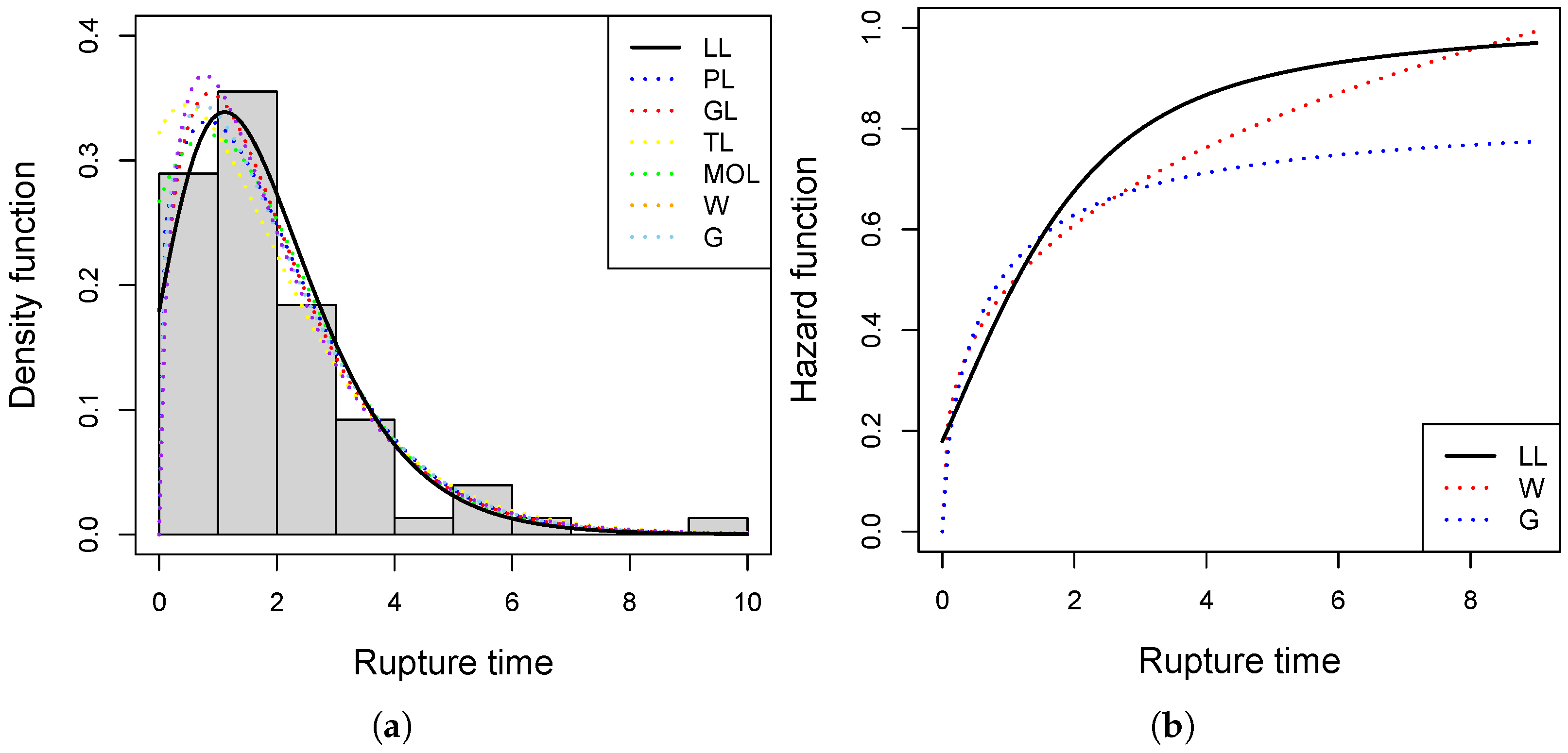
Figure 5 displays the rupture time data together with the fitted models. The left panel shows the histogram with the fitted PDFs. The LL distribution provides densities closer to the histogram frequencies, particularly around the modal region. The right panel compares the HRFs of the LL, W, and G distributions. The LL distribution exhibits a more sharply increasing hazard rate as rupture time increases, suggesting greater sensitivity to progressive system deterioration. In contrast, the W distribution shows a moderately increasing hazard, while the G distribution presents a smoother increase, underestimating the risk of failure at higher rupture times.

4.2. Hospital Stay Times Data

In the analysis of duration data in clinical contexts, it is essential to rely on distributional models flexible enough to adequately capture the strong skewness and dispersion typically exhibited by hospital stay times. In this type of data, a substantial proportion of observations correspond to short stays, while a smaller subset may present exceptionally long stays. This combination of frequent and extreme events generates positively skewed distributions with heavy tails, which are not well described by classical symmetric or light-tailed models.

In this application, we consider a dataset of 300 hospital stay times (in days) for patients diagnosed with breast cancer. Each observation represents the total number of days elapsed between hospital admission and medical discharge. These data were previously analyzed by Safari et al. [35] and are presented in

Table 6. Hospital stay times (in days) for 300 patients diagnosed with breast cancer.

8	4	3	30	15	54	24	7	4	21	5	7	3	12	26	2	61	9	11	26	12	20	60	4	24
2	12	9	36	14	12	37	35	21	11	7	2	7	33	13	25	33	11	26	31	13	26	12	22	9
21	4	8	10	2	48	30	17	6	7	15	6	12	19	13	15	5	10	7	22	26	15	55	7	5
9	6	11	10	26	24	37	7	3	16	26	15	9	16	13	11	7	2	9	10	10	20	9	7	17
19	26	7	2	11	7	8	15	6	4	21	5	13	13	37	2	8	7	16	11	15	25	8	3	10
21	10	11	4	29	28	13	10	15	20	60	12	10	3	51	17	31	4	5	11	9	30	17	26	5
40	74	14	16	33	23	19	3	89	14	20	48	26	13	12	10	10	15	14	5	23	36	6	5	3
28	28	23	12	3	4	68	10	4	30	8	6	23	14	14	1	1	16	80	1	14	18	30	17	26
5	50	17	14	15	33	23	17	9	3	59	40	27	40	3	14	87	16	14	14	11	11	32	24	15
18	31	2	8	11	17	7	48	1	25	25	77	7	2	6	2	32	12	17	19	13	1	23	20	16
46	10	14	2	5	35	9	18	2	50	7	40	22	46	19	31	13	15	26	31	5	26	1	25	46
94	9	11	12	27	12	15	31	10	30	16	14	14	49	22	17	22	7	17	4	17	13	5	33	27

.

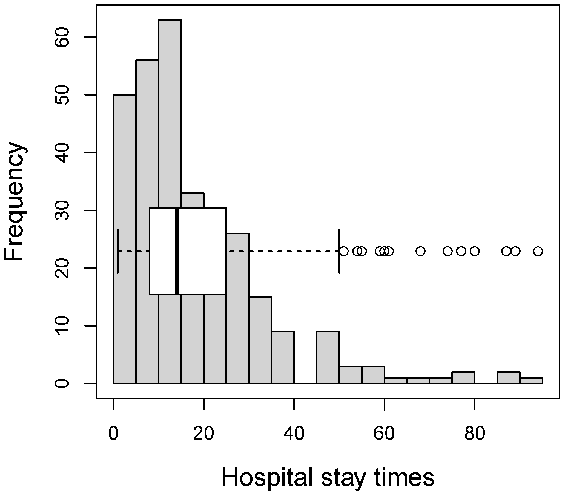
Some descriptive measures for these data are: mean 18.44, standard deviation 15.89, skewness coefficient 1.96, and kurtosis coefficient 7.91. These values indicate substantial variability and strong positive skewness, as well as heavy-tailed behavior due to the presence of outliers. This pattern is also reflected in Figure 6, where the histogram shows unimodality with a large concentration of stays shorter than 20 days, while the boxplot highlights a few extremely long hospitalizations.

Table 7. ML estimates with standard errors in parentheses, p-values from AD and CvM goodness-of-fit tests, and AIC and BIC values for each distribution fitted to hospital stay times data.

Parámetros	LL	MOL	G	TL	PL	GL	W
$\theta$	0.066	0.075	1.555	0.082	0.129	0.097	1.255
	(0.013)	(0.010)	(0.116)	(0.007)	(0.014)	(0.006)	(0.054)
$\alpha$	0.243	0.452	11.846	0.560	0.925	0.893	19.907
	(0.180)	(0.140)	(1.039)	(0.179)	(0.034)	(0.074)	(0.967)
AIC	2319.1	2320.2	2321.4	2321.8	2324.3	2326.9	2328.2
BIC	2326.5	2327.6	2328.8	2329.2	2331.7	2334.3	2335.6
AD	0.798	0.674	0.524	0.516	0.474	0.332	0.244
CvM	0.809	0.649	0.515	0.561	0.491	0.339	0.281

summarizes the ML estimates (with standard errors), together with p-values from the AD and CvM tests and the AIC and BIC criteria for all fitted models. The LL distribution clearly stands out by achieving the highest goodness-of-fit p-values and the lowest information criteria, thereby emerging as the most suitable model for these data.

Applying the Wald test analogously to the analysis conducted in Section 4.1, we tested the null hypothesis $H_0:\alpha =1$ for the hospital stay time data. Using the ML estimate $\widehat{\alpha }=0.243$ and its standard error $0.180$, the test statistic $W={\left[(\widehat{\alpha }-1)/\mathrm{se}\left(\widehat{\alpha }\right)\right]}^2=17.687$, which follows a ${\chi }_1^2$ distribution, resulted in a p-value smaller than $0.001$. This indicates that the parameter $\alpha$ significantly differs from one, providing statistical evidence that the LL distribution offers a substantially better fit than the classical L model.

Figure 7 provides a graphical comparison of the fitted models. The left panel shows the histogram of hospital stay times together with the fitted PDFs. The LL distribution provides a closer fit to the empirical frequencies, capturing both the main peak and the heavy right tail. The right panel displays the hazard rate functions of the LL, W, and G distributions. The LL distribution exhibits a sharper increase at early times followed by stabilization, reflecting greater sensitivity to the concentration of short stays and the occurrence of longer hospitalizations. In contrast, the W distribution shows a more gradual increase, while the G distribution yields an even smoother hazard, underestimating the probability of longer stays.

5. Final Comments

The Lambert–Lindley (LL) distribution introduced in this paper provides a flexible alternative for modeling positive, skewed, and unimodal data. Its formulation, based on the application of the Lambert-F generator to the Lindley (L) distribution, introduces an additional parameter that improves the ability of the distribution to capture varying levels of skewness and kurtosis.

Fundamental structural forms (including the probability density, distribution, quantile, and hazard rate functions) were derived, along with expressions for moments, measures of variability, and shape coefficients. These results indicate that the LL distribution overcomes the limitations of the classical L distribution by accommodating both unimodal and decreasing shapes, thereby offering greater versatility for analyzing data with different tail behaviors.

An important feature is the behavior of the PDF of the LL distribution at the lower bound of the support. Depending on the value of the shape parameter induced by the generator, the density in this region can be either higher or lower than that of the classical L distribution. This property enhances the ability to adequately model the lower quantiles, which is particularly relevant in applications that require describing short-duration phenomena or data with strong concentration near small values.

The analysis of the hazard rate function further showed that the LL distribution represents a modification of the classical L hazard rate at early times of the support. Depending on the value of the additional parameter, the hazard rate may lie above or below that of the L distribution in this initial region, thereby enabling a more accurate modeling of phenomena where early risk is relevant. In the long run, both distributions exhibit a similar asymptotic behavior, ensuring consistency in interpretation. This property enables the LL distribution to accommodate both monotonic hazard rates (different from those of the classical L) and non-monotonic shapes, broadening its applicability in reliability and survival analysis.

Parameter estimation was addressed using the method of moments and maximum likelihood, both requiring numerical procedures. A Monte Carlo simulation study confirmed the consistency and good performance of the estimators under different scenarios, thereby supporting their practical relevance.

In the applied setting, analyses with real datasets showed that the LL distribution can provide a better fit than widely used two-parameter models such as Gamma, Weibull, and several extensions of the L distribution. These results indicate that the new distribution is not only of theoretical interest but also offers tangible advantages in reliability engineering, healthcare, and other fields where modeling lifetimes or non-negative variables is required.

Beyond these numerical improvements, the LL distribution demonstrates practical relevance in real-world contexts such as reliability engineering, material fatigue, and environmental lifetime studies, where failure times or degradation processes often exhibit asymmetric patterns and non-constant risks. Its ability to capture both short-duration and long-tailed behaviors allows practitioners to represent systems with early failures, variable stress conditions, or lifetime dispersion driven by environmental or operational uncertainty. Therefore, the LL distribution extends beyond numerical superiority, providing a theoretically grounded and interpretable framework for modeling positive lifetime data observed in diverse applied disciplines.

Finally, a repository with the main functions and analyses developed in this study is made available.

References

1. Meeker, W.Q.; Escobar, L.A.; Pascual, F.G. Statistical Methods for Reliability Data; John Wiley & Sons: Hoboken, NJ, USA, 2021. [Google Scholar]
2. Collett, D. Modelling Survival Data in Medical Research; Chapman and Hall/CRC: London, UK, 2023. [Google Scholar]
3. Lancaster, T. The Econometric Analysis of Transition Data; Number 17; Cambridge University Press: Cambridge, UK, 1990. [Google Scholar]
4. Coles, S.; Bawa, J.; Trenner, L.; Dorazio, P. An Introduction to Statistical Modeling of Extreme Values; Springer: Berlin/Heidelberg, Germany, 2001; Volume 208. [Google Scholar]
5. Lindley, D.V. Fiducial distributions and Bayes’ theorem. J. R. Stat. Soc. Ser. B (Methodol.) 1958, 20, 102–107. [Google Scholar] [CrossRef]
6. Corless, R.M.; Gonnet, G.H.; Hare, D.E.G.; Jeffrey, D.J.; Knuth, D.E. On the Lambert W function. Adv. Comput. Math. 1996, 5, 329–359. [Google Scholar] [CrossRef]
7. Jodrá, P. Computer generation of random variables with Lindley or Poisson–Lindley distribution via the Lambert W function. Math. Comput. Simul. 2010, 81, 851–859. [Google Scholar] [CrossRef]
8. Ghitany, M.E.; Atieh, B.; Nadarajah, S. Lindley distribution and its application. Math. Comput. Simul. 2008, 78, 493–506. [Google Scholar] [CrossRef]
9. Johnson, N.L.; Kotz, S.; Balakrishnan, N. Continuous Univariate Distributions, Volume 1, 2nd ed.; Wiley-Interscience: New York, NY, USA, 1994. [Google Scholar]
10. Weibull, W. A Statistical Distribution Function of Wide Applicability. J. Appl. Mech. 1951, 18, 293–297. [Google Scholar] [CrossRef]
11. Zakerzadeh, H.; Dolati, A. Generalized Lindley Distribution. J. Math. Ext. 2009, 3, 13–25. [Google Scholar]
12. Ghitany, M.E.; Al-Mutairi, D.K.; Balakrishnan, N.; Al-Enezi, L. Power Lindley distribution and associated inference. Comput. Stat. Data Anal. 2013, 64, 20–33. [Google Scholar] [CrossRef]
13. Ghitany, M.E.; Alqallaf, F.; Al-Mutairi, D.K.; Husain, H.A. A two-parameter weighted Lindley distribution and its applications to survival data. Math. Comput. Simul. 2011, 81, 1190–1201. [Google Scholar] [CrossRef]
14. Merovci, F. Transmuted Lindley Distribution. Int. J. Open Probl. Comput. Sci. Math. (IJOPCM) 2013, 6, 63–72. [Google Scholar] [CrossRef]
15. Marshall, A.W.; Olkin, I. A new method for adding a parameter to a family of distributions with application to the exponential and Weibull families. Biometrika 1997, 84, 641–652. [Google Scholar] [CrossRef]
16. Eugene, N.; Lee, C.; Famoye, F. Beta-normal distribution and its applications. Commun. Stat.-Theory Methods 2002, 31, 497–512. [Google Scholar] [CrossRef]
17. Zografos, K.; Balakrishnan, N. On families of beta-and generalized gamma-generated distributions and associated inference. Stat. Methodol. 2009, 6, 344–362. [Google Scholar] [CrossRef]
18. Shaw, W.T.; Buckley, I.R. The alchemy of probability distributions: Beyond Gram-Charlier expansions, and a skew-kurtotic-normal distribution from a rank transmutation map. arXiv 2009, arXiv:0901.0434. [Google Scholar]
19. Cordeiro, G.M.; De Castro, M. A new family of generalized distributions. J. Stat. Comput. Simul. 2011, 81, 883–898. [Google Scholar] [CrossRef]
20. Mahdavi, A.; Kundu, D. A new method for generating distributions with an application to exponential distribution. Commun. Stat.-Theory Methods 2017, 46, 6543–6557. [Google Scholar] [CrossRef]
21. Iriarte, Y.A.; de Castro, M.; Gómez, H.W. The Lambert-F distributions class: An alternative family for positive data analysis. Mathematics 2020, 8, 1398. [Google Scholar] [CrossRef]
22. Iriarte, Y.A.; de Castro, M.; Gómez, H.W. An alternative one-parameter distribution for bounded data modeling generated from the Lambert transformation. Symmetry 2021, 13, 1190. [Google Scholar] [CrossRef]
23. Iriarte, Y.A.; de Castro, M.; Gómez, H.W. A unimodal/bimodal skew/symmetric distribution generated from Lambert’s transformation. Symmetry 2021, 13, 269. [Google Scholar] [CrossRef]
24. Varela, H.; Rojas, M.A.; Reyes, J.; Iriarte, Y.A. An alternative Lambert-type distribution for bounded data. Mathematics 2023, 11, 667. [Google Scholar] [CrossRef]
25. Gemeay, A.M.; Karakaya, K.; Bakr, M.; Balogun, O.S.; Atchadé, M.N.; Hussam, E. Power Lambert uniform distribution: Statistical properties, actuarial measures, regression analysis, and applications. AIP Adv. 2023, 13, 095319. [Google Scholar] [CrossRef]
26. Astorga, J.M.; Iriarte, Y.A. The Lambert-Topp-Leone distribution: An alternative for modeling proportion and lifetime data. Front. Appl. Math. Stat. 2025, 11, 1527833. [Google Scholar] [CrossRef]
27. Soetaert, K. rootSolve: Nonlinear Root Finding, Equilibrium and Steady-State Analysis of Ordinary Differential Equations, R package version 1.6; 2009. Available online: https://cran.r-project.org/web/packages/rootSolve/rootSolve.pdf (accessed on 1 October 2025).
28. Byrd, R.H.; Lu, P.; Nocedal, J.; Zhu, C. A limited memory algorithm for bound constrained optimization. SIAM J. Sci. Comput. 1995, 16, 1190–1208. [Google Scholar] [CrossRef]
29. Adler, A. lamW: Lambert-W Function, R package version 2.2.3; 2015. Available online: https://cran.r-project.org/web/packages/lamW/index.html (accessed on 1 October 2025).
30. Akaike, H. A new look at the statistical model identification. IEEE Trans. Autom. Control 1974, 19, 716–723. [Google Scholar] [CrossRef]
31. Schwarz, G. Estimating the dimension of a model. Ann. Stat. 1978, 6, 461–464. [Google Scholar] [CrossRef]
32. Faraway, J.; Marsaglia, G.; Marsaglia, J.; Baddeley, A. goftest: Classical Goodness-of-Fit Tests for Univariate Distributions, R package version 1.2-3; 2021. Available online: https://cran.r-project.org/web/packages/goftest/goftest.pdf (accessed on 1 October 2025).
33. Ghitany, M.; Al-Mutairi, D.; Al-Awadhi, F.; Al-Burais, M. Marshall-Olkin extended Lindley distribution and its application. IJAM Int. J. Appl. Math. 2012, 25, 709–721. [Google Scholar]
34. Andrews, D.; Herzberg, A. Stress-rupture life of kevlar 49/epoxy spherical pressure vessels. In Data: A Collection of Problems from Many Fields for the Student and Research Worker; Springer: Berlin/Heidelberg, Germany, 1985; pp. 181–186. [Google Scholar]
35. Safari, M.A.M.; Masseran, N.; Abdul Majid, M.H. Robust reliability estimation for Lindley distribution—A probability integral transform statistical approach. Mathematics 2020, 8, 1634. [Google Scholar] [CrossRef]
Figure 1. (a) LL PDF curves when θ = 0.5 . (b) LL PDF curves when θ = 5 .
Mathematics 13 03480 g001
Figure 2. (a) LL HRF curves when θ = 0.5 . (b) LL HRF curves when θ = 5 .
Mathematics 13 03480 g002
Figure 3. Plots of the coefficient of variation, skewness, and kurtosis for the LL distribution.
Mathematics 13 03480 g003
Figure 4. Histogram and boxplot for rupture time data.
Mathematics 13 03480 g004
Figure 5. (a) Histogram of rupture times with the fitted PDFs. (b) HRFs of the LL, W, and G distributions fitted to the rupture time data.
Mathematics 13 03480 g005
Figure 6. Histogram and boxplot for hospital stay data.
Mathematics 13 03480 g006
Figure 7. (a) Histogram of hospital stay times with the fitted PDFs. (b) HRFs of the LL, W, and G distributions fitted to the hospital stay times data.
Mathematics 13 03480 g007