A Vehicle Routing Problem Based on a Long-Distance Transportation Network with an Exact Optimization Algorithm

Abstract

In vehicle routing problems, long-distance transportation poses a significant challenge to the optimization of transportation costs while adhering to regulations. This study investigates a special type of logistics problem that focuses on liquid transportation systems involving full truckload delivery and the rest–break–drive periods of truck drivers over long distances according to the regulations of the United States. Based on an exact solution algorithm, this work combines a long-distance full truckload fluid transportation problem with the concept of truck driver schedules for the first time. The goal is to optimize transportation expenses while managing challenges related to the rest–break–drive periods of truck drivers, time windows, trailer varieties, customer segments, food and non-food products, a diverse fleet, starting locations, and the diverse tasks of vehicles. In order to reach optimality, a construction heuristic and the column generation method were employed, supplemented by several acceleration strategies. Performance analysis, carried out with artificial input sets mirroring real-life scenarios, indicates that low optimality gaps can be obtained in an appropriate amount of time for large-scale long-haul liquid transportation.

1. Introduction

The vehicle routing problem (VRP) is a fundamental problem in logistics and combinatorial optimization that involves determining the most efficient set of routes for a fleet of vehicles to deliver goods or services to a set of geographically dispersed customers. VRPs encompass numerous variants (examine the study of Konstantakopoulos et al. [1] for details), each of which requires a distinct solution approach, creating significant logistical challenges. Full truckload (FTL) delivery accounts for an important proportion among the VRP variants and it is aimed at transporting large-scale shipments exploiting maximum capacity. Today’s FTL systems can encompass a wide range of transportation options such as containers, cement, and liquid. Furthermore, the healthcare sector can explore the implementation of FTL principles by utilizing ambulance fleets to transport and deliver patients.

The FTL problem involves a network where a mixed fleet of rented and owned vehicles, equipped with different trailer types, is stationed at multiple depots. Vehicles transport products from supply (load) locations to customer (unload) locations, must return to the garage upon completing their routes, and are subject to time-window constraints. Trailer cleaning is required at washing centers when switching product types, with durations specified by a washing matrix. Product–trailer compatibility is determined by a trailer–product matrix. In practice, contracted customer demands are mandatory and prioritized, while non-contracted orders are optional and occur less frequently. When long distances between customer locations occur, a truck driver needs to rest or take a break in line with the legal rules enforced by regulators. In short, the rest, break, and drive periods of drivers should be arranged accordingly without violating those rules. Therefore, the main goal is to find optimal routes for the existing fleet by reducing total transportation expenses within the constraints associated with FTL operations.

The inclusion of various time frames, starting points, different customer categories, a mixed fleet, and washing activities greatly expands the range of factors that logistics companies need to consider. These factors exacerbate route complexity and make optimal vehicle decisions exceedingly challenging. In addition, truck driver schedules exacerbate the complexity further because determining the optimal combination and duration of rest, break, and drive periods escalates computational efforts tremendously. Even exploring a feasible solution becomes tougher. As a result, making suboptimal decisions within these combinations could result in increased fixed/variable costs on routes and dissatisfied clients. Consequently, a logistics company may suffer significant losses in profits, market share, and demand.

Given the intricate nature of VRPs, a variety of heuristic algorithms and their adaptations, including genetic algorithms (Holland [2]), ant colony algorithms (Dorigo et al. [3]), large neighborhood search algorithms, tabu search algorithms (Glover [4]), greedy randomized adaptive search (Feo et al. [5]), and variable neighborhood search (Mladenović et al. [6]), are extensively used to create initial solutions and enhance them as needed. However, these algorithms are not intended to ensure optimal solutions. Instead, they simply offer upper bounds for the relevant problem. Given that scheduling constraints already make finding a feasible solution difficult, enhancing the established solution also presents challenges in terms of heuristics.

Exact algorithms are not as commonly used in VRPs as heuristic methods. The application of exact algorithms for FTL concepts is very uncommon, as FTL problems have not been extensively researched in the VRP field. This work integrates both exact algorithmic methods and heuristic approaches to solve this particular FTL issue. A construction heuristic (Solomon, [7]) is used to create first routes/columns to start off the exact algorithm that follows the column generation (CG) method’s rules, as outlined by Dantzig and Wolfe [8].

Arc flow inequalities (Costa et al. [9]) and k-path inequalities (Desaulniers et al. [10]) are included to contribute to reducing the optimality gap and bolster the CG algorithm by creating promising paths using various dual variables. Moreover, distinct concepts are implemented to speed up the CG iterations. The initial acceleration method, pioneered by Righini and Salani [11], involves a bi-directional exploration for path generation. The second method incorporates ng-route relaxation, pioneered by Baldacci et al. [12], enabling the incorporation of non-elementary paths (no cycle exists) alongside elementary ones in the relaxed master problem of the column generation algorithm. The third method concentrates on prioritizing subproblems likely to include favorable columns/routes. While mainly heuristic, this method is capable of assessing all subproblems when needed. The last method, inspired by Desaulniers et al. [10], detects the first promising column derived within the current subproblem. Despite its heuristic nature, this method can also consistently assess all possible paths to provide thorough exploration.

In a nutshell, this study analyzed a long-distance FTL network that commonly occurs in the logistics market. Our contributions can be summarized as follows:

• The United States’ regulatory framework governing rest, break, and driving periods is uniquely integrated with a logistics environment characterized by multiple product and trailer categories, several departure locations, multiple time windows of nodes, a heterogeneous vehicle fleet, and a constrained number of available vehicles.
• A unique enhancement has been introduced to the considered FTL network specifically aiming to reinforce road safety and safeguard driver well-being in the context of long-haul transportation.
• This study seeks to determine the optimal timing and duration of breaks and rest periods along the routes for the specified FTL network while optimizing total transportation cost.
• The column generation operations for the specified FTL problem are distinctively integrated with a rest–break–drive policy, enabling the explicit incorporation of regulatory driving constraints into the optimization process.
• A rest–break–drive policy is uniquely combined with the acceleration strategies incorporated into the column generation procedure for the specified FTL problem, thereby enhancing the rate of convergence toward the optimal solution of the relaxed master problem.
• With the integrated consideration of truck driver scheduling constraints, this research undertakes an extensive performance evaluation of the proposed algorithm, encompassing a broad spectrum of scenarios for the specified FTL framework.

After Section 1, Section 2 introduces important works in the literature, specifically focusing on FTL transportation systems with truck driver scheduling. Section 3 outlines the problem definition and mathematical formulation and visualizes the network flow of vehicles. Following that, Section 4 discusses crucial parts of the whole algorithm whereas Section 5 presents its performance for the corresponding inputs. Lastly, Section 6 offers a conclusion and explores favorable future research avenues.

2. Literature Review

Frankly, there is an insufficient number of studies regarding FTL networks in the literature. Whereas a few works explore the FTL concept, its importance in supply chain systems is evident. Existing research mainly focuses on heuristic algorithms for specific problems with few solutions based on exact algorithms. Recent advancements in techniques like machine learning and simulations have been applied to VRPs, but there is a lack of studies integrating these approaches with exact algorithm enhancements, especially in the context of FTL problems. Our study aims to address this gap by combining exact and heuristic approaches with acceleration methods.

The FTL problem was initially presented by Ball et al. [13] with the objective of determining the optimal fleet size through the creation of vehicle routes that adhere to maximum route-time constraints. They successfully identified the issue and suggested some potential solutions to tackle the key implementation challenges. Then, Desrosiers et al. [14] employed an asymmetrical traveling salesman problem with two types of constraints to demonstrate its effectiveness in FTL systems.

It can be observed that the literature covers many heuristic algorithms applied to FTL problems due to their ease of implementation and polynomial time complexity as opposed to exact algorithms. However, when searching for studies on truck driver scheduling constraints in FTL transportation, studies become significantly fewer with respect to both heuristic and exact algorithms. Particularly, exact algorithms based on driver scheduling in VRPs are still an emerging concept due to the fact that the first relevant studies were introduced by Tilk [15] and Goel and Irnich [16] under United States regulations. Afterwards, Tilk and Goel [17] expanded the previous works to include acceleration techniques as well as European Union regulations. The rest, break, and drive periods of drivers were integrated during the solution process of those two studies.

Mayerle et al. [18] investigated a long-haul FTL system and truck driver scheduling problem with intermediate stops based on Brazilian policy. Refueling, rest, and drive periods were included in the mixed-integer modeling of the problem, merging a state space graph search approach. Alireza et al. [19] focused on time slot management in a selective pickup–delivery problem with mixed time windows, as in the operations of FTL systems. A set of valid inequalities was employed to reinforce the mixed-integer linear programming performance under both hard and soft time windows. De Genaro et al. [20] focused on state space shortest path heuristics to solve a long-haul point-to-point vehicle routing and driver scheduling problem subject to hours of regulatory service constraints. Stoppage alternatives such as quick rests, weekly drive periods, meals, and overnight rests were included as well. However, it is devoid of exact algorithm approaches as well as a heterogeneous fleet, multiple trailer types and departure nodes. Also, no washing action takes place, as opposed to our work. Sartori et al. [21] investigated the scheduling of truck drivers with independent routes under European Union regulations. Mixed-integer programming was used to involve driver scheduling constraints as well as operational constraints such as load transfers between two vehicles at cross-dock or transfer locations and time windows, as in point-to-point transportation. Chen et al. [22] examined an integrated scheduling of zone picking and delivery problem based on FTL operations. Mixed-integer modeling was deployed to reach optimal solutions for scheduling setup times and driving times between zones. Eskandarzadeh et al. [23] studied rest and break policy comparisons for heavy vehicles in Australia, encompassing a pickup and delivery approach. In order to solve this pickup-and-delivery-oriented problem, a mixed-integer modeling technique was used to acquire optimal routes respecting rest and break policies. Xu et al. [24] focused on truck routing and platooning optimization considering drivers’ mandatory breaks based on pickup and delivery operations. Novel mixed-integer programming techniques and iterated neighborhood search were employed to tackle the problem. Mor et al. [25] examined a bi-objective long-haul transportation problem on a network involving rest periods for drivers and fueling periods of the vehicle. Minimization of fuel cost and path duration was an aim during point-to-point transportation. Lucci et al. [26] studied a metaheuristic for crew scheduling in a pickup–delivery problem with time windows. Long-distance FTL transportation was analyzed over a multi-day planning horizon including multiple time windows and hours of service regulations. Although there are some common points with our work, Lucci et al.’s study is not even an exact-algorithm-oriented study. In addition, due to the fact that no liquid transportation exists in their study, they lack multiple trailer types and washing operations as well. Garaix et al. [27] designed a label-setting algorithm for a truck driver scheduling problem considering European Community social legislation. Minimization of completion time over a given order of nodes with FTL or LTL transportation was achieved by incorporating drivers’ break and rest periods. Emre and Erol [28] conducted a study on a liquid-transportation-based FTL network that focuses on varied departure times of vehicles to minimize redundant waiting times en route as well as transportation expenses. They employed a column generation approach for the exact solution. However, their work lacks consideration of driver schedules, which must be taken into consideration during trips over long distances due to government regulations. With respect to the drivers, knowing when to take breaks or rests and how much time to allocate for breaks or rests while obeying regulations and satisfying customers is significant. If regulations are breached, huge fines are imposed by traffic control policies and transportation becomes unsafe, increasing the chance of accidents. It must also be expressed that there is actually a nested label-setting algorithm in our work as opposed to in Emre and Erol’s [28], which includes an unnested one. This is because, in Emre and Erol [28], labels are updated only when a subsequent node is visited. However, in our work, labels are computed during travel between two nodes. For example, whenever a break is needed during travel, labels are updated. If a period of driving takes place after that break, then labels are updated again. If a rest is needed after that driving period, then labels are updated once more. Thus, in our work, many label calculations have to take place even before a driver visits the chosen node due to the possible combinations of break–rest–drive periods during travel towards that node. Furthermore, because of the fact that the column generation method is a frame and heavily problem-dependent, completely different labels and labeling procedures should be taken into account with regard to distinct problem concepts. Therefore, this situation distinguishes our work from Emre and Erol’s [28] considerably. Danach [29] employed a reinforcement learning technique to address challenges in demand pattern prediction and real-time identification of efficient routes, enabling dynamic adjustments in response to sudden changes in traffic congestion or demand. He worked on a capacitated vehicle routing problem with time windows through comparisons of mixed-integer modeling and some heuristic algorithms. Kadyrov et al. [30] presented detailed comparisons between metaheuristic algorithms and reinforcement learning algorithms, some of which were merged with heuristic methods, to find satisfactory solutions. They worked on a just capacitated vehicle routing problem through comparisons between some critical heuristic algorithms.

According to the literature, many exact algorithms that involve FTL operations and truck driver scheduling lack efficient CG methods when dealing with large-scale instances. To the best of our knowledge, no study has focused on long-distance liquid transportation-based FTL systems with truck driver scheduling. The novel aspects of our work can be seen summarized in

Table 1. Comparison of some studies in the literature based on critical aspects.

Studies	A	B	C	D	E	F	G	H	I	J	K
Mayerle et al. [18]	X	X			X	X				X
Tilk, Goel [17]	X	X	X								X
Goel, Irnich [16]	X	X	X								X
De Genaro et al. [20]		X			X	X				X
Sartori et al. [21]	X	X		X	X
Chen et al. [22]	X	X		X		X				X
Eskandarzadeh et al. [23]	X	X				X				X
Mor et al. [25]	X	X
Garaix et al. [27]	X	X			X	X				X
Lucci et al. [26]		X		X	X	X	X			X
Our Work	X	X	X	X	X	X	X	X	X	X	X

below. Therefore, our work aims to achieve optimal routing and scheduling for drivers using a CG-based exact algorithm along with its acceleration techniques and a construction heuristic algorithm with the incorporation of the mentioned FTL network structure.

In terms of Table 1, A–K imply A: exact algorithm solution; B: truck driver scheduling; C: column-generation-based exact method; D: multiple departure nodes; E: multiple time windows; F: multiple product types; G: heterogeneous fleet; H: multiple trailer types; I: washing of trailers; J: FTL transportation; and K: truck driver policy under United States regulations.

3. Problem Description

3.1. Problem Definition

The work focuses on an optimal solution for a truck driver scheduling problem involving full truckload deliveries. The problem includes multiple departure nodes/points, as vehicles may be in idle positions in different locations before their journey starts. In addition, vehicles should return to a garage after their jobs are finished, which is why the problem has a single terminal node/point. Various time window constraints are included to be able to serve customer nodes in different time intervals. The fleet size is always finite, therefore a finite number of vehicles are involved for each type. Distinct vehicle and trailer categories and different product types are also embedded into the problem as required by the logistics sector. Also, not all customer nodes are similar to each other because contracted and non-contracted customer types matter to a logistics company in real life, which is why there is a combination of these customer types. Contracted customers’ orders must be satisfied. However, non-contracted customers’ orders may not be fulfilled if they do not reduce overall costs. Each time window at a node represents a separate time interval. In fact, our work has hard time windows instead of soft ones, which means if a vehicle arrives early with respect to a specified window, then it is forced to wait until the opening of its specified time window. If a vehicle arrives late, it may not be able to service during that time window. In addition, logistics firms may combine requests for future service in order to reduce costs by considering various time windows for pickup locations (supply zones) and delivery locations (demand zones), which expands the range of possible route options to meet customer needs while adhering to their deadlines. For example, customers may request to receive their order within a maximum of four days. This is why our study includes multiple daily time windows.

Furthermore, FTL systems generally involve vehicles which are located at multiple starting points with a trailer after completing their previously assigned routes based on prior demands. These vehicles add complexity to the problem, as decisions need to be made with regard to their starting points. The problem involves a finite number of vehicles, which are divided into two different categories and allocated to each departure zone. It must be discerned that firms frequently lease extra vehicles to reduce transportation expenses. However, in spite of the benefits, these companies must still sustain their own fleet to minimize dependence on these leasing firms. Therefore, effective usage of the fleet is rather significant.

Product compatibility is a crucial factor to consider in FTL actions due to contamination issues. For example, in liquid food transportation, a vehicle may have transported glucose syrup previously and may be assigned to transport canola oil subsequently. Therefore, the trailer must be exposed to a washing process before the loading of canola oil to alleviate contamination problems. Thus, trailer–product and washing matrices were built to respect contamination constraints. According to the first matrix, one can observe whether a corresponding trailer can transport corresponding products, whereas the second matrix indicates the duration of the washing process to ensure the switch between two products for a trailer.

In addition, FTL actions always encompass many varying tasks for vehicles. For example, a vehicle is always required to load a product and unload it subsequently in FTL transportation. Supply nodes are generally conceived as loading zones while demand nodes are conceived as unloading zones. Therefore, in this study, demand nodes are customer points where demands are met, while supply nodes allow logistics firm to load relevant products from their location and carry them to their customers.

Finally, due to long distances, truck drivers are required to take a rest or break after a certain period of time to ensure safe transportation. Redundant waiting times, long driving periods, and processing times can decrease the energy of drivers. Therefore, drivers should obey the rules set by regulators. Nevertheless, rest and break periods have a minimum duration when they are needed. Therefore, a driver can extend their break or rest period to eliminate or reduce waiting times during the visit of a node. This way, the driver can preserve their energy more effectively.

The goal is to minimize overall transportation expenses while keeping the optimality gap low, within acceptable computational limits, as well as providing the best routes for the designated vehicles with scheduled driver periods.

Based on the definition provided above, the key features of the associated FTL concept are outlined below:

• Drivers cannot drive while violating break and rest rules imposed by regulations.
• Drivers can prolong only last rest or last break periods to reduce waiting times.
• Drivers can exceed the maximum permissible time without any rest or break period during waiting times or processing times at nodes.
• Drivers cannot take partial rest or break periods.
• Every designated rest period inherently constitutes a break.
• Break periods cannot be regarded as a rest period.
• There can be no consecutive rest period after a break period
• There can be no consecutive break period after a rest period
• Accumulated durations of being on break, driving, waiting, and operational processing activities progressively contribute to driver fatigue, thereby mandating rest periods at subsequent stages of the schedule.
• Prolonged driving, waiting, and operational processing activities similarly lead to driver fatigue, necessitating the enforcement of break periods in later stages.
• A delayed vehicle departure does not alter the driver’s initial rest or break allocation.
• No stringent regulation governs the latest allowable departure times at departure nodes.
• There are no prescribed requirements concerning the earliest permissible arrival times at garage/terminal nodes.
• The continuation of a driver’s schedule is contingent upon the selection of a corresponding feasible arc.
• There cannot be multiple drivers in one vehicle.
• The cost associated with rented vehicles for traversing each arc is lower than that of owned vehicles.
• Travel times regarding arcs can be higher or lower for rented vehicles compared to owned vehicles.
• The transportation network comprises washing nodes to ensure product transitions regarding trailers.
• The transportation network has multiple departure nodes for idle vehicles.
• The transportation network contains supply and demand nodes for loading and unloading, respectively.
• The transportation network includes a terminal node.
• Each product category has one supply node as well as multiple demand nodes.
• Time windows exist for supply nodes/load zones, demand nodes/unload zones, and washing nodes, while departure nodes and the terminal node have only one time window.
• There is no processing time for departure nodes and garage nodes.
• Vehicles are rented or owned in the fleet.
• Predetermined varieties of trailers are suitable for carrying specific goods.
• When a trailer is forced to transport a distinct product, a washing operation should be imposed involving washing costs and time.
• Vehicles cannot change their trailers on their assigned routes.

The following assumptions have been made for the methodology:

• No upper limit, which is prescribed for the duration of cumulative operational processing activities at visited nodes between two break periods, is required.
• There is no stipulated maximum cumulative driving time between two break periods.
• Regulations do not mandate a compulsory overnight rest period for drivers.
• Regulatory frameworks do not stipulate obligatory break intervals for drivers to be taken at fixed times throughout the day.
• No allowances exist permitting the exceedance of total driving time limits within a week, month, or specified multi-day period on some occasions in terms of regulations.
• There is no provision for reducing the duration of rest or break periods occasionally within a week, month, or designated multi-day interval.
• Certain minimum required times for rest and break periods exist.
• A certain maximum drive time without any rest period is encompassed.
• A certain maximum elapsed time without any rest period exists.
• A certain maximum elapsed time without any break period exists.
• Upon the vehicle’s arrival at the garage node, the driver’s break or rest period is disallowed.
• At the departure location, all trailer types compatible with the specific product category associated with that departure point are accessible for use with each vehicle type.
• Traffic jams, accidents, or sudden perturbations of assigned routes are disregarded.
• Multiple time windows are separate, daily, consecutive, and limited.
• A restricted number of owned and rented vehicles are available at each starting point.
• The expense of arc traveling and washing operations are fixed in advance.
• There are specific revenues available for non-contracted customers upon vehicle arrival.
• The operations of loading and unloading can solely occur at designated supply and customer points, respectively.
• Trailers are the same except for their capability to transport different goods.
• The expense of transporting a loaded vehicle is twice as high as that of transporting an unloaded one.
• A set number of washing centers and supply, customer, and departure points are involved.
• Established travel and washing times are in place.
• The trailer–product and washing matrices stay same.
• A fixed number of product and trailer types are considered.

As can be seen, a significant portion of the assumptions concern truck driver scheduling; however, these assumptions are aligned with U.S. regulations rather than being arbitrarily imposed or tailored to our problem. Almost none of these assumptions would be directly applicable under EU regulations. For instance, not requiring a nighttime rest period may appear to be a simplification, yet it reflects a realistic condition since U.S. regulations do not mandate it. Indeed, transportation does not universally halt at night. Similarly, the requirement of a maximum cumulative processing time without breaks does not exist in U.S. rules but exists in EU rules. In addition, while weekly driving limits are present in EU regulations, they do not constitute a simplification here because such provisions are absent from U.S. regulations. Overall, most aspects disregarded by U.S. rules are explicitly covered by EU rules, which adopt a more protective stance toward drivers and emphasize both road and driver safety more than the U.S. In summary, the structures outlined in our assumptions are consistent with U.S. regulations but not with those of the EU. In fact, it can be put into words that we assume U.S. rules for the specified FTL problem in our work instead of the EU’s.

According to the United States’ driving rules, there is no weekly driving limit; however, there exists a weekly working limit, which encompasses both driving periods and processing times for the relevant nodes. Specifically, a driver may work for a maximum of 60 h within 7 consecutive days or 70 h within 8 consecutive days. In addition, U.S. driver regulations require a minimum rest period of 10 consecutive hours, either between two 11 h driving periods or between two 14 h non-rest periods. It should also be noted that our daily time horizon is a maximum of 4 days, equivalent to 96 h. Therefore, in the worst-case scenario, a driver can work at most 96 − 96/(14 + 10 + 14) × 10 = 70.74 h within 96 h. However, it is important to emphasize that the 14 h non-rest activity period cannot consist entirely of driving, since 11 h of driving requires a subsequent non-driving interval under U.S. regulations. Moreover, drivers are only engaged in processing activities at supply and demand nodes, as washing operations are performed by a separate team while the driver just waits. Nevertheless, a 14 h non-rest period cannot involve only processing times, given that each processing activity lasts at most an hour (due to activity at our supply and demand nodes) and a driver can perform only two consecutive one-hour processing activities in 14 h after a travel period of at least 9 h (our travel times between any two nodes range from 9 to 18 h). Hence, a 14 h non-rest period includes at most 11 h of driving and 2 h of processing, leaving at least 1 h of waiting or break time. If each 14 h period contains at least 1 h of waiting or break, then the upper bound of a driver’s total working time is 70.74 − 96/(14 + 10 + 14) × 2 × 1 = 65.68 h. Therefore, within a 4-day horizon, the specified FTL problem does not violate the regulation stipulating a maximum of 70 working hours within 8 consecutive days. For an extensive review of United States regulations related to property-carrying vehicles, https://www.fmcsa.dot.gov/ (accessed on 19 October 2025) can be visited.

It should be noted that rest and break periods can be regarded as memoryless situations. When a driver takes a rest, the route is resumed as if no fatigue had been accumulated, effectively constituting a fresh start with respect to rest-related constraints. Similarly, when a driver takes a break, some degree of fatigue remains; however, the driver’s energy is partially restored, allowing the route to continue as if no time had been spent exhausting energy under break-related constraints. More specifically, an extension of the last rest or break period is introduced to eliminate or reduce waiting times at node visits. Due to this memoryless structure, extending previous rest or break periods, other than the last one, has no practical relevance. For a comprehensive review, the study by Tilk and Goel [17] can be examined as well.

In our problem, each unit of time corresponds to a 30 min interval. As a result, the various time windows are established based on the operational hours at supply and customer nodes. Departure points and terminal points are exempt from time window restrictions. In addition, travel and processing times are modified to adhere to this time framework.

3.2. Mathematical Formulation

Initially, mathematical formulation depends on the column generation method pioneered by Dantzig and Wolfe [8]. In the VRP literature, small-scale and medium-scale problems can be solved using mixed-integer programming models. For medium-scale problems, additional efforts such as valid inequalities or cutting planes are generally involved to reduce the integral gap and alleviate the branch nodes of the mixed-integer programming model. For large-scale instances, heuristics are mostly integrated to find promising upper bound solutions. However, branch–price–cut (BPC) algorithms currently lead the way in obtaining optimality for large-scale VRPs in the literature due to the extremely efficient working principle of CG methods in VRP systems, as a result of the work by Desrosiers et al. [31].

The notation employed for the CG model in this study is displayed in

Table 2. Notation for the Mathematical Formulation.

Sets
$\mathit{C}$	all contracted customers
${\mathit{C}}^{\prime }$	all non-contracted customers
$\mathit{S}$	all suppliers
$\mathit{W}$	all washing nodes
$\mathit{D}$	all departure nodes
$\mathit{G}$	terminal node
$\mathit{J}$	all vehicle categories
$\mathit{O}$	all trailer categories
${\mathit{I}}_{\mathit{o}}$	all departure nodes where trailer type $o\in O$ can start its journey while $I_o\subseteq D$
$\mathit{K}$	all possible feasible routes
${\mathit{A}}^{\mathrm{\ast }}\left(\mathit{S}\mathit{C}\right)$	for each arc $\left(i,j\right)$, where $i\in S$ and $j\in C\bigcup C^{\prime }$, $A^{\mathrm{\ast }}\left(i,j\right)$ includes just $\left(i,j\right)$ if $(j,i)$ does not exist; otherwise, it includes both $\left(i,j\right)$ and $(j,i)$
${\mathit{A}}^{\mathrm{\ast }}\left(\mathit{C}\mathit{W}\right)$	for each arc $\left(i,j\right)$, where $i\in C\bigcup C^{\prime }$, and $j\in W$, $A^{\mathrm{\ast }}\left(i,j\right)$ includes just $\left(i,j\right)$ if $(j,i)$ does not exist; otherwise, it includes both $\left(i,j\right)$ and $(j,i)$
$\mathit{P}\left(\mathit{C}\right)$	all subsets, each of which comprises two contracted customers
${\mathit{A}}^{-}\left(\mathit{U}\right)$	inward arcs with respect to each $U\in P\left(C\right)$
Variables
${\mathsf{\theta }}_{\mathit{o}\mathit{i}\mathit{j}\mathit{k}}$	binary route variable
Parameters
${\mathit{a}}_{\mathit{o}\mathit{i}\mathit{j}\mathit{k}\mathit{q}}$	the number of times $q\in C$ is visited in ${\theta }_{oijk}$
${\mathit{a}}_{\mathit{o}\mathit{i}\mathit{j}\mathit{k}{\mathit{q}}^{\prime }}$	the number of times $q^{\prime }\in C^{\prime }$ is visited in ${\theta }_{oijk}$
${\mathit{b}}_{\mathit{o}\mathit{i}\mathit{j}\mathit{k}\mathit{m}\mathit{n}}$	the number of times an arc $\left(m,n\right)$ is covered in ${\theta }_{oijk}$
${\mathit{c}}_{\mathit{o}\mathit{i}\mathit{j}\mathit{k}}$	the transportation cost of ${\theta }_{oijk}$

below.

With respect to the notation table, the CG model was devised accordingly below.

$$min \sum _{o\in O}\sum _{i\in I_o}\sum _{j\in J}\sum _{k\in K}{c}_{oijk}{\theta }_{oijk}$$

(1)

subject to

$$\sum _{o\in O}\sum _{i\in I_o}\sum _{j\in J}\sum _{k\in K}{a}_{oijkq} \ast {\theta }_{oijk}=1, \forall q \in C$$

(2)

$$\sum _{o\in O}\sum _{i\in I_o}\sum _{j\in J}\sum _{k\in K}{a}_{oijk{q}^{\prime }} \ast {\theta }_{oijk}\le 1,\forall q^{\prime }\in C^{\prime }$$

(3)

$$\sum _{k\in K}{\theta }_{oijk}\le H_{oij }, \forall o\in O, \forall i\in I_o , \forall j\in J$$

(4)

$$\sum _{o\in O}\sum _{i\in I_o}\sum _{j\in J}\sum _{k\in K}\sum _{\left(m,n\right) \in A^{-}\left(U\right)}{b}_{oijkmn} \ast {\theta }_{oijk}\ge 2,\forall U \in P\left(C\right)$$

(5)

$$\sum _{o\in O}\sum _{i\in I_o}\sum _{j\in J}\sum _{k\in K}\sum _{\left(m,n\right) \in A^{ \ast }(m^{\prime },n^{\prime })}{b}_{oijkmn} \ast {\theta }_{oijk}\le 1,\forall \left(m^{\prime },n^{\prime }\right)\in A^{ \ast }\left(CW\right)$$

(6)

$$\sum _{o\in O}\sum _{i\in I_o}\sum _{j\in J}\sum _{k\in K}\sum _{\left(m,n\right) \in A^{ \ast }(m^{\prime },n^{\prime })}{b}_{oijkmn} \ast {\theta }_{oijk}\le 2,\forall \left(m^{\prime },n^{\prime }\right)\in A^{ \ast }\left(SC\right)$$

(7)

$$\begin{gathered} \mathrm{Each} {\theta }_{oijk} \mathrm{respects\; the\; truck\; driver\; constraints\; that\; are\; regulated\; by} \\ \mathrm{United\; States\; Federal\; Motor\; Carrier\; Safety\; Administration\; (an\; inherently} \\ \mathrm{challenging\; restriction,\; largely\; attributable\; to\; the\; elaborate\; interactions} \\ \mathrm{embedded\; within\; break–rest–drive\; dynamics.)} \end{gathered}$$

(8)

$${\theta }_{oijk} \mathrm{is} \mathrm{binary}, \forall o\in O, \forall i\in I_o , \forall j\in J,\forall k\in K$$

(9)

It is important to emphasize that solving the integer relaxation of the formulation given in (1)–(9) is challenging, primarily due to the considerable complexity introduced by Constraint (8). Nonetheless, this constraint can be excluded from the explicit model and instead merged implicitly by ensuring that each generated column or route inherently satisfies the truck driver scheduling requirements. Consequently, the integer-relaxed variant of the CG formulation, namely the relaxed master problem (RMP), can be addressed to obtain a valid lower bound for the optimal solution. Objective (1) aims to reduce transportation costs. Constraint (2) ensures that contracted customers are visited. These customers have priority and must be visited exactly once due to contractual obligations. Constraint (3) dictates that non-contracted customers should be selected based on profitability, limiting their multiple visits. Constraint (4) sets the maximum available number of rented and owned vehicles at each starting point for the relevant trailer. Constraint (5) belongs to k-path (k = 2) inequalities (Desaulniers et al. [10]). Additionally, all subsets $U\in P\left(C\right)$ were constructed to ensure that they do not have any intersection. Constraints (6) and (7) are arc flow constraints introduced by Costa et al. [9], whereas Constraint (9) is a binary constraint. To streamline the column generation process, cuts in Constraints (6) and (7) were introduced one by one after a specified number of columns are generated. This method enables the creation of distinct dual variables from different constraints, supporting the identification of optimal routes in the subproblem solutions.

In the VRP literature, it is important to highlight that k-path inequalities which were specifically developed to enhance the RMP in the context of the CG process lead to a reduction in the optimality gap of solutions. This enhancement allows for an improvement in the lower bound, ultimately yielding a reduction in the optimality gap. Desaulniers et al. [10] have demonstrated the significant improvement in the lower bound achieved by incorporating 2-path inequalities in CG methods. While it is possible to include k-path (k > 2) inequalities in the RMP to further reduce the optimality difference, the addition of a large number of constraints may slow down the solution process of the RMP. It is important to note that the simplex algorithm is utilized during the RMP iterations, and based on complexity analysis, it is not deemed to be an efficient algorithm. Hence, the introduction of many constraints could negatively impact the basis matrix iterations and hinder the execution of the RMP. Alternatively, interior point methods in convex optimization can also be applied to solve the RMP. However, a large number of constraints could again dramatically exacerbate the performance of the RMP’s solution. BPC algorithms prioritize 2-path inequalities over others (k > 2) because logic-based branching or network branching strategies (as discussed in Kohl et al. [32] and Kallehauge et al. [33]) have the ability to reduce the optimality gap considerably in relaxed master problems compared to k-path (k > 2) inequalities. In this study, no branching strategy is necessary because of the low optimality gap, as shown in Section 5.

An arc flow cut measures the flow over the specified arc, creating a valid inequality for the CG model (see Costa et al. [9] for an extensive review). This situation implies that the addition of these inequalities does not disrupt the optimal integer solution of the CG model; however, they are capable of increasing the lower bound of the RMP. Undoubtedly, particularly in large-scale instances, there are a tremendous number of arcs and adding all of the relevant arc flow constraints simultaneously to the RMP would cause a significantly slower convergence of the RMP. Therefore, an arc flow constraint for each arc should be added gradually. For example, in our study, these valid inequalities were progressively added every 50 iterations to manage them effectively.

3.3. Network Representation

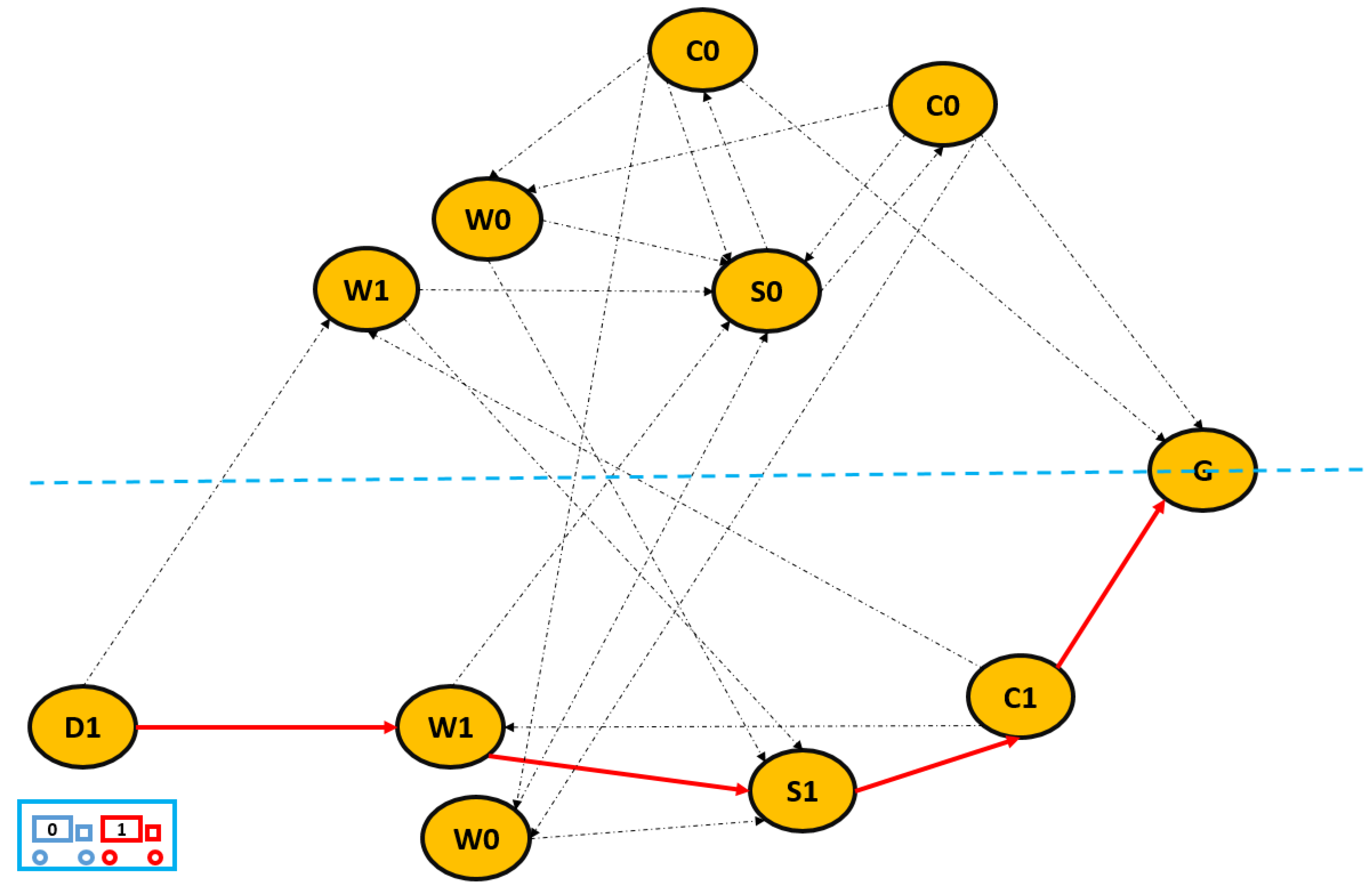
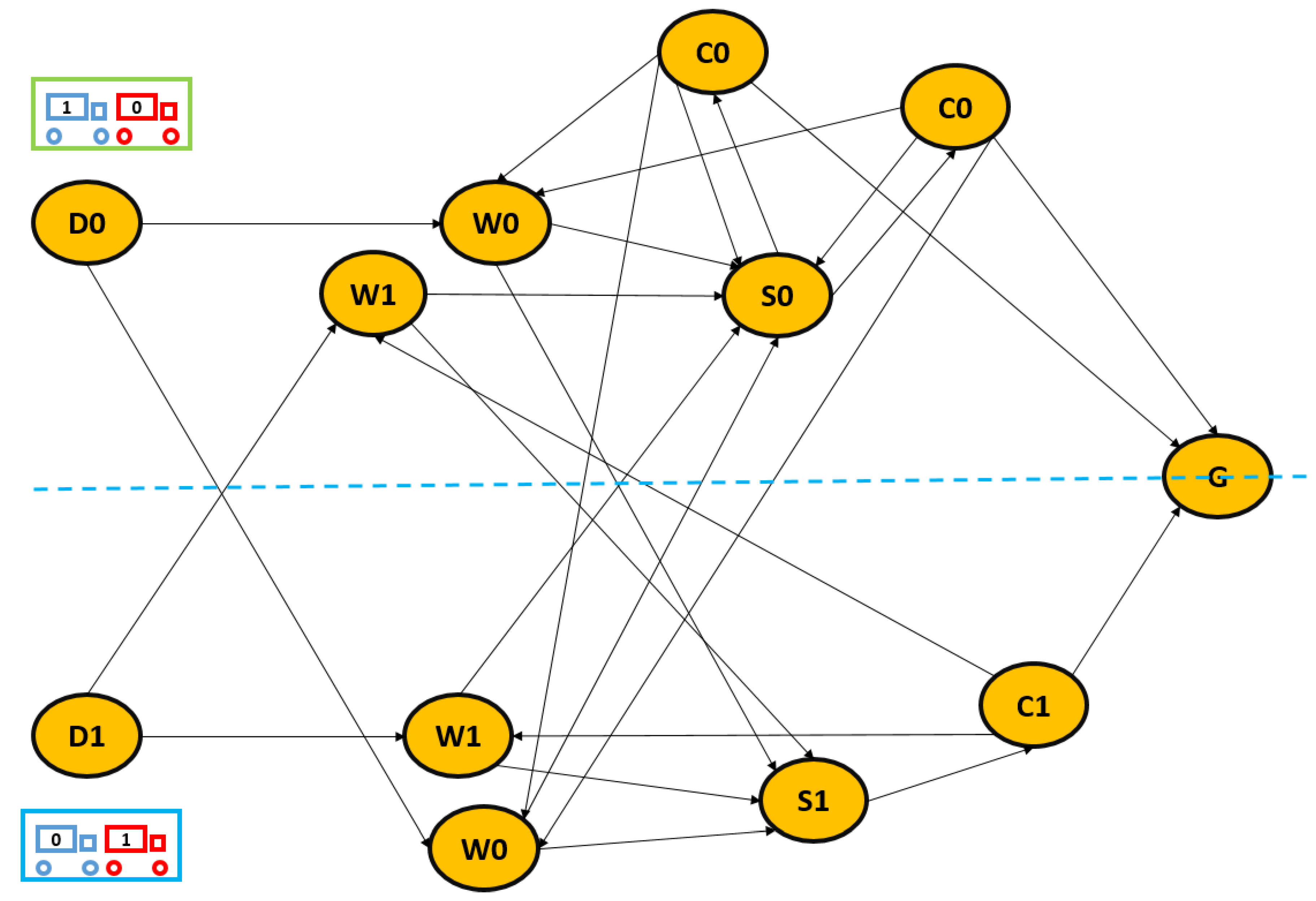
In this part, a simplified illustrative example is employed to clearly articulate the operational dynamics of the specific FTL problem under investigation, with a particular emphasis on elucidating the associated network structure. Thus, Figure 1 encapsulates the entirety of the problem’s structural framework. The figure depicts two distinct vehicles, a blue vehicle with a green trailer, representing the logistics company’s own vehicle, and a red vehicle with a blue trailer, symbolizing a rented vehicle. $W_i$ is the washing node for the $i^{th}$ product type and the $i^{th}$ product can only be washed at $W_i$. $D_i$ implies the starting point of vehicles that have just carried the $i^{th}$ product type at that time. $S_i$ is the supply node for the $i^{th}$ product type whereas $C_i$ is the customer node for the $i^{th}$ product type. Finally, $G$ represents the garage node.

According to Figure 2, it presents illustrative examples of both the washing matrix and the trailer–product compatibility matrix. In the washing matrix, each element denotes the time units required to convert a trailer from transporting one product category to another. Conversely, each element of the trailer–product matrix specifies the feasibility of loading a given product type onto a particular trailer type. During the washing process, the $1^{st}$ type of product requires more time units than the $0^{th}$ type of product and the amount of time units for washing remains the same while switching to another product type from the current product type. In short, it is assumed that the blue trailer can carry the $0^{th}$ and $1^{st}$ types of product while the green trailer can solely transport the $0^{th}$ type of product. Thus, the customer points/nodes for the $0^{th}$ category of product can be satisfied by both the blue trailer and the green trailer as opposed to those for the $1^{st}$ type of product. That is also why $D_1$ cannot have any vehicles connected to a green trailer in Figure 1.

In practical operations, suppliers may request logistics companies to avoid using vehicles that have carried a different product category, even if it is akin to the supplier’s product. This requirement leads to the need for washing treatments during the journey of a vehicle. As shown in Figure 1, while vehicles are heading to supply nodes, they have already been washed to prevent contamination. If a vehicle finishes its job with one product type and needs to switch to another, it should go to the supply node for the new product category after the cleaning process. Nevertheless, Figure 1 depicts how available idle vehicles at departure points are linked to their corresponding trailer types. In this study, each washing facility is modeled as a group of $W_i$ nodes, each of which corresponds to a distinct product category. This representation reflects the assumption that any vehicle can be cleaned at any washing center, regardless of the type of product it previously transported. Additionally, multiple washing centers can occur because of distinct positioning. For instance, $W_0 \mathrm{a}\mathrm{n}\mathrm{d} { W}_1$, both above the blue dashed line and below the blue dashed line in Figure 1, display a washing center together.

Moreover, with the exception of departure and garage nodes, all other nodes are associated with two distinct service time windows, namely [6, 30] and [54, 78], regarding the small example in Figure 1. The timeline is discretized such that each unit corresponds to 30 min in real-world conditions, with the time point 0 serving as the reference origin. Consequently, all customer nodes must be serviced by vehicles within the overall interval [0, 78]. In addition, the time windows for both the departure and garage nodes are defined with a lower bound of zero, while the upper bound is set to a sufficiently large value. This value is determined as the sum of the maximum upper bound among customer node time windows, the maximum processing time at a customer node, the minimum required rest period, and the maximum travel time from any customer node to the garage node, yielding 78 + 1 + 20 + 1 = 100. Accordingly, the time windows for the departure and garage nodes can be expressed as [0, 100].

Certainly, even in a small example, when it comes to utilizing our FTL network in practical operations, the potential combinations of routes can increase significantly due to various factors such as truck driver scheduling, different types of products, and a variety of trailer options. Therefore, it is crucial to utilize effective heuristic and exact algorithms to attain the best possible solutions. According to CG models (1)–(9), the total number of subproblems is always $\sum _{o\in O}\sum _{i\in I_o}\sum _{j\in J}1$ (as also explained in Section 4 thoroughly). If no vehicle is available for dispatch from the departure node associated with the given subproblem network, that subproblem is disregarded from further consideration. Thus, the small example in Figure 1 has two subproblems. This is because there only exists one owned vehicle, which is ready to depart from $D_0$ with a green trailer, and one rented vehicle, which is ready to depart from $D_1$ with a blue trailer. The network structure of the first subproblem of the small example can be examined in Figure 3.

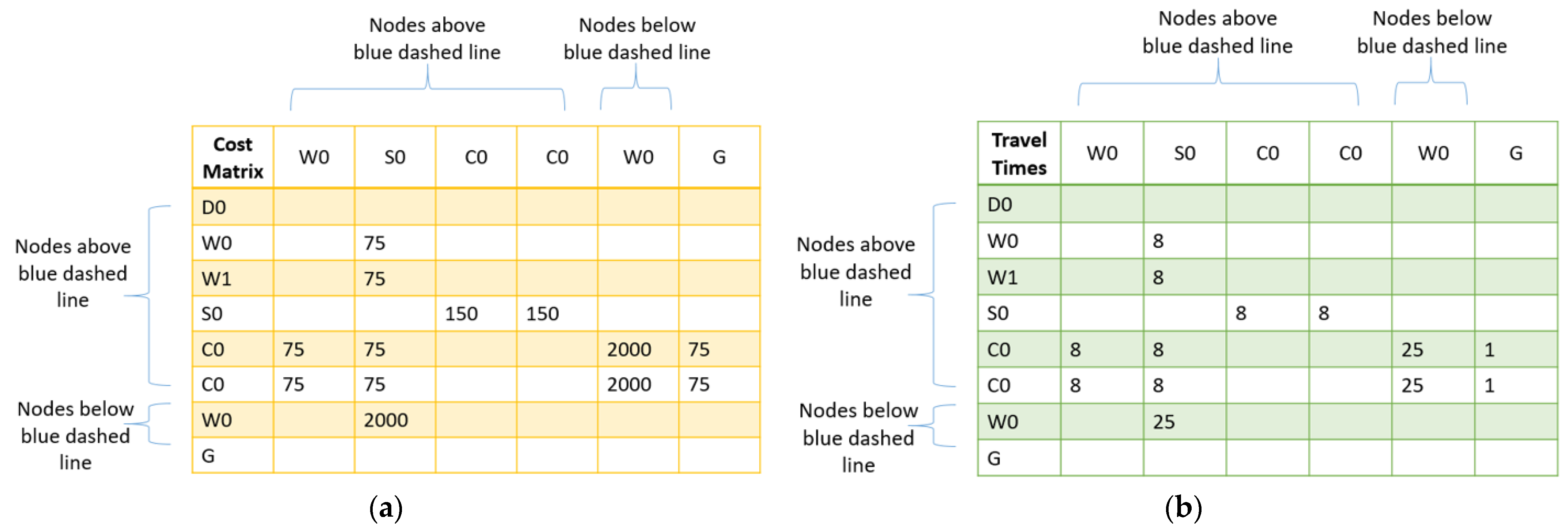
The cost matrix and travel time matrix corresponding to the first subproblem of the illustrative network depicted in Figure 1 are presented together under Figure 4 as Figure 4a and Figure 4b, respectively.

The network structure of the second subproblem of the small example in Figure 1 can be examined in Figure 5 below.

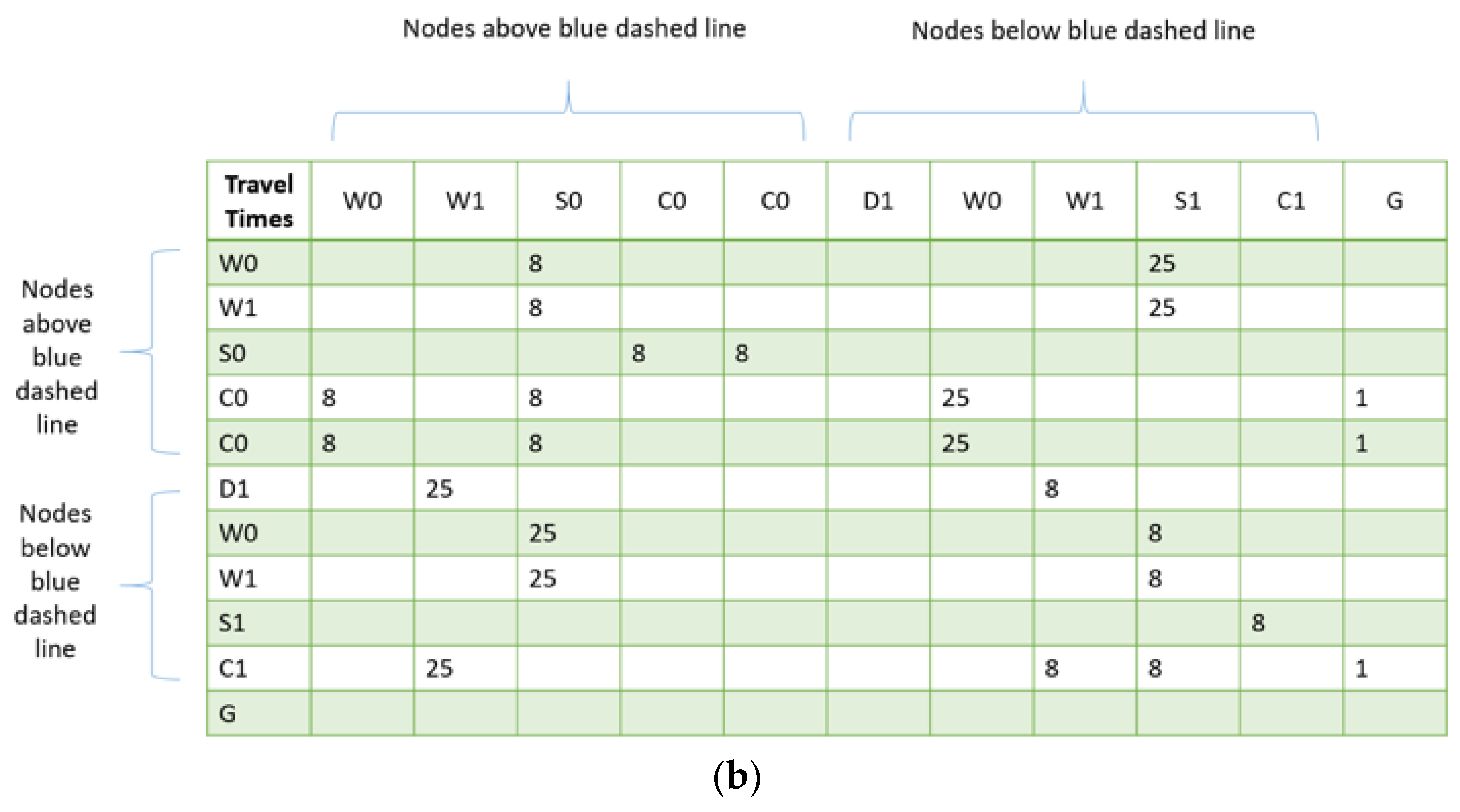
It should be emphasized that, although the blue trailer is technically capable of transporting both product types, no departures can be initiated from $D_0$ due to the absence of any vehicles equipped with a blue trailer at this location. Each subproblem is modeled as a network comprising a single departure node and a single garage node. For instance, if $D_0$ were to include rented vehicles equipped with a blue trailer, in addition to those present in the current numerical example, the total number of subproblems would increase to three. The cost matrix and travel time matrix corresponding to the second subproblem of the illustrative network depicted in Figure 1 are presented together in Figure 6a and Figure 6b, respectively.

ExampleExampleIt should be emphasized that the cost matrix associated with rented vehicles is comparatively more favorable than that of owned vehicles, as expressed in the problem definition part, primarily because expenses such as insurance, maintenance, and salaries are not accounted for in rented vehicles. In essence, the operational cost per kilometer for owned vehicles is generally higher than that for rented vehicles. In fact, the travel times of rented vehicles on a given arc may be either shorter or longer than those of owned vehicles. However, to maintain the clarity and simplicity of the illustrative example in Figure 1, the travel times for rented and owned vehicles are assumed to be identical. Consequently, the travel times for shared arcs are treated as the same across both the subproblem networks that are depicted in Figure 3 and Figure 5.

The blue dashed line depicted in Figure 1 serves as a crucial reference, highlighting the significant separation between the two vehicles in the example problem. This separation arises because any traversal across the line, from below to above or vice versa, incurs substantial costs and travel time. If truck driver scheduling constraints were not considered, then optimal path solutions would be expected to remain entirely either above or below the dashed line, respecting time windows constraints. At optimality, the first subproblem would produce the blue path illustrated in Figure 7.

At optimality, the second subproblem would yield the red path in Figure 8 below.

If the optimal routes previously identified in Figure 7 and Figure 8 also comply with the break–rest–drive constraints, they will continue to constitute the optimal solution. Conversely, if these constraints are not met, alternative routes, necessarily associated with a higher total cost, must be determined for optimality. Since the routes in Figure 7 and Figure 8 adhere to the relevant driver regulations, they are retained as the optimal paths, with the corresponding solutions presented in Figure 9 below.

As depicted in Figure 9, each numerical value represents a discrete time unit, with each unit corresponding to a duration of 30 min. Furthermore, the regulatory framework established by the United States Federal Motor Carrier Safety Administration, as explicitly outlined in Section 4, is applied in this context. For example, $t^{elapsed|R}$, $t^{elapsed|B}$, $t^{drive|R}$, $t^{rest}$, and $t^{break}$ become 28, 16, 22, 20, and 1 h, respectively, instead of 14, 8, 11, 10, and 0.5 h. While executing the scheduling of these optimal paths, waiting times may arise at the visited nodes. Consequently, the required rest periods must be extended, resulting in durations exceeding $t^{rest}$ or 20 time units, as illustrated in Figure 9. In contrast, the break periods can be maintained at their minimum duration, since no additional waiting occurs at the nodes visited after the break periods, as also depicted in Figure 9.

As illustrated in Figure 3, certain arcs have been deliberately omitted from the network. This modification arises from the operational constraint that the green trailer is incompatible with the transportation of first-type products. Consequently, it must be precluded from accessing any supply, washing, or customer nodes associated with this product category.

To summarize, Figure 1 represents only a small illustrative network of the specified FTL problem. In a large-scale version, the network would include a substantially greater number of departure nodes and a large fleet of both rented and owned vehicles that are located at these nodes connecting to various trailer types, as well as a greater number of washing centers, customer nodes, supply nodes, and product types compared to those shown in Figure 1.

4. Methodology

4.1. Construction Heuristic

Regarding the network structure of the problem, an insertion-based method inspired by Solomon [7] is involved. This method involves gradually adding nodes to a route in a feasible way until all contracted customers are served. It is important to note that non-contracted customers do not need to be satisfied as it is not required that they be visited. In order to create a route for a vehicle quickly, vehicles are allowed to travel from supply nodes to the garage node, washing nodes to the garage node, or departure nodes to the garage node with the employment of relevant arcs. Undoubtedly, during the CG iterations, these arcs are deleted. Routes/columns that have been found by the heuristic algorithm which include such arcs can also be avoided in CG iterations that introduce prohibitive costs (big M values) for them.

The pseudo-code of the construction heuristic can be examined in Algorithm 1.

Algorithm 1. Pseudo-Code of Construction Heuristic

Step 1: Select a vehicle which has not been assigned to a route. Step 2: Insert nodes in a feasible way based on forward labelling procedures in Table 3 and Table 4. Step 3: If the vehicle visits a contracted customer node, then do not allow vehicles to visit this node again. Step 4: If the vehicle reaches the garage node, then return to Step 1; otherwise, return to Step 2. Step 5: If all contracted customer nodes are not visited by vehicles, then delete all routes of vehicles generated so far and return to Step 1. Step 6: If all contracted customers are visited, then obtain initial routes/columns.

Due to long-haul transportation, rest–break policies should be embedded and path generation algorithms should respect these policies. In order to insert nodes by making suitable extensions and obtaining routes for each vehicle, label-updating processes in forward labeling with the equations provided in Table 3 and Table 4 are included. In short, the actions in Table 3 and Table 4 must be merged with the construction heuristic algorithm to deal with rest–break–drive constraints. Furthermore, the algorithm continues to allocate paths for vehicles until there are no contracted customers left, since each vehicle is conceived of as a route in the overall problem.

Table 3. Extension functions for forward labeling.

Labels/Functions	${\mathit{f}}_{\mathit{i}\mathit{j}}^{\mathit{s}\mathit{t}\mathit{a}\mathit{r}\mathit{t}}$	${\mathit{f}}_{\mathit{i}\mathit{j}}^{\mathit{d}\mathit{r}\mathit{i}\mathit{v}\mathit{e}}(∆)$	${\mathit{f}}_{\mathit{i}\mathit{j}}^{\mathit{b}\mathit{r}\mathit{e}\mathit{a}\mathit{k}}(∆)$	${\mathit{f}}_{\mathit{i}\mathit{j}}^{\mathit{r}\mathit{e}\mathit{s}\mathit{t}}(∆)$
$l^{cost}$	$l^{cost}+{\overline{c}}_{ij}$
$l^{time}$		$l^{time}+∆$	$l^{time}+∆$	$l^{time}+∆$
$l^{dist}$	$t_{ij}$	$l^{dist}-∆$
$l^{drive|R}$		$l^{drive|R}-∆$		0
$l^{elapsed|R}$		$l^{elapsed|R}+∆$	$l^{elapsed|R}+∆$	0
$l^{elapsed|B}$		$l^{elapsed|B}+∆$	0	0
$l^{latest|R}$				∞
$l^{latest|B}$		$min(l^{latest|B}, l^{latest|R}+t^{elapsed|R}-l^{elapsed|B}-∆)$	∞	∞

Table 3. Extension functions for forward labeling.

Labels/Functions	${\mathit{f}}_{\mathit{i}\mathit{j}}^{\mathit{s}\mathit{t}\mathit{a}\mathit{r}\mathit{t}}$	${\mathit{f}}_{\mathit{i}\mathit{j}}^{\mathit{d}\mathit{r}\mathit{i}\mathit{v}\mathit{e}}(∆)$	${\mathit{f}}_{\mathit{i}\mathit{j}}^{\mathit{b}\mathit{r}\mathit{e}\mathit{a}\mathit{k}}(∆)$	${\mathit{f}}_{\mathit{i}\mathit{j}}^{\mathit{r}\mathit{e}\mathit{s}\mathit{t}}(∆)$
$l^{cost}$	$l^{cost}+{\overline{c}}_{ij}$
$l^{time}$		$l^{time}+∆$	$l^{time}+∆$	$l^{time}+∆$
$l^{dist}$	$t_{ij}$	$l^{dist}-∆$
$l^{drive|R}$		$l^{drive|R}-∆$		0
$l^{elapsed|R}$		$l^{elapsed|R}+∆$	$l^{elapsed|R}+∆$	0
$l^{elapsed|B}$		$l^{elapsed|B}+∆$	0	0
$l^{latest|R}$				∞
$l^{latest|B}$		$min(l^{latest|B}, l^{latest|R}+t^{elapsed|R}-l^{elapsed|B}-∆)$	∞	∞

Table 4. Visit function for forward labeling.

Labels/Function	${\mathit{f}}_{\mathit{i}\mathit{j}}^{\mathit{v}\mathit{i}\mathit{s}\mathit{i}\mathit{t}}$
$l^{cost}$
$l^{time}$	$\max \left(a_j,l^{time}\right)+s_j$
$l^{dist}$
$l^{drive|R}$
$l^{elapsed|R}$	$\max \left(l^{elapsed|R}, a_j-l^{latest|R} \right)+s_j$
$l^{elapsed|B}$	$\max \left(l^{elapsed|B}, a_j-l^{latest|B} \right)+s_j$
$l^{latest|R}$	$\max \left(l^{latest|R}, b_j+s_j-l^{elapsed|R} \right)$
$l^{latest|B}$	$\max \left(l^{latest|B}, b_j+s_j-l^{elapsed|B} \right)$

Table 4. Visit function for forward labeling.

Labels/Function	${\mathit{f}}_{\mathit{i}\mathit{j}}^{\mathit{v}\mathit{i}\mathit{s}\mathit{i}\mathit{t}}$
$l^{cost}$
$l^{time}$	$\max \left(a_j,l^{time}\right)+s_j$
$l^{dist}$
$l^{drive|R}$
$l^{elapsed|R}$	$\max \left(l^{elapsed|R}, a_j-l^{latest|R} \right)+s_j$
$l^{elapsed|B}$	$\max \left(l^{elapsed|B}, a_j-l^{latest|B} \right)+s_j$
$l^{latest|R}$	$\max \left(l^{latest|R}, b_j+s_j-l^{elapsed|R} \right)$
$l^{latest|B}$	$\max \left(l^{latest|B}, b_j+s_j-l^{elapsed|B} \right)$

Recalling from the CG model above, non-contracted customers’ requests do not have to be satisfied. Hence, excluding non-contracted customers helps reduce the size of the search in the heuristic algorithm and makes the network lighter. This is because their exclusion decreases the total number of nodes and arcs connected to them. It is important to remember that the computational complexity of path generation algorithms is influenced by the total number of arcs and nodes. Therefore, in a simplified network, constructing or extending routes in a feasible manner requires less complexity.

4.2. Column Generation Algorithm

The literature suggests that column generation methods are highly effective in solving partitioning problems in an exact way. One can refer to the studies of Savelsbergh [34] for the generalized assignment problem or de Carvalho et al. [35] for the cutting stock problem to gain insights into the types of problem concepts that can be partitioned. Undoubtedly, the vehicle routing problem (VRP) is one of the toughest partitioning problems when aiming for optimality with an exact algorithm. In the realm of VRPs, CG methods have demonstrated notable benefits (Desrosiers et al. [31]) in managing extensive VRP variants when compared to other approaches like mixed-integer programming or the branch and cut/bound method, owing to their outstanding efficiency. For example, mixed-integer programming handles small-scale instances because it reaches exponential complexity in a short period of time for large scale ones, while the branch and cut technique can deal with middle-scale instances with some clever cuts but reaches exponential complexity again in large-scale ones. However, CG methods are superior to them due to their pseudo-polynomial complexity even in large-scale instances thanks to the structure of pricing problems in CG methods. One can also enrich their CG model with different types of cuts and branching methods, which encourages a considerable number of studies to be centered around BPC algorithms. Nevertheless, our algorithm does not include branching as it already achieves a minimal optimality gap at the root node. In essence, it can be said that the proposed algorithm can be classified as a BPC algorithm. Undoubtedly, as a VRP variant becomes increasingly complex, the labeling procedures, which are crucial to the column generation method, become significantly more challenging to derive. Therefore, if labels cannot be defined in accordance with the feasible solutions of the relevant VRP variant, the column generation approach cannot be employed.

The label-setting algorithm used in CG methods to generate columns/routes is known to have pseudo-polynomial time complexity by constituting a bottleneck for the entire process, as shown in Figure 10, making it a pseudo-polynomial time algorithm overall. Complexity analysis can be performed with the inclusion of Dial et al. [36] for the label-correcting algorithm and Feillet, Dominique et al. [37] for the routes/columns’ constraints with respect to resources, each of which corresponds to a dimension in the label-setting algorithm.

It must also be emphasized that the CG method has two serial algorithms within itself, one of which is based on the solution of the RMP, while the other is based on finding promising columns/routes. Whereas interior point methods, which are polynomial time algorithms, can solve the RMP, the nested label-setting algorithm is deployed to find a suitable column/route with pseudo-polynomial time complexity. Therefore, the nested label-setting algorithm outweighs the CG method with regard to complexity analysis.

In the realm of exact algorithms, acceleration techniques called bi-directional search (Righini et al. [11]), heuristic pricing algorithm (Desaulniers et al. [10]), and ng-route relaxation (Baldacci et al. [12]) have demonstrated superior performance and are commonly utilized in comparison to others in the literature in combination with CG processes. Therefore, our approach incorporates the most effective exact algorithm and acceleration concepts from the VRP literature following the implementation of a construction heuristic. Additionally, it is crucial to recognize that CG methods and their acceleration concepts are specific to the problem at hand. Therefore, one must adapt them accordingly when faced with a novel problem, as we did in our study.

The RMP, which is the integer-relaxed version of the CG model, is indispensable as its optimal value serves as a lower bound generated by CG processes while an upper bound can be derived from the columns/routes created up to that point. The pricing problem that belongs to our specified FTL network must always be addressed for specific subproblems. In terms of the CG model, $\sum _{o\in O}\sum _{i\in I_o}\sum _{j\in J}1$ represents the number of all subproblems. Each of them depends on a given trailer $o\in O,$ a departure node $i\in I_o$ for that trailer, and a vehicle type $j\in J$ connected with that trailer. Additionally, each subproblem is associated with its own network, allowing for the departure of a specific vehicle category that is connected to a corresponding trailer from the designated point. Under a certain $o\in O,$ $i\in I_o$, and $j\in J$ for the relevant subproblem, a pricing problem can be established as follows.

$$\underset{p\in P}{\min } {\overline{c}}_{oijp}$$

subject to the following:

• Vehicles must obey time windows.
• Vehicles can visit each customer point no more than once.
• Vehicle drivers must obey rest–break policies imposed by driving regulations.

In the pricing problem mentioned earlier, $P$ represents the set of all possible routes in the specific subproblem where each customer node is visited no more than once, time window constraints are not violated, and truck driver scheduling constraints are not breached.

$$\begin{array}{cc}{\overline{c}}_{oijp}=c_{oijp}\hfill & - {\displaystyle \sum _{q\in C}}{a}_{oijpq}\ast {\alpha }_q-{\displaystyle \sum _{q^{\prime }\in C^{\prime }}}{a}_{oijp{q}^{\prime }}\ast {\alpha }_{q^{\prime }}\hfill \\ & -{\displaystyle \sum _{U\in P\left(C\right)}}{\displaystyle \sum _{\left(m,n\right) \in A^{-}\left(U\right)}}{b}_{oijpmn}\ast {\lambda }_U\hfill \\ & - {\displaystyle \sum _{\left(m^{\prime },n^{\prime }\right) \in A^{\ast }\left(CW\right)}}{\displaystyle \sum _{\left(m,n\right) \in A^{\ast }\left(m^{\prime },n^{\prime }\right)}}{b}_{oijpmn}\ast {p1}_{m^{\prime }{n}^{\prime }}\hfill \\ & - {\displaystyle \sum _{\left(m^{\prime },n^{\prime }\right) \in A^{\ast }\left(SC\right)}}{\displaystyle \sum _{\left(m,n\right) \in A^{\ast }\left(m^{\prime },n^{\prime }\right)}}{b}_{oijpmn}\ast {p2}_{m^{\prime }{n}^{\prime }}\hfill \end{array}$$

(10)

In Equation (10), $c_{oijp}$ is the cost of the route, while ${\alpha }_q$, ${\alpha }_{q^{\prime }}$, ${\lambda }_U$, ${p1}_{m^{\prime }{n}^{\prime }}$, and ${p2}_{m^{\prime }{n}^{\prime }}$ are the dual variables that correspond to the number of visits to contracted customers (Constraint (2)), the number of visits to non-contracted customers (Constraint (3)), 2-path inequalities (Constraint (5)), and arc flow constraints (Constraints (6) and (7)), respectively. In terms of the subproblem under consideration, $\beta$ is the dual variable of the relevant Constraint (4), which has $H_{oij }$ on the right-hand side of the inequality. Lastly, ${\overline{c}}_{oijp}$ is the reduced cost associated with the route.

4.2.1. Nested Label-Setting Algorithm

This algorithm must be implemented for each subproblem in the CG model. Actually, each subproblem has its own network, and vehicles that can traverse the arcs of that network have a limit of $H_{oij }$, as in (4). Hence, in order to improve the RMP, one should examine all the subproblems’ networks to determine favorable columns/routes. The lack of a column that cannot improve RMP implies the optimality of the RMP, and the optimal value is a lower bound for the model.

The works of Tilk [15] and Goel and Irnich [16] were the first ones to address the VRP with consideration of truck driver scheduling using BPC algorithms. Tilk and Goel [17] expanded the previous studies, including effective acceleration concepts and regulations from different countries. Both works introduced efficient label variables for a nested label-setting algorithm to comply with scheduling constraints and devised dominance rules to expedite the solution process. Because scheduling constraints are crucial in our work, we adopted and implemented their methods with some modifications. Additionally, we paid attention to the work of Feillet et al. [37] and Righini et al. [11,38], who devised efficient labeling techniques called forward and backward labeling for addressing basic shortest path problems with resource constraints. Their studies helped us acquire routes/columns for the column generation process in our work while searching for the lower bound of our problem. Thus, a modified version of their methodologies was also incorporated accordingly.

According to the rules (Hours of Service Regulations, enforced by the United States Federal Motor Carrier Safety Administration), a driver in the U.S. should take breaks, rest, or drive on long-distance routes. In accordance with the parameters stipulated by United States regulatory standards, the following notations are adopted: $t^{drive|R}$ represents the maximum allowable driving time between two successive rest periods; $t^{break}$ denotes the minimum permissible duration of a break; $t^{rest}$ indicates the minimum required length of a rest period; $t^{elapsed|B}$ corresponds to the maximum time permitted after the conclusion of a break period before driving may resume; and $t^{elapsed|R}$ designates the maximum time allowed after the completion of a rest period before driving may commence. Therefore, it can be put into words that a driver should not exceed $t^{elapsed|B}$ and $t^{elapsed|R}$ while driving their truck. Otherwise, this may lead to huge fines imposed by traffic control crews.

Consistent with the aforementioned United States regulations, the forward labels employed in the nested label-setting algorithm, elements that are pivotal to the forward labeling process, must encapsulate the following components: the reduced cost associated with the forward path ($l^{cost}$); the total elapsed time since the initiation of the forward path ($l^{time}$); the remaining driving time required to reach the next customer along the forward path ($l^{dist}$); the cumulative driving time accrued since the most recent rest period ($l^{drive|R}$); the elapsed time measured from the conclusion of the preceding rest period ($l^{elapsed|R}$); the elapsed time measured from the conclusion of the preceding break period ($l^{elapsed|B}$); the latest permissible time to which the prior rest period can be extended without breaching scheduling constraints ($l^{latest|R}$); and the latest permissible time to which the prior break period can be extended without violating scheduling requirements ($l^{latest|B}$). Thus, it can be expressed that $l^{elapsed|R}$ and $l^{elapsed|B}$ aim to maintain the energy of a driver on their route, while $l^{latest|R}$ and $l^{latest|B}$ support the elimination of redundant waiting times for the driver during node visits.

During the forward labeling iterations, each forward label has a forward path, label variables, as defined above, and visited customer nodes’ spaces. That is why each forward label is defined as $L_i(v_i,{ S}_i,T_i)$ in this study. A forward path becomes $PF=(v_0,v_1\dots ,v_i)$, where $v_i$ is the $i^{th}$ node/vertex in the network. Thus, this implies that, according to $PF$, vehicles should depart at $v_0$ (a departure node in the network), then visit $v_1, v_{2,} v_{3 } \mathrm{a}\mathrm{n}\mathrm{d} v_4$ consecutively until $v_i$. ${ S}_i$ keeps the set of visited customer nodes, while $T_i=(l^{cost},l^{time},l^{dist},l^{drive|R},l^{elapsed|R},l^{elapsed|B},l^{latest|R},l^{latest|B})$. It must be noted that washing nodes and supply nodes can be visited multiple times by a vehicle, while contracted and non-contracted customers can at most be visited once. That is why ${ S}_i$ is included to track the number of visits to customer points/nodes. Furthermore, for the initialization of a forward label and recursive extension of this label, $L_0(v_0,\varnothing ,T_0)$ is taken into consideration, setting $T_0=(\mathrm{0,0},\mathrm{0,0},\mathrm{0,0},\infty ,\infty )$.

To provide labels with an extension, Table 3 and Table 4 are utilized if there is a feasible arc from the $i^{th}$ node to the $j^{th}$ node. However, although an arc exists between these nodes, one must additionally ensure that $j$∉${NG}_i$ or $j\notin S_i$ and $l^{time}+ t_{ij}\le b_j$. ${NG}_i$ is the predefined neighborhood set associated with node $i$, whereas $t_{ij}$ is the driving time required to travel from the $i^{th}$ node to the $j^{th}$ node, and $b_j$ is the upper bound of selected time windows of the $j^{th}$ node. Indeed, these situations render the utilization of $f_{ij}^{start}$ operationally viable. Given the presence of multiple time windows, $[a_j,b_j]$ denotes one of the admissible service intervals for the $j^{th}$ node. $s_j$ is the service duration at that node. After the label has been extended, $S_j= S_i \bigcup \left\{j\right\}$ is derived for $L_j(v_j,{ S}_j,T_j)$, whereas $j\in (C\cup C^{\prime })$.

Blank spaces in two tables above imply that there will be no change for the relevant forward label variable during the relevant extension function. According to Table 3, $∆$ denotes the duration associated with driving, rests, and breaks corresponding to $f_{ij}^{drive}(∆)$, $f_{ij}^{break}(∆)$, and $f_{ij}^{rest}(∆)$, respectively. Undoubtedly, these functions cannot be employed at every point in the timeline; therefore, feasibility conditions take place to benefit from them, as shown in

Table 5. Feasibility conditions of extension functions in forward labeling.

Functions	Feasibility Conditions
$f_{ij}^{start}$	$j$∉${NG}_i$ or $j\notin S_i$ and $l^{time}+ t_{ij}\le b_j$
$f_{ij}^{drive}(∆)$	${0<∆ \le ∆}_l=\mathrm{m}\mathrm{i}\mathrm{n}(l^{dist},t^{drive|R}-l^{drive|R},t^{elapsed|R}-l^{elapsed|R}, t^{elapsed|B}-l^{elapsed|B})$
$f_{ij}^{break}(∆)$	${0\ge ∆}_l =\mathrm{m}\mathrm{i}\mathrm{n}(l^{dist},t^{drive|R}-l^{drive|R},t^{elapsed|R}-l^{elapsed|R}, t^{elapsed|B}-l^{elapsed|B})$ and $∆ \ge t^{break}$
$f_{ij}^{rest}(∆)$	${0\ge ∆}_l =\mathrm{m}\mathrm{i}\mathrm{n}(l^{dist},t^{drive|R}-l^{drive|R},t^{elapsed|R}-l^{elapsed|R}, t^{elapsed|B}-l^{elapsed|B})$ and $∆ \ge t^{rest}$
$f_{ij}^{visit}$	$l^{time}\le b_j$ and $l^{dist}=0$

. Nevertheless, if $c_{ij}$ is transformed with the dual variables, as shown in Equation (10), then ${\overline{c}}_{ij}$ is acquired.

With respect to Table 5, it is emphasized that ${∆}_l$ indicates how many more time units a driver can drive for at a given moment without breaching the regulations. Therefore, that is why the drive function, called $f_{ij}^{drive}(∆)$, includes the structure of ${∆}_l$, and $∆$ cannot exceed the value of ${∆}_l$.

The dominance rules, which aim to prevent an excessive increase in the total number of labels, were created by Tilk [15] as well as Goel and Irnich [16] and were employed in our study as follows: Driving function is imposed when ${∆}_{l }>0$ and $l^{dist}>0$. This is because this circumstance prevents redundant break and rest periods while driving is possible. If a rest or break is enforced due to ${∆}_l =0$ (driving is impossible), then these periods are taken as $t^{rest}$ and $t^{break}$. This is because these periods are stretched when needed due to the extension function called $f_{ij}^{visit}$. Subsequently, consecutive occurrences of two rest periods, two break periods, a rest period immediately following a break, or a break immediately following a rest period are prohibited, as such sequences represent operationally meaningless combinations. Nevertheless, if there is a situation such as ${{ S}_i}^1\subseteq {{ S}_i}^2$, ${l^1}^{cost}\le {l^2}^{cost}$, ${l^1}^{time}\le {l^2}^{time}$, ${l^1}^{dist}\le {l^2}^{dist}$, ${l^1}^{drive|R}\le {l^2}^{drive|R}$, ${l^1}^{elapsed|R}\le {l^2}^{elapsed|R}$, ${l^1}^{elapsed|B}\le {l^2}^{elapsed|B}$, ${l^1}^{latest|R}\ge {l^2}^{latest|R}$, or ${l^1}^{latest|B}\ge {l^2}^{latest|B}$, then the forward label regarding the $i^{th}$ node, called ${L_i^1(v}_i,{{ S}_i}^1,{T_i}^1)$, dominates and has the potential to outperform the forward label regarding the $i^{th}$ node called $L_i^2(v_i,{{ S}_i}^2,{T_i}^2)$. It implies that whenever $L_i^2(v_i,{{ S}_i}^2,{T_i}^2)$ is feasibly extended with any extension function, ${L_i^1(v}_i,{{ S}_i}^1,{T_i}^1)$ can be likewise extended. After the extension, the label variables of ${L_i^1(v}_i,{{ S}_i}^1,{T_i}^1)$ continue to outperform the label variables of $L_i^2(v_i,{{ S}_i}^2,{T_i}^2)$.

By virtue of symmetry, an analogous procedure to the aforementioned forward label approach can be implemented for backward labels, wherein the backward path is represented as $PB=(v_0^b,v_1^b\dots ,v_i^b)$. $v_0^b$ is the terminal node, while $v_i^b$ has the same concept as $v_i$. When employing a large positive number, M, the time window $[a_i,b_i]$ for each node $v_i$ changes. As an example, $\left[a_i^b,b_i^b\right]= [{M-b}_i-s_i ,{ M-a}_i- s_i]$ with regard to backward labeling. It should be noted that, within the forward labeling framework, the time window boundaries represent the earliest and latest feasible starting times for processing at the corresponding node on timeline. In contrast, under the backward labeling approach, these boundaries denote the earliest and latest permissible departure times on the timeline from the respective node. While forward and backward labels share numerous structural similarities, subtle yet significant distinctions exist in their respective label-updating procedures.

A backward label associated with the previously defined backward path $PB$ from above can be represented as ${L_i}^b({v_i}^b,{{ S}_i}^b,{T_i}^b)$. ${T_i}^b=({l^{cost}}_b,{l^{time}}_b,{l^{dist}}_b,{l^{drive|R}}_b,{l^{elapsed|R}}_b,{l^{elapsed|B}}_b,{l^{latest|R}}_b,{l^{latest|B}}_b)$, and ${{ S}_i}^b$ has the same concept as $S_i$. Thus, the backward label is initialized as ${L_o}^b({v_0}^b,\varnothing ,{T_0}^b)$, where ${T_0}^b=(\mathrm{0,0},\mathrm{0,0},\mathrm{0,0},\infty ,\infty )$.

In the context of backward labeling, ${f_{ij}^{start}}^b$, ${f_{ij}^{drive}(∆)}^b$, ${f_{ij}^{break}(∆)}^b$, ${f_{ij}^{rest}\left(∆\right)}^b$, and ${f_{ij}^{visit}}^b$ correspond to $f_{ij}^{start}$, $f_{ij}^{drive}(∆)$, $f_{ij}^{break}(∆)$, $f_{ij}^{rest}\left(∆\right)$, and $f_{ij}^{visit}$, respectively. While forward labeling involves traversing an arc from the $i^{th}$ node to the $j^{th}$ node, backward labeling requires reverse movement along this arc. Specifically, for example, ${f_{ij}^{start}}^b$ starts the reverse arc movement towards the $j^{th}$ node from the $i^{th}$ node. The feasibility conditions and updating procedures for ${f_{ij}^{start}}^b$, ${f_{ij}^{drive}(∆)}^b$, ${f_{ij}^{break}(∆)}^b$, and ${f_{ij}^{rest}\left(∆\right)}^b$ are totally analogous to their counterparts in forward labeling. However, ${f_{ij}^{visit}}^b$ entails two extra conditions to ensure feasible extension, which are ${f_{ij}^{visit}}^b\left({l^{elapsed|R}}_b\right)\le t^{elapsed|R}$ and ${f_{ij}^{visit}}^b\left({l^{elapsed|B}}_b\right)\le t^{elapsed|B}$. Nevertheless, ${f_{ij}^{visit}}^b$ updates ${l^{cost}}_b,{ l^{time}}_b, { l^{dist}}_b, {l^{drive|R}}_b$ in the same manner as in the forward labeling procedures. In contrast, ${l^{elapsed|R}}_b, { l^{elapsed|B}}_b,{{ l}^{latest|R}}_b,{ l^{latest|B}}_b$ are altered using a different strategy. These strategies can be observed in

Table 6. Visiting function during backward labeling.

Labels/Function	${{\mathit{f}}_{\mathit{i}\mathit{j}}^{\mathit{v}\mathit{i}\mathit{s}\mathit{i}\mathit{t}}}^{\mathit{b}}$
${l^{elapsed|R}}_b$	$\left\{\begin{array}{c}0,\\ \max \left({l^{elapsed|R}}_b, {a_j}^b-{l^{latest|R}}_b \right)+s_{j,}\end{array}{\displaystyle \genfrac{}{}{0pt}{}{\mathrm{I}\mathrm{f} {l^{elapsed|R}}_b=0}{\mathrm{o}\mathrm{t}\mathrm{h}\mathrm{e}\mathrm{r}\mathrm{w}\mathrm{i}\mathrm{s}\mathrm{e}}}\right.$
${l^{elapsed|B}}_b$	$\left\{\begin{array}{c}0,\\ \max \left({l^{elapsed|B}}_b, {a_j}^b-{l^{latest|B}}_b \right)+s_j,\end{array}{\displaystyle \genfrac{}{}{0pt}{}{\mathrm{I}\mathrm{f} {l^{elapsed|B}}_b=0}{\mathrm{o}\mathrm{t}\mathrm{h}\mathrm{e}\mathrm{r}\mathrm{w}\mathrm{i}\mathrm{s}\mathrm{e}}}\right.$
${l^{latest|R}}_b$	$\left\{\begin{array}{c}\infty ,\\ \max \left({l^{latest|R}}_b, {b_j}^b+s_j-{l^{elapsed|R}}_b \right),\end{array}{\displaystyle \genfrac{}{}{0pt}{}{ \mathrm{I}\mathrm{f} {l^{elapsed|R}}_b=0}{\mathrm{o}\mathrm{t}\mathrm{h}\mathrm{e}\mathrm{r}\mathrm{w}\mathrm{i}\mathrm{s}\mathrm{e}}}\right.$
${l^{latest|B}}_b$	$\left\{\begin{array}{c}\infty ,\\ \max \left({l^{latest|B}}_b, b_j+s_j-{l^{elapsed|B}}_b \right),\end{array}{\displaystyle \genfrac{}{}{0pt}{}{\mathrm{I}\mathrm{f} {l^{elapsed|B}}_b=0}{\mathrm{o}\mathrm{t}\mathrm{h}\mathrm{e}\mathrm{r}\mathrm{w}\mathrm{i}\mathrm{s}\mathrm{e}}}\right.$

.

Due to the structure of extension functions with respect to backward labeling, the same dominance rules in forward labeling can again be deployed to discard dominated backward labels.

It must be noted that washing nodes behave a bit differently compared to other nodes. This is because the processing time of a washing node, which is related to its product type, can vary according to the supply node that is about to be visited next. Therefore, at a washing node, the processing time is always taken as the minimum duration in the row of the corresponding product type at that node in the washing matrix. Hence, during the feasibility check of the extension towards a supply node, recalling that one can move from washing nodes to supply nodes only in forward labeling, extra processing time can be added and decisions can be made without loss of generality. Furthermore, when a feasible extension occurs from the current washing node to a supply node in forward labeling, extra processing time is added, and labels are updated without loss of generality at the beginning of travel. On the other hand, in backward labeling, one can only travel from supply nodes to washing nodes using reverse arcs. Therefore, when traveling to washing nodes from supply nodes, the amount of washing time at the end of the visit function is apparent.

4.2.2. Acceleration Techniques

Because of the fact that the acceleration techniques of the column generation method are frame- and heavily problem-dependent, one is required to employ distinct implementations, and completely different labels and labeling procedures should be taken into account with regard to distinct problem concepts. While the VRP literature commonly relies on column generation methods to achieve precise solutions for large-scale instances, there is also significant interest in accelerating these methods. For instance, the label-setting algorithm often generates a large number of labels, which can create computational challenges during the solution process. Moreover, prioritizing subproblems becomes crucial when dealing with a high volume of them, as exhaustively searching for potential columns within each subproblem and identifying unpromising candidates can significantly slow down the solution process.

Due to the fact that CG methods necessitate the frequent use of a label-setting algorithm to generate columns for the RMP and this algorithm creates a bottleneck in Figure 10, accelerating the column generation process significantly reduces the overall complexity of the entire procedure. To expedite our RMP, we incorporated four commonly used acceleration concepts in VRP-oriented BPC algorithms.

Heuristic Pricing Algorithm

In the label-setting algorithm, determining the column with the most advantageous reduced cost may require a substantial amount of computational power because of the need to assess a significant number of labels (Desaulniers et al. [10]).

To alleviate the computational burden, we used a heuristic concept where we selected the first column with an advantageous reduced cost in a subproblem instead of deeply investigating the best. If one cannot find any promising column in a subproblem, then one should move on to consider others consecutively. If subproblems do not provide a favorable column, it means that the RMP has already attained optimality. This acceleration technique, as shown by Desaulniers et al. [10], efficiently identifies a favorable column in a subproblem, which is then added to the RMP to calculate new dual variables and continue the CG iterations. One should also dive into the details of Desaulniers et al. [10] to grasp the concept of their valuable study and to observe the big improvement it has contributed. It must be noted that, although this acceleration technique has a heuristic approach, it is capable of examining all columns/routes in the design by Desaulniers et al. [10] (see Algorithm 2).

Algorithm 2. Pseudo-Code of Heuristic Pricing Algorithm

Step 1: Get the dual variables using the current RMP. Step 2: Merge these dual variables with the arc costs of the relevant subproblem. Step 3: Initialize a label based on the relevant departure node. Step 4: Put the initial label into a label set. Step 5: Expand the label set towards the terminal/garage node using relevant nested label-setting procedures. Step 6: If the last node of the path of a label is the terminal/garage node and it is capable of improving the RMP, then use this path and add as a column to RMP, solve RMP and return to Step 1.

Heuristic Subproblem Selection

Due to the fact that there is a huge number of subproblems, as is mentioned above, a tactic should be adopted accordingly. It is indeed plausible to assess all subproblems in an established order until a favorable column is found. However, this method can dramatically prolong the computational time needed to identify such a column. For instance, as the RMP progresses through iterations, certain subproblems may not yield columns that enhance the RMP. This can lead to a substantial increase in computational time for the entire solution process. To tackle this challenge, this method prioritizes the most recent subproblem that has provided a favorable column for the RMP, instead of assessing all of them.

It is worth highlighting that this method is an enhancement of the first acceleration method proposed by Desaulniers et al. [10]. While the heuristic pricing algorithm determines the initial favorable column when only one subproblem is present in the overall problem, this method concentrates on determining the first advantageous path/column among multiple subproblems. Therefore, it is crucial to dive into the details of the heuristic pricing algorithm to deeply or at least intuitively understand the concept of the heuristic’s subproblem selection. Thus, instead of exhaustively searching for the best column/route among all those derived from all subproblems, this acceleration technique focuses on a prioritized subproblem and attempts to obtain the first encountered promising column/route (see Algorithm 3).

Algorithm 3. Pseudo-Code of Heuristic Subproblem Selection

Step 1: Select the subproblem that has generated the previous column improving the RMP. Step 2: Get the dual variables using the current RMP. Step 3: Merge these dual variables with the arc costs of the relevant subproblem. Step 4: Initialize a label based on the relevant departure node. Step 5: Put the initial label into a label set. Step 6: Expand the label set towards the terminal/garage node using relevant nested label-setting procedures. Step 7: If a column can be found to improve the RMP, then add this column to RMP, solve RMP and return to Step 1. Step 8: If no column can be found to improve the RMP, then select one of the remaining subproblems and return to Step 2.

NG-Route Relaxation

Baldacci et al. [12] presented the ng-route relaxation technique for VRP(s) with time windows. The label-setting algorithm includes elementary paths to define the optimal paths’ structures, but the relaxation concept also incorporates non-elementary paths to expedite the termination of the RMP. During the label-setting algorithm, checking whether the path has remained elementary (single visit for each customer node) increases complexity. Therefore, this relaxation technique enhances convergence speed, despite causing a decline in the RMP’s lower bound according to Baldacci et al. [12]. However, their research indicates that the relaxation’s impact on the RMP optimality is not substantial. Therefore, one should dive into the details of their good work in order to visualize the concept and to observe the critical improvement they made. In their approach, an ng-set was assigned to each node with an established size, containing neighboring nodes as its elements.

Embracing this acceleration method, we let favorable routes encompass non-elementary routes, which involve cycles, to a limited extent by exploiting this method. Our problem is unique compared to typical vehicle routing problems because it involves extra node categories (washing and supply nodes), as opposed to customer nodes, departure nodes, and garage nodes. In typical vehicle routing problems, the nodes, except for the departure and terminal nodes, are always customer nodes, and they are always adjacent to at least one customer node. However, in our FTL network, customer nodes are not adjacent to another customer node. Instead, with respect to the forward arc structure, the neighborhood of supply nodes can be customer nodes, and with regard to the reverse arc structure, the neighborhood of washing and supply nodes can be customer nodes. Due to the fact that all ng-sets contain customer nodes according to Baldacci et al. [12], ng-sets during the forward labeling process are established with a focus on supply nodes, whereas ng-sets during the backward labeling process are established with a focus on both supply and washing nodes (see Algorithm 4).

Algorithm 4. Pseudo-Code of NG-Route Relaxation

Step 1: Execute the nested label-setting algorithm with the current dual variables merging these variables with arc costs of the relevant subproblem. Step 2: While deriving forward paths, include cycles as long as the NG-sets that have been created for forward labeling allow. Step 3: While deriving backward paths, include cycles as long as the NG-sets that have been created for backward labeling allow. Step 4: If a column is decided to be added to RMP after merging a forward and backward path, solve RMP and return to Step 1.

Bi-Directional Search

According to Righini and Salani [11], bi-directional search involves backward paths as well as forward paths. Forward paths should be extended with reference to a departure node whereas backward paths should be extended with reference to a terminal node. Under a given network that belongs to a chosen subproblem during CG iterations, forward labeling involves identifying suitable forward paths involving extension functions in Table 3 and Table 4 as we move towards the terminal node. On the other hand, backward labeling focuses on identifying feasible backward paths using extension functions from both Table 3 and Table 6 as we proceed to the departure node. Righini and Salani [11] showed that their concept was much more computationally efficient than mono-directional search. However, one should also dive into the details of the good work of Feillet, Dominique et al. [37] to comprehend mono-directional search, and then focus on Righini and Salani [11] to be able to observe their crucial improvement. This is because bi-directional search utilizes both the departure node and terminal node in creating routes through simultaneous forward and backward labeling procedures. The bi-directional approach considers two-dimensional perspectives in route creation, unlike the one-dimensional perspective of the mono-directional approach. During the generation of promising columns/routes, the bi-directional algorithm is capable of exploring more promising paths in a given time, simultaneously growing partial paths from the departure node and garage/terminal node as opposed to the mono-directional algorithm. In addition, to improve effectiveness more, Righini and Salani [11] introduced a resource-based bounding procedure during the concatenation of forward and backward paths. In this study, resource-based bounding procedure was embraced and $l^{time}$ was chosen to be a vital resource of paths. Thus, our forward paths in this work were restricted by $l^{time}\le {\displaystyle \frac{M}{2}}+s_j$ for $L_i(v_i,{ S}_i,T_i$), where $T_i=(l^{cost},l^{time},l^{dist},l^{drive|R},l^{elapsed|R},l^{elapsed|B},l^{latest|R},l^{latest|B})$ and $M$ is sufficiently a large number. The same bounding concept was applied to backward label extensions as well. Therefore, all paths that the mono-directional approach would encompass could be guaranteed. After both forward and backward labels were obtained, concatenation of these was performed to obtain a promising column/route for the column generation algorithm. Assuming $L_i(v_i,{ S}_i,T_i)$ and ${L_i}^b({v_i}^b,{{ S}_i}^b,{T_i}^b)$, which are the forward label and backward labels for the $i^{th}$ node, respectively, concatenation rules should be taken into account as follows:

$$\left|{ S}_i\cap {{ S}_i}^b\right|=1$$

(11)

$$l^{time}-s_i\le M-{l^{time}}_b$$

(12)

$$l^{drive|R}+{l^{drive|R}}_b\le t^{drive|R}$$

(13)

$$l^{latest|R}+t^{elapsed|R}\ge M-{l^{latest|R}}_b$$

(14)

$$l^{latest|B}+t^{elapsed|B}\ge M-{l^{latest|B}}_b$$

(15)

$$l^{elapsed|R}+{l^{elapsed|R}}_b-s_i\le t^{elapsed|R} \mathrm{or} l^{elapsed|R}\le s_i\mathrm{or} {l^{elapsed|R}}_b\le s_i$$

(16)

$$l^{elapsed|B}+{l^{elapsed|B}}_b-s_i\le t^{elapsed|B} \mathrm{or} l^{elapsed|B}\le s_i\mathrm{or} {l^{elapsed|B}}_b\le s_i$$

(17)

With respect to the concatenation rules, Equation (11) ensures the elementarity of the concatenated path in relation to customer nodes, while Inequality (12) guarantees the feasibility of arrival times at the node where the forward and backward paths are merged. Inequality (13) enforces the maximum allowable driving time between two successive rest periods along the merged path. Inequalities (14) and (16) ensure compliance with the maximum time permitted after the completion of a rest period before driving may resume on the concatenated path. Similarly, Inequalities (15) and (17) ensure adherence to the maximum time allowed after the conclusion of a break period before driving may recommence on the concatenated path (see Algorithm 5 and Algorithm 6).

Algorithm 5. Pseudo-Code of Bi-Directional Search

Step 1: Initialize a forward label based on the relevant departure node. Step 2: Put the initial forward label into a forward label set. Step 3: Expand forward labels in the forward label set towards terminal/garage node as long as $l^{time}\le {\displaystyle \frac{M}{2}}+s_j$ using nested label-setting Procedures. Step 4: Initialize a backward label based on the relevant terminal/garage node. Step 5: Put the initial backward label into a backward label set. Step 6: Expand backward labels in the backward label set towards the relevant departure node as long as ${l^{time}}_b\le {\displaystyle \frac{M}{2}}+s_j$ using nested label-setting Procedures. Step 7: Try to concatenate all forward and backward paths regarding forward and backward labels, respectively, to find the column that can improve the RMP best. Step 8: If such a column is found, then add it to RMP, solve RMP, return to Step 1.

Algorithm 6. Pseudo-Code of Concatenation

Step 1: Execute the bi-directional search. Step 2: Select a forward label and obtain the relevant forward path of it. Step 3: Select a backward label obtain the relevant backward path of it. Step 4: Try to combine these paths according to the conditions (11)–(17). Step 5: If conditions cannot be satisfied, then return to Step 3. Step 6: If there is no backward label left while conditions are not satisfied, return to Step 2. Step 7: If conditions are met, then create a new path/column merging these paths and keep.

5. Computational Study

5.1. Creation of Instances

Our problem structure has no benchmark sets in the literature, therefore instance sets were artificially created, benefiting from the actions of a Turkish logistics company that has a large fleet size (approximately 600 vehicles) and a strong background in liquid transportation. We set up relevant intervals for arc expenses, travel durations, processing times, washing expenses, and revenues regarding non-contracted clients. Random values were created within these parameters with respect to a uniform distribution to reflect real-life scenarios. According to the local logistics firm, travel times for long-haul transportation range between 9 and 18 h. In our study, since one time unit corresponds to 30 min (as specified in the network representation part), these values were represented as 18 to 36 time units. Additionally, arc costs were set between 100 and 500 cost units. For revenues associated with non-contracted customers, the values were set within the range of 1500 to 2000 units. Processing times for washing operations were considered between 1 h (2 time units) and 3 h (6 time units), while washing expenses were set between 25 and 50 cost units. Other processing times related to supply and customer nodes were considered to be either one time unit or two units. It should be recognized that the logistics sector is continuously expanding and remains indispensable. Consequently, this sector must manage transportation across diverse locations that entail varying travel times and costs. Naturally, for any logistics firm, these values are bounded within certain upper and lower limits. For instance, in the case of a local logistics company in Turkey, domestic travel times between two nodes typically do not exceed 18 h. In contrast, international transportation may extend travel times to several days. Similar considerations apply to transportation costs between two nodes as well.

In order to maintain the triangle inequality among travel costs and travel times over arcs, we utilized the Floyd–Warshall algorithm [39]. Triangle inequalities in arc costs and travel times are crucial for VRPs because they enable the CG method to reach elementary paths with respect to customer nodes at optimal columns/routes. This meant an optimal path was not allowed to include customer nodes more than once as it should in real-life cases. We subsequently modified the arc costs calculated by the Floyd–Warshall algorithm to account for extra costs associated with washing processes or loaded condition of vehicles as well as additional profits from satisfying non-contracted customer nodes. Each trailer type was designed to handle a minimum of 50% of the product types according to the trailer–product matrix, which mimicked real-world situations. In addition, trailers were specifically designed to accommodate various types of products, ensuring that each product category could be carried by at least one type of trailer. The washing matrix was artificially created to closely resemble actual operational practices.

According to the instances generated in this study, contracted customers accounted for 80% of total customers, while non-contracted customers made up the remaining 20%. The number of non-contracted customers was lower than that of contracted ones because non-contracted customers only created demands for the logistics company when they had an urgent need, which was not a frequent occurrence in real-life scenarios. The total number of customer points/nodes was taken as {30, 60, 120} across various instances. The percentage of owned and rented vehicles at departure nodes fluctuated between 65–35% and 50–50%. This variation occurred since trailers associated with product types had a combination of owned and rented vehicles at the departure nodes, such as two and one, one and one, or three and two vehicles, respectively. Thus, these vehicles were actually a representation of the vehicles that had previously carried this product category and were ready to depart. In real-world cases, FTL-oriented logistics companies tend to employ rented vehicles due to their low-cost structures compared to owned vehicles. However, they cannot rely solely on rented vehicles, as this would make them heavily dependent on rental agencies. Therefore, the above-mentioned percentages were taken into account in our study, as an FTL-focused logistics company would do. In addition, the total number of departure nodes among instances was {20, 30, 40} because of the existence of multiple departure nodes.

This study included various daily time frames for customers and suppliers, with the option to choose 2, 3, or 4 time frames in different instances, whereas the number of washing centers in the network was set to 3, 5, or 7. Each washing center comprised nodes, with the number of nodes being the same as the total number of product types. The CG model encompassed cuts, which corresponded to Constraints (6) and (7), which were progressively added every 50 iterations to manage them effectively. The total number of product and trailer types was taken as {4, 6, 8} among instances. Predetermined ng-sets in both backward and forward labeling had sizes of {2, 4, 8} among instances with a total number of customers of {30, 60, 120}, respectively.

Once the optimal value of the RMP was achieved, we denoted the objective as $z^{lb}$. This was because, in accordance with the CG method, RMP yields a lower bound for the optimal solution. Subsequently, we utilized the columns/routes from the RMP to derive integer solutions aiming an upper bound referred to as $z^{\ast }$. To calculate the optimality gap. We used the formula $100\ast {\displaystyle \frac{z^{\ast }- z^{lb}}{z^{\ast }}}$.

5.2. Performance Results of the Proposed Algorithm

In this part, the algorithm’s performance was evaluated based on 153 instances. The algorithm was tested using the inputs from the first six columns and the last column of

Table 7. Performance results for all instances. (# indicates “the total number”).

# TIME WINDOWS	# PRODUCT TYPES	# TRAILER TYPES	# WASHING CENTERS	#CUSTOMERS	# DEPARTURE POINTS	TIME (s)	OPTIMALITY GAP (%)	# IDLE VEHICLES
2	4	6	3	30	20	59	0	201
2	4	6	3	30	30	83	0	261
2	4	6	3	30	40	133	0	505
2	4	6	3	60	20	151	0	233
2	4	6	3	60	30	216	0	244
2	4	6	3	60	40	260	0	310
2	4	6	3	120	20	621	0	234
2	4	6	3	120	30	658	0	277
2	4	6	3	120	40	916	0	335
2	4	6	5	30	20	72	0	256
2	4	6	5	30	30	68	0	304
2	4	6	5	30	40	181	0	413
2	4	6	5	60	20	190	0	228
2	4	6	5	60	30	235	0	252
2	4	6	5	60	40	359	0	398
2	4	6	5	120	20	663	0	204
2	4	6	5	120	30	858	0	275
2	4	6	5	120	40	973	0	415
2	4	6	7	30	20	93	0	220
2	4	6	7	30	30	139	0	248
2	4	6	7	30	40	205	0	461
2	4	6	7	60	20	194	0	143
2	4	6	7	60	30	293	0	266
2	4	6	7	60	40	342	0	327
2	4	6	7	120	20	714	0	233
2	4	6	7	120	30	933	0	296
2	4	6	7	120	40	910	0	377
2	6	4	3	30	20	33	0	112
2	6	4	3	30	30	106	0	246
2	6	4	3	30	40	87	0	303
2	6	4	3	60	20	138	0	123
2	6	4	3	60	30	201	0	195
2	6	4	3	60	40	277	0	287
2	6	4	3	120	20	459	0	144
2	6	4	3	120	30	555	0	173
2	6	4	3	120	40	680	0	324
2	6	4	5	30	20	49	0	115
2	6	4	5	30	30	91	0	228
2	6	4	5	30	40	93	0	359
2	6	4	5	60	20	102	0	138
2	6	4	5	60	30	243	0	245
2	6	4	5	60	40	267	0	292
2	6	4	5	120	20	468	0	142
2	6	4	5	120	30	702	0	228
2	6	4	5	120	40	895	0	311
2	6	4	7	30	20	72	0	137
2	6	4	7	30	30	144	0	208
2	6	4	7	30	40	146	0	269
2	6	4	7	60	20	143	0	119
2	6	4	7	60	30	269	0	202
2	6	4	7	60	40	375	0	257
2	6	4	7	120	20	552	0	133
2	6	4	7	120	30	1018	0	196
2	6	4	7	120	40	1060	0	295
3	4	8	3	30	20	66	0	252
3	4	8	3	30	30	129	0	347
3	4	8	3	30	40	221	0	425
3	4	8	3	60	20	186	0	219
3	4	8	3	60	30	256	0	318
3	4	8	3	60	40	421	0	506
3	4	8	3	120	20	639	0	270
3	4	8	3	120	30	1033	0	358
3	4	8	3	120	40	1256	0	449
3	4	8	5	30	20	91	0	227
3	4	8	5	30	30	147	0	391
3	4	8	5	30	40	272	0	558
3	4	8	5	60	20	206	0	229
3	4	8	5	60	30	270	0	478
3	4	8	5	60	40	424	0	517
3	4	8	5	120	20	650	0	244
3	4	8	5	120	30	988	0	460
3	4	8	5	120	40	1300	0	521
3	4	8	7	30	20	109	0	198
3	4	8	7	30	30	202	0	450
3	4	8	7	30	40	228	0	534
3	4	8	7	60	20	244	0	213
3	4	8	7	60	30	345	0	345
3	4	8	7	60	40	553	0	489
3	4	8	7	120	20	790	0	224
3	4	8	7	120	30	1426	0	318
3	4	8	7	120	40	1436	0	564
3	8	4	3	30	20	47	0	162
3	8	4	3	30	30	68	0	208
3	8	4	3	30	40	160	0	311
3	8	4	3	60	20	159	0	172
3	8	4	3	60	30	235	0	228
3	8	4	3	60	40	408	0	292
3	8	4	3	120	20	380	0	166
3	8	4	3	120	30	703	0	239
3	8	4	3	120	40	1076	0	332
3	8	4	5	30	20	75	0	145
3	8	4	5	30	30	98	0	270
3	8	4	5	30	40	194	0	326
3	8	4	5	60	20	174	0	128
3	8	4	5	60	30	284	0	171
3	8	4	5	60	40	511	0	255
3	8	4	5	120	20	620	0	112
3	8	4	5	120	30	752	0.000421	179
3	8	4	5	120	40	1348	0	347
3	8	4	7	30	20	116	0	105
3	8	4	7	30	30	154	0	164
3	8	4	7	30	40	406	0	350
3	8	4	7	60	20	272	0	108
3	8	4	7	60	30	361	0	166
3	8	4	7	60	40	720	0	282
3	8	4	7	120	20	856	0	185
3	8	4	7	120	30	1124	0	249
3	8	4	7	120	40	1733	0	298
4	8	8	7	30	20	554	0.00187	235
4	8	8	7	30	30	777	0	388
4	8	8	7	30	40	1637	0.007106	482
4	8	8	7	60	20	1832	0.005314	323
4	8	8	7	60	30	2560	0.004669	406
4	8	8	7	60	40	4110	0	531
4	8	8	7	120	20	7105	0.001618	220
4	8	8	7	120	30	8618	0.002904	459
4	8	8	7	120	40	10,520	0.003176	518
4	6	6	7	30	20	151	0	216
4	6	6	7	30	30	233	0	321
4	6	6	7	30	40	367	0	385
4	6	6	7	60	20	434	0	266
4	6	6	7	60	30	813	0	381
4	6	6	7	60	40	1179	0	449
4	6	6	7	120	20	1265	0	215
4	6	6	7	120	30	2677	0	402
4	6	6	7	120	40	4989	0.001289	487
3	8	6	5	30	20	238	0	244
3	8	6	5	30	30	332	0	365
3	8	6	5	30	40	632	0	456
3	8	6	5	60	20	950	0	316
3	8	6	5	60	30	1881	0	372
3	8	6	5	60	40	2633	0	497
3	8	6	5	120	20	2378	0.009814	245
3	8	6	5	120	30	3930	0.008281	438
3	8	6	5	120	40	8071	0.008966	523
4	6	8	5	30	20	331	0	227
4	6	8	5	30	30	503	0	341
4	6	8	5	30	40	608	0	399
4	6	8	5	60	20	911	0	275
4	6	8	5	60	30	1765	0	293
4	6	8	5	60	40	2517	0	388
4	6	8	5	120	20	2978	0.005671	304
4	6	8	5	120	30	6539	0.004128	381
4	6	8	5	120	40	9731	0.002923	443
4	4	4	5	30	20	28	0	120
4	4	4	5	30	30	65	0	205
4	4	4	5	30	40	117	0	228
4	4	4	5	60	20	109	0	146
4	4	4	5	60	30	226	0	251
4	4	4	5	60	40	301	0	235
4	4	4	5	120	20	413	0	192
4	4	4	5	120	30	588	0	283
4	4	4	5	120	40	818	0	259

, and the corresponding outputs were obtained in the seventh and eighth columns of the table.

Thanks to the column generation method, route details could be obtained at the end of the optimization process. This is because the variables in the column generation model (1)–(9) represent route variables, including information such as the rest–break–drive scheduling structure and the sequence of node visits. In this study, our primary objective was to obtain solutions with a low optimality gap within reasonable computational times based on the VRP literature, given the inherent complexity of VRP variants. Moreover, presenting route solutions for each instance, with full details of the scheduling structure and node visit sequence, would require an excessive number of pages due to the large-scale instances considered. For this reason, we instead provide a smaller illustrative example in Section 3.3 (network representation) to demonstrate the nature of the solution outcomes for the specified FTL problem.

5.3. Discussion of Results

In the VRP literature, it is evident that CG-based exact algorithms primarily focus on analyzing CPUs based on a single dimension, which is the total number of customers. This is because of the fact that their networks typically involve one starting node and one terminal node as well as one time window. However, our study incorporates multiple daily time windows and multiple starting points, which also impact CPUs. Hence, exploring CPUs with multiple dimensions is a logical approach. In our study,

Table 8. Analysis of CPU(s) influenced by the number of customers, product and trailer categories. (# indicates “the total number”).

			# Customers	30			60			120
			# Trailer Categories	4	6	8	4	6	8	4	6	8
# Product Categories	4	Avg CPU(s)		70	114	162	212	248	323	606	805	1057
		Min CPU(s)		28	59	66	109	151	186	413	621	639
		Max CPU(s)		117	205	272	301	359	553	818	973	1436
		#Instances		3	9	9	3	9	9	3	9	9
	6	Avg CPU(s)		91	250	480	223	809	1731	709	2977	6416
		Min CPU(s)		33	151	331	102	434	911	459	1265	2978
		Max CPU(s)		146	367	608	375	1179	2517	1060	4989	9731
		# Instances		9	3	3	9	3	3	9	3	3
	8	Avg CPU(s)		147	401	989	347	1821	2834	955	4793	8747
		Min CPU(s)		47	238	554	159	950	1832	380	2378	7105
		Max CPU(s)		406	632	1637	720	2633	4110	1733	8071	10,520
		# Instances		9	3	3	9	3	3	9	3	3

and

Table 9. Analysis of CPU(s) influenced by the number of customers and washing centers and fleet size. (# indicates “the total number”).

			# Customers	30			60			120
			Fleet Size	L	M	S	L	M	S	L	M	S
# Washing Centers	3	Avg CP (s)		161	100	52	421	258	171	1144	756	465
		Min CPU(s)		129	66	33	421	151	138	1033	621	380
		Max CPU(s)		221	160	68	421	408	201	1256	1076	555
		# Instances		3	5	4	1	7	4	2	7	3
	5	Avg CPU(s)		346	144	54	1347	528	167	4110	1233	583
		Min CPU(s)		93	68	28	270	190	102	973	588	413
		Max CPU(s)		632	331	75	2633	1765	284	9731	2978	752
		# Instances		8	9	4	6	11	4	8	8	5
	7	Avg CPU (s)		546	268	119	1593	666	247	4858	1111	2159
		Min CPU(s)		202	139	72	343	293	143	910	714	552
		Max CPU(s)		1637	554	154	4110	1832	361	10,520	1733	7105
		# Instances		7	4	7	6	6	6	6	7	5

display a three-dimensional perspective of CPUs.

According to our FTL problem, it was not possible to include all breakdown instances because of the broad number of breakdowns stemming from various input dimensions. Collecting large amounts of data for each breakdown would have been time-consuming. Therefore, a subset of 153 instances was investigated to gain insight into the problem.

While there were 120 total customers, 8 trailer types, and 8 product types, the computational time was the highest compared to other combinations of inputs. Further exploration can be examined below to delve into more specific findings during the increase in trailer types from four to eight.

• While there were 120 customers and 8 product types, a dramatic percent growth in CPU time was detected. This growth in computational time was 915%, 816%, and 672% when the total number of customers was 120, 60, and 30, respectively.
• While there were 120, 60, and 30 customers as well as 6 product types, there was an increase in CPU time of almost 904%, 776%, and 527%, respectively.
• While there were 120, 60, and 30 customers as well as 4 product types, there was an increase in CPU time of approximately 174%, 152%, and 231%, respectively.

Further exploration can be examined below to delve into more specific findings during the increase in product types from four to eight.

• While there were 120 customers as well as 8 trailer types, there was a notable change in computational time. The CPU time increased by approximately 827%, 877%, and 610% whereas the total number of customers was 120, 60, and 30, respectively.
• While there were 120, 60, and 30 customers as well as 6 trailer types, there was an increase in CPU time of approximately 595%, 734%, and 351%, respectively.
• While there were 120, 60, and 30 customers as well as 4 trailer types, there was an increase in CPU time of approximately 157%, 163%, and 210%, respectively.

It should be emphasized that, regardless of the total number of customers, the number of trailer types and product types significantly increased computational time. When the number of product types was the only varying factor and it increased, the network of each subproblem expanded. As illustrated in the example in Section 3.3, the number of customer nodes and washing nodes was strongly dependent on the number of product types. Thus, a larger number of nodes was accompanied by a higher number of arcs, which substantially increased the computational burden of path-finding algorithms. On the other hand, when the number of trailer types was the only varying factor and it increased, the total number of subproblems increased and each of them had to be explored to generate promising paths for the overall problem. In this case, the growth in the number of subproblem networks raises the calculation time required to acquire promising paths since each subproblem network may help obtain optimal paths. In short, as the number of subproblem networks increases, the search space for deriving potential routes/paths expands correspondingly.

Table 9 demonstrates that the longest computational times were associated with scenarios involving 120 customers, 7 washing centers, and a large fleet size. There was a notable escalation in CPU(s) when the number of washing centers was augmented from three to seven in the presence of 120 customers and a large fleet size. Further exploration can be examined below to delve into more specific findings during the increase in washing centers from three to seven.

• While there were 120 customers and the fleet size remained large, a dramatic percentage increase in computation time was detected. This change in computational time was 424%, 378%, and 339% when there were 120, 60, and 30 customers, respectively.
• While there were 120, 60, and 30 customers and the fleet size was fixed at medium, there was an increase in CPU time of almost 146%, 258%, and 268%, respectively.
• When there were 120, 60, and 30 customers and the fleet size was fixed at small, there was an increase in CPU time of approximately 464%, 144%, and 228%, respectively.

Further exploration can be examined below to delve into more specific findings during the increase in fleet size from small to large.

• When there were 120 customers as well as 7 washing centers, there was a notable growth in computational time. The CPU time increased by approximately 225%, 644%, and 458% when the total number of customers was 120, 60, and 30, respectively.
• While there were 120, 60, and 30 customers as well as 5 washing centers, there was an increase in CPU time of approximately 704%, 806%, and 640%, respectively.
• While there were 120, 60, and 30 customers as well as 3 washing centers, there was an increase in CPU time of approximately 246%, 246%, and 309%, respectively.

It should be noted that, regardless of the total number of customers, both fleet size and the number of washing centers substantially increased computational time. As emphasized in Section 3.3, the introduction of even a single washing center generated as many washing nodes as the number of product types. Thus, when the number of washing centers is the only varying factor and increases, the network complexity grows considerably, leading to longer computational times. Similarly, if fleet size is the only varying factor and expands, the number of possible combinations of which vehicles should depart from which departure points rises sharply, thereby further increasing computational effort. Please be aware that Table 9 defines a small fleet (S) as having up to 220 vehicles, a medium fleet (M) as having 221 to 340 vehicles, and a large fleet (L) as having more than 340 vehicles but less than 600.

Considering that our problem involves complex structures in high dimensions and each input can have multiple values, one can analyze the computational time in a multi-dimensional context. Figure 11 allows for the exploration of the two-dimensional view regarding computational time across instances, each of which is consistently tagged as the number of customer points (a familiar concept in the VRP literature). An additional one is chosen from the inputs mentioned in Table 7. It is known in the VRP literature that an escalation in customer nodes can substantially exacerbate the computational time. Additionally, as depicted in Figure 11, additional dimensions can add extra difficulties. Our goal was to investigate how CPU time is affected when additional complexities are introduced into our FTL structure. For instance, instances with a high number of time windows and customer points lead to a larger exponential increase in CPU time compared to those with a huge number of washing centers and customer nodes. Figure 11b shows that, as the number of time windows and customers grows, the computation time increases significantly compared to Figure 11a,c–f. This trend is clear, as the gap between the lines in Figure 11b widens with larger customer sizes. On the other hand, Figure 11d shows that growth in the number of departure points brings about the smallest shift among others, while the customer number rises because of the fact that the gap between lines is not significantly widening compared to others. Furthermore, in relation to Figure 11e,f, CPUs exhibit greater sensitivity in Figure 11f because of an increased gap between the lines in Figure 11f. This circumstance suggests that, as the number of customers increases, CPU time shows a more pronounced response to the increasing number of trailer types compared to the increasing number of product types. With regard to Figure 11a, at first glance, one may consider that a change in fleet size does not have a visible effect on CPU time when fleet sizes are medium or small. However, it is clear that large fleet sizes significantly increase CPU time when the number of customers surges compared to other fleet sizes.

Our algorithmic implementation was carried out using Visual Studio 2020, while the RMP was addressed through IBM ILOG CPLEX version 12.9 (IBM, 2020). All experiments were executed on a Windows 11 system equipped with an Intel i7-13700 processor operating at 2.4 GHz and supported by 32 GB of RAM. Comprehensive results for the tested instances are presented in Table 7.

6. Conclusions

6.1. Applicability, Results, and Future Research

Our work focuses on the FTL problem, which is frequently faced in the logistics industry for long-distance transportation. The proposed solution aims to help a liquid transportation logistics company determine the most cost-effective transportation options, optimal routes for specific vehicles, and appropriate rest–break–drive schedules for drivers on these routes. The algorithm is designed to provide an accurate solution in situations where information about vehicles and customers is readily available. If the logistics firm’s demands are classified as contractual or non-contractual, including details about the types of products and the time windows for fulfilling orders, this data can be merged with the algorithm as an input. Additionally, information about which vehicles can depart with specific trailers from certain locations, as well as details about washing centers, can also be incorporated into the algorithm’s inputs. Subsequently, by considering transportation expenses, travel durations, profits from serving non-contracted clients, and regulations regarding break–rest–drive schedules, a logistics company can determine the most cost-effective transportation solution, optimal routes, break–rest schedules, and durations for the designated vehicles.

The performance results show that tolerable computational times can be achieved to attain a small optimality gap such as under 1%, even for the large-scale cases of the logistics company, which served as the basis for our research. Furthermore, the number of time windows and the fleet size tended to affect computational time more dramatically compared to other factors; however, the number of time windows exerted a greater impact than fleet size. In particular, optimal solutions could be obtained within three hours for scenarios with up to 120 customers, 8 product and trailer types, 7 washing centers, 4 time windows, and 40 departure points.

Future research could delve into more intricate networks and a variety of vehicle types in FTL operations. It is anticipated that vehicles will soon be a mix of hybrid and electric, necessitating the integration of their dynamic structures with driver schedules for long-distance journeys. The complexity of multi-echelon systems, while adhering to driver constraints, presents significant challenges. Moreover, uncertainties in processing and travel times may call for the use of stochastic and dynamic optimization methods. Nevertheless, comparison-oriented studies examining the inclusion or exclusion of truck driver scheduling rules in the United States and the European Union can be conducted. In essence, forthcoming studies should concentrate on the evolution of network structures, vehicle designs, and drivers’ working concepts in FTL shipping.

6.2. Limitations

It should be noted that the truck driver scheduling constraints in this study were based on United States regulations; therefore, the generated solutions are not aligned with European Union driver rules and are not directly applicable to long-distance FTL shipping across European countries. Furthermore, the vehicles considered in this work were non-electric, meaning that the problem setting does not incorporate electric vehicle routing dynamics such as partial or full charging processes. In addition, since the study focused on large-scale instances with computational times of approximately three hours, conducting detailed sensitivity analyses on factors such as vehicle capacity or arc costs would require substantial additional time; therefore, enterprise-level processors would be entailed. Finally, because this work addresses liquid-based FTL shipments, and washing nodes are included in the model. As a result, the proposed framework is not suitable for non-liquid transportation contexts such as parcel and courier delivery, healthcare logistics, or retail distribution.

References

1. Konstantakopoulos, G.D.; Gayialis, S.P.; Kechagias, E.P. Vehicle routing problem and related algorithms for logistics distribution: A literature review and classification. Oper. Res. 2020, 22, 2033–2062. [Google Scholar] [CrossRef]
2. Holland, J.H. Adaptation in Natural and Artificial Systems: An Introductory Analysis with Applications to Biology, Control, and Artificial Intelligence; MIT Press: Cambridge, MA, USA, 1992. [Google Scholar]
3. Dorigo, M.; Maniezzo, V.; Colorni, A. Ant system: Optimization by a colony of cooperating agents. IEEE Trans. Syst. Man Cybern. Part B Cybern. 1996, 26, 29–41. [Google Scholar] [CrossRef] [PubMed]
4. Glover, F. Future paths for integer programming and links to artificial intelligence. Comput. Oper. Res. 1986, 13, 533–549. [Google Scholar] [CrossRef]
5. Feo, T.A.; Resende, M.G. A probabilistic heuristic for a computationally difficult set covering problem. Oper. Res. Lett. 1989, 8, 67–71. [Google Scholar] [CrossRef]
6. Mladenović, N.; Hansen, P. Variable neighborhood search. Comput. Oper. Res. 1997, 24, 1097–1100. [Google Scholar] [CrossRef]
7. Solomon, M.M. Algorithms for the vehicle routing and scheduling problems with time window constraints. Oper. Res. 1987, 35, 254–265. [Google Scholar] [CrossRef]
8. Dantzig, G.B.; Wolfe, P. Decomposition principle for linear programs. Oper. Res. 1960, 8, 101–111. [Google Scholar] [CrossRef]
9. Costa, L.; Contardo, C.; Desaulniers, G. Exact branch-price-and-cut algorithms for vehicle routing. Transp. Sci. 2019, 53, 946–985. [Google Scholar] [CrossRef]
10. Desaulniers, G.; Lessard, F.; Hadjar, A. Tabu search, partial elementarity, and generalized k-path inequalities for the vehicle routing problem with time windows. Transp. Sci. 2008, 42, 387–404. [Google Scholar] [CrossRef]
11. Righini, G.; Salani, M. Symmetry helps: Bounded bi-directional dynamic programming for the elementary shortest path problem with resource constraints. Discret. Optim. 2006, 3, 255–273. [Google Scholar] [CrossRef]
12. Baldacci, R.; Mingozzi, A.; Roberti, R. New route relaxation and pricing strategies for the vehicle routing problem. Oper. Res. 2011, 59, 1269–1283. [Google Scholar] [CrossRef]
13. Ball, M.O.; Golden, B.L.; Assad, A.A.; Bodin, L.D. Planning for truck fleet size in the presence of a common-carrier option. Decis. Sci. 1983, 14, 103–120. [Google Scholar] [CrossRef]
14. Desrosiers, J.; Laporte, G.; Sauve, M.; Soumis, F.; Taillefer, S. Vehicle routing with full loads. Comput. Oper. Res. 1988, 15, 219–226. [Google Scholar] [CrossRef]
15. Tilk, C. Branch-and-Price-and-Cut for the Vehicle Routing and Truck Driver Scheduling Problem; No. 1616; Gutenberg School of Management and Economics, Johannes Gutenberg-University Mainz: Mainz, Germany, 2016. [Google Scholar]
16. Goel, A.; Irnich, S. An exact method for vehicle routing and truck driver scheduling problems. Transp. Sci. 2017, 51, 737–754. [Google Scholar] [CrossRef]
17. Tilk, C.; Goel, A. Bidirectional labeling for solving vehicle routing and truck driver scheduling problems. Eur. J. Oper. Res. 2020, 283, 108–124. [Google Scholar] [CrossRef]
18. Mayerle, S.F.; Chiroli, D.M.D.G.; de Figueiredo, J.N.; Rodrigues, H.F. The long-haul full-load vehicle routing and truck driver scheduling problem with intermediate stops: An economic impact evaluation of Brazilian policy. Transp. Res. Part A Policy Pract. 2020, 140, 36–51. [Google Scholar] [CrossRef]
19. Fallahtafti, A.; Karimi, H.; Ardjmand, E.; Ghalehkhondabi, I. Time slot management in selective pickup and delivery problem with mixed time windows. Comput. Ind. Eng. 2021, 159, 107512. [Google Scholar] [CrossRef]
20. De Genaro Chiroli, D.M.; Mayerle, S.F.; de Figueiredo, J.N. Using state-space shortest-path heuristics to solve the long-haul point-to-point vehicle routing and driver scheduling problem subject to hours-of-service regulatory constraints. J. Heuristics 2022, 28, 23–59. [Google Scholar] [CrossRef]
21. Sartori, C.S.; Smet, P.; Berghe, G.V. Scheduling truck drivers with interdependent routes under European Union regulations. Eur. J. Oper. Res. 2022, 298, 76–88. [Google Scholar] [CrossRef]
22. Chen, W.; Zhang, Y.; Zhou, Y. Integrated scheduling of zone picking and vehicle routing problem with time windows in the front warehouse mode. Comput. Ind. Eng. 2022, 163, 107823. [Google Scholar] [CrossRef]
23. Eskandarzadeh, S.; Fahimnia, B. Rest break policy comparison for heavy vehicle drivers in Australia. Transp. Res. Part E Logist. Transp. Rev. 2022, 159, 102518. [Google Scholar] [CrossRef]
24. Xu, M.; Yan, X.; Yin, Y. Truck routing and platooning optimization considering drivers’ mandatory breaks. Transp. Res. Part C Emerg. Technol. 2022, 143, 103809. [Google Scholar] [CrossRef]
25. Mor, A.; Archetti, C.; Jabali, O.; Simonetto, A.; Speranza, M.G. The bi-objective long-haul transportation problem on a road network. Omega 2022, 106, 102522. [Google Scholar] [CrossRef]
26. Lucci, M.; Severín, D.; Zabala, P. A metaheuristic for crew scheduling in a pickup-and-delivery problem with time windows. Int. Trans. Oper. Res. 2023, 30, 970–1001. [Google Scholar] [CrossRef]
27. Garaix, T.; Lacomme, P.; Peña-Arenas, I. A label-setting algorithm for the truck driver scheduling problem in accordance with European Community social legislation. Expert Syst. Appl. 2024, 242, 122787. [Google Scholar] [CrossRef]
28. Emre, T.; Erol, R. A Column-Generation-Based Exact Algorithm to Solve the Full-Truckload Vehicle-Routing Problem. Mathematics 2025, 13, 876. [Google Scholar] [CrossRef]
29. Danach, K. Reinforcement Learning for Dynamic Vehicle Routing Problem: A Case Study with Real-World Scenarios. Int. J. Commun. Netw. Inf. Secur. 2024, 16, 580–589. [Google Scholar]
30. Kadyrov, S.; Azamov, A.; Abdumajitov, Y.; Turan, C. Deep reinforcement learning for dynamic vehicle routing with demand and traffic uncertainty. Oper. Res. Perspect. 2025, 15, 100351. [Google Scholar] [CrossRef]
31. Desrosiers, J.; Soumis, F.; Desrochers, M. Routing with time windows by column generation. Networks 1984, 14, 545–565. [Google Scholar] [CrossRef]
32. Kohl, N.; Desrosiers, J.; Madsen, O.B.G.; Solomon, M.M.; Soumis, F. 2-path cuts for the vehicle routing problem with time windows. Transp. Sci. 1999, 33, 101–116. [Google Scholar] [CrossRef]
33. Kallehauge, B.; Larsen, J.; Madsen, O.B.; Solomon, M.M. Vehicle Routing Problem with Time Windows; Springer: Boston, MA, USA, 2005. [Google Scholar]
34. Savelsbergh, M. A branch-and-price algorithm for the generalized assignment problem. Oper. Res. 1997, 45, 831–841. [Google Scholar] [CrossRef]
35. de Carvalho, J.V. Exact solution of cutting stock problems using column generation and branch-and-bound. Int. Trans. Oper. Res. 1998, 5, 35–44. [Google Scholar] [CrossRef]
36. Dial, R.; Glover, F.; Karney, D.; Klingman, D. A computational analysis of alternative algorithms and labeling techniques for finding shortest path trees. Networks 1979, 9, 215–248. [Google Scholar] [CrossRef]
37. Feillet, D.; Dejax, P.; Gendreau, M.; Gueguen, C. An exact algorithm for the elementary shortest path problem with resource constraints: Application to some vehicle routing problems. Networks Int. J. 2004, 44, 216–229. [Google Scholar] [CrossRef]
38. Righini, G.; Salani, M. New dynamic programming algorithms for the resource constrained elementary shortest path problem. Networks Int. J. 2008, 51, 155–170. [Google Scholar] [CrossRef]
39. Floyd, R.W. Algorithm 97: Shortest path. Commun. ACM 1962, 5, 345. [Google Scholar] [CrossRef]
Figure 1. ExampleExample network.
Mathematics 13 03397 g001
Figure 2. Example trailer/product and washing matrices.
Mathematics 13 03397 g002
Figure 3. The network structure of the first example subproblem Example.
Mathematics 13 03397 g003
Figure 4. (a) The example cost matrix of the first example subproblem (b) The example travel time matrix of the first example subproblem.
Mathematics 13 03397 g004
Figure 5. The network structure of the second example subproblemExample.
Mathematics 13 03397 g005
Figure 6. (a) The example cost matrix of the second example subproblem (b) The example travel time matrix of the second example subproblem.
Mathematics 13 03397 g006aMathematics 13 03397 g006b
Figure 7. The optimal path derived within the first subproblem of the example network.
Mathematics 13 03397 g007
Figure 8. The optimal path derived within the second subproblem of the example network.
Mathematics 13 03397 g008
Figure 9. Break–rest–drive scheduling of the optimal paths derived within the first and second subproblems of the example network.
Mathematics 13 03397 g009
Figure 10. Flow of all algorithms.
Mathematics 13 03397 g010
Figure 11. Analysis of CPU(s) based on the total number of customers in relation to fleet size (a), time windows (b), washing centers (c), departure points (d), product types (e), and trailer types (f).
Mathematics 13 03397 g011aMathematics 13 03397 g011b