Abstract
This paper proposes a novel statistical test for evaluating exponentiality against the recently introduced EBUCL (Exponential Better than Used in Convex Laplace transform order) class of life distributions. The EBUCL class generalizes classical aging concepts and provides a flexible framework for modeling various non-exponential aging behaviors. The test is constructed using Laplace transform ordering and is shown to be effective in distinguishing exponential distributions from EBUCL alternatives. We derive the test statistic, establish its asymptotic properties, and assess its performance using Pitman’s asymptotic efficiency under standard alternatives, including Weibull, Makeham, and linear failure rate distributions. Critical values are obtained through extensive Monte Carlo simulations, and the power of the proposed test is evaluated and compared with existing methods. Furthermore, the test is extended to handle right-censored data, demonstrating its robustness and practical applicability. The effectiveness of the procedure is illustrated through several real-world datasets involving both censored and uncensored observations. The results confirm that the proposed test is a powerful and versatile tool for reliability and survival analysis.
Keywords:
EBUCL class; exponentiality test; laplace transform order; life distributions; reliability analysis; Monte Carlo simulation; Pitman asymptotic efficiency; nonparametric testing; survival analysis; censored data MSC:
62F10; 62F12
1. Introduction
In reliability theory and related disciplines, numerous classes of life distributions have been introduced to model the aging behavior and failure patterns of systems and components. These classes have broad applications in fields such as biological sciences, biometrics, engineering, maintenance, and social sciences. Aging criteria derived from these distributions are instrumental for maintenance engineers and system designers in formulating optimal maintenance strategies. Additionally, stochastic comparisons among probability distributions play a foundational role in probability, statistics, and their applications in reliability, survival analysis, economics, and actuarial science. As a result, statisticians and reliability analysts have increasingly focused on modeling survival data using classifications of life distributions that capture various aging characteristics.
In this work, we focus on testing exponentiality against classes of life distributions that extend classical notions of aging. The exponential distribution, defined by the survival function , , serves as the baseline model due to its memoryless property. However, many practical datasets deviate from this assumption, motivating the development of broader classes. Among these, the NBU (New Better than Used) and NBUE (New Better than Used in Expectation) classes capture systems with aging properties stronger than exponential. Their extensions, such as HNBUE (Harmonic New Better than Used in Expectation) and HNWUE (Harmonic New Worse than Used in Expectation), provide refined criteria for reliability modeling. More recent classes have been defined using Laplace or moment generating function orderings, including NBRUL (New Better than Renewal Used in Laplace) and (New Better than Renewal Used in Moment Generating Function), NBRULC (New Better than Renewal Used in Laplace Convex), and (Exponential Better Than Used in Moment Generating Function), each characterizing non-exponential behaviors via convexity or stochastic ordering principles. Other related classes, such as UBAC(2) (Used Better Than Aged in Increasing Concave Ordering), further enrich the framework of stochastic comparison. A clear understanding of these classes is central to our study, as the proposed EBUCL class builds upon and generalizes them using Laplace transform ordering. Introducing these classes at the outset highlights the motivation for our test and places it in the broader context of exponentiality testing.
The study of aging properties and life distribution classes has a long-standing history in reliability theory. Early foundational work by Bryson and Siddiqui [1] introduced formal criteria for aging, laying the groundwork for subsequent classification and comparison of life distributions. Barlow and Proschan [2] further advanced this field by establishing a comprehensive statistical theory of reliability and life testing, including essential aging concepts and stochastic ordering. Klefsjo [3] contributed to this area by defining the HNBUE and HNWUE classes, which capture nuanced forms of aging beyond traditional hazard rate analysis. Building on this line of research, Kumazawa [4] developed a class of test statistics specifically designed to assess whether a system is new or better than used, providing tools for empirical evaluation of aging behavior. Similarly, Cuparić and Milošević [5] discussed new characterization-based exponential tests for randomly censored data.
In recent years, more research has focused on developing reliable statistical tools to tell apart exponential distributions from other types of life distributions, especially in reliability analysis. One key area uses Laplace transform methods to identify and test for different aging properties in lifetime distributions. Hassan et al. [6] suggested a Laplace transform method for testing whether data follow an exponential pattern or come from the class, showing that this approach can handle more complex failure patterns that do not fit the basic exponential model.
Etman et al. [7] introduced a novel test for exponentiality against the EBUCL class, an emerging life distribution model where members are ordered by the convexity of their Laplace transforms (a mathematical way to compare aging properties). Their work emphasized the utility of this class in modeling aging patterns that are asymmetric (aging differently over time) and non-monotonic (not consistently increasing or decreasing), particularly in the context of sustainability and reliability data. Further expansion of Laplace-based testing was provided by Etman et al. [8], who formalized the NBRULC class, another statistical framework for reliability data, and constructed goodness-of-fit procedures suitable for both censored (incomplete) and uncensored (complete) data. Their findings reinforced the adaptability of Laplace transform-based methods for handling incomplete or irregular data often seen in reliability experiments.
Parallel to these developments, many authors have made substantial contributions through a series of works focusing on nonparametric hypothesis testing for life distribution analysis. For example, Mohamed and Mansour [9] proposed a test against the NBUC (New Better than Used in Convex) class with practical implications for the health and engineering sectors. Building on this, El-Arishy et al. [10] offered characterizations of (DLTTF) (Decreasing The Laplace Transform of The Time to Failure) classes, reinforcing the applicability of Laplace-based methods for detecting different aging behaviors. Similarly, Gadallah [11] adopted a comparable approach by proposing testing for the class.
Several works have introduced new distributional classes and testing procedures using the Laplace transform as a central analytical tool. Abu-Youssef and El-Toony [12] developed a novel class of life distributions grounded in Laplace transforms, offering practical modeling strategies. In a related effort, Bakr and Al-Babtain [13] focused on nonparametric tests for unknown age classes using medical datasets, illustrating the adaptability of these tests in real-life settings. Atallah et al. [14] and Al-Gashgari et al. [15] presented new tests for exponentiality against the (New Better Than Used in Moment Generating Function) and NBUCA (New Better than Used in the Increasing Convex Average) classes, respectively, while Abu-Youssef et al. [16] proposed a nonparametric test for the UBAC(2) class, each leveraging Laplace transform techniques to capture nuanced aging characteristics.
Further emphasizing the practical relevance of these methods, Mansour [17,18] applied nonparametric exponentiality tests to evaluate treatment effects and clinical data, revealing the critical role of these tools in medical statistics. Finally, Abu-Youssef and Bakr [19] examined the Laplace transform order for unknown age classes, enhancing the methodological toolkit available for reliability analysts and statisticians working with complex or censored data.
The aim of this paper is to develop a new nonparametric test for assessing exponentiality against the EBUCL class of life distributions by utilizing Laplace transform ordering. The study seeks to establish the theoretical foundation of the proposed test, including its asymptotic distribution and Pitman’s asymptotic efficiency under standard alternatives such as the Weibull, Makeham, and linear failure rate distributions. To evaluate its practical effectiveness, the test’s performance is examined through extensive Monte Carlo simulations, with critical values and power estimates compared against existing methods. Additionally, the test is extended to handle right-censored data, broadening its applicability to real-world scenarios in reliability and survival analysis. The final objective is to demonstrate the utility of the proposed approach through empirical applications involving both censored and uncensored datasets.
The motivation for this study arises from the limitations of the exponential distribution in modeling real-world lifetime data, particularly in reliability and survival analysis, where systems often exhibit aging behaviors not captured by the memoryless property of the exponential model. While various alternative aging classes have been proposed, the recently introduced EBUCL class provides a more flexible and robust framework for describing non-monotonic and asymmetric aging patterns. However, existing tests for exponentiality often lack the sensitivity or generality needed to detect such departures effectively. This paper addresses this gap by developing a new nonparametric test based on Laplace transform ordering, aiming to enhance the ability to distinguish exponential distributions from those in the EBUCL class. The test is designed to be theoretically sound, computationally efficient, and applicable to both complete and right-censored data, thereby extending its relevance to practical scenarios encountered in engineering, medicine, and actuarial science.
The organization of this essay is as follows: Section 2 introduces the methodological background of the study. Section 3 provides essential definitions along with the theoretical framework. In Section 4, we develop a test for exponentiality against the EBUCL class using the Laplace transform method. Section 5 derives the Pitman asymptotic efficiency under various standard alternatives. Section 6 focuses on simulating the critical values of the test statistic and evaluating its power through Monte Carlo methods. Section 7 extends the proposed test to handle right-censored data. Lastly, Section 8 illustrates practical applications that highlight the effectiveness of the proposed statistical procedure.
2. Methodology of the Study
To evaluate the performance and practical applicability of the proposed test for exponentiality against the EBUCL class, a structured methodological approach is adopted. This methodology combines theoretical development, simulation-based validation, and real-data applications. The following steps outline the key components of the study’s methodology:
- Definition of the EBUCL class: The study begins by formally defining the EBUCL class of life distributions, establishing its relationship with existing aging classes using Laplace transform ordering.
- Construction of the test statistic: A new test statistic is proposed to test the null hypothesis that a given distribution is exponential against the alternative that it belongs to the EBUCL class. The test is derived using the properties of the Laplace transform of the survival function.
- Asymptotic properties and Pitman efficiency: The asymptotic distribution of the test statistic is derived under the null hypothesis, and Pitman’s asymptotic efficiency is computed under standard alternative distributions, including Weibull, Makeham, and linear failure rate models.
- Monte Carlo simulation of critical values: Critical values of the test statistic are obtained through Monte Carlo simulations using 10,000 replications across varying sample sizes. This provides reference thresholds for significance testing at common confidence levels of and .
- Power analysis via simulation: The power of the proposed test is evaluated and compared against existing methods using simulated data from known non-exponential distributions to assess its ability to detect departures from exponentiality.
- Extension to right-censored data: The test is adapted to handle right-censored data by redefining the test statistic based on the Kaplan–Meier estimator. This ensures applicability in survival analysis and reliability studies where censoring is common.
- Application to real datasets: The test is applied to several real-life datasets, including complete and censored observations, to demonstrate its practical utility and effectiveness in identifying EBUCL behavior in empirical settings.
3. Concepts and Theoretical Foundations
In this section, we provide a rigorous mathematical formulation and explore the essential characteristics of the EBUCL class. Specifically, we establish its relationship with well-known aging classes by utilizing principles based on the Laplace transform. This theoretical development lays the groundwork for demonstrating the EBUCL class’s suitability in modeling lifetime data, particularly in contexts involving reliability and system durability.
Definition 1.
A random variable with probability 1 and survival function is characterized as
- (i)
- Exponentially better than used, represented as , ifwhere .
- (ii)
- Exponentially better than used in increasing convex order, represented as , iforand this leads towhere
- (iii)
- Exponentially better than used in increasing convex in Laplace transform order, depicted as , ifor
- (iv)
- For a nonnegative lifetime X, we define its Laplace transform (which coincides with the MGF of X) by
Remark 1.
It is clear that by integration over x:
| NBU | ⊂ | NBUE | ⊂ | HNBUE |
| ∩ | ∪ | |||
| EBU | ⊂ | EBUC | ⊂ | EBUCL |
All random variables considered herein satisfy almost surely. This restriction is intrinsic to reliability/lifetime modeling and is needed for the Laplace and residual-life arguments underlying the aging classes in Definition 1. Allowing negative support can invalidate these properties and lead to misleading class membership.
4. Testing Under EBUCL Alternative Hypotheses
In this section, we introduce a test statistic grounded in the Laplace transform order, constructed from a random sample (i.i.d) drawn from a distribution F. The objective is to test the null hypothesis is exponential against the alternative hypothesis belongs to the EBUCL class but is not exponential. The development and analysis of this test statistic are guided by the following concepts and methodological framework.
Theorem 1.
Let random variable with distribution function F. Then, using the Laplace transform approach,
where
Proof.
Since F is EBUCL, then
Now multiplying both sides by and integrating both sides over with respect to t, we get
The right hand side of (2) can be written as
where
and
the right hand side of (2) is given by
Similarly, the left-hand side of Equation (2) can be expressed in the following manner:
Hence
Note that
therefore,
Substituting (3) and (4) into (2), we get
This completes the proof. □
Let us propose the measure of departure from exponentiality as follows:
Under the null hypothesis with density we have the closed form
where is the mean-parameterization. Throughout this section, we use the tuning pair with and the null rate . We define the basic contrast driving our test as
By construction, exactly when .
Lemma 1
(Null value). If holds, then for every
Proof.
Under , . Plugging this identity into (6) gives □
Remark 2.
Some sources write the exponential law with mean In that parameterization, . The identity persists after the change .
Based on the above, and in light of the null hypothesis and Equation (5), we will have
where
whereas under the alternative hypothesis , . Suppose is a random sample drawn from a distribution F. Then, an empirical estimator of can be constructed as follows:
Based on Maclaurin series , we get
Remark 3.
In displayed expansions, indices () are used for summations and () for clarity in kernels; the expressions are symmetric after summation. Equalities obtained through Maclaurin expansions are clarified as approximations.
To ensure the test remains invariant, define where is the sample mean. Then,
Remark 4
(Scale invariance). Although the expression of the test statistic involves the scale parameter λ, the normalization by the cube of the sample mean ensures invariance to scale. Specifically, if all observations are multiplied by a constant factor , both the numerator and denominator of the statistic are rescaled in such a way that the dependence on c cancels out. Consequently, the proposed statistic is scale-invariant, and the explicit appearance of λ in intermediate expressions does not affect this property.
It is easy to show that . Now, set
Next, define the symmetric kernel
where the summation is taken over all permutations of the triplet . By averaging over all configurations, the expression for in Equation (7) aligns with the form of a -statistic, as introduced by
Remark 5
(Conditions for treating the estimator as a U-statistic). Let the base kernel be the symmetric function that appears in when the true mean is substituted. We use (the sample mean) in the implemented statistic to enforce scale invariance. To justify replacing μ by and applying U-statistic asymptotics, assume the following:
- A1:
- A2:
- The mapping is continuously differentiable in a neighborhood of the true μ and the derivative has finite second moment.
- A3:
- is a root-n consistent estimator of μ, i.e.
Under –, the Taylor expansion (delta method) and Hoeffding decomposition imply that the influence of on the V-statistic is (or can be represented as an additional influence term that is explicit and of order ). Thus, the V-statistic with has the same first-order asymptotic normal distribution as the U-statistic obtained by symmetrizing the kernel with the true (with a possible explicit correction of the asymptotic variance to account for the estimated parameter).
The asymptotic normality of can be established by applying the following theorem.
Theorem 2.
(a) With a mean of 0 and a variance of , is asymptotically normal as n approaches ∞. The value of is obtained by
(b) Under the variance is
Proof.
With additional computations, the theory of statistics as developed by Lee [20] can be employed to derive both the mean and the variance of the statistic. Specifically, the variance can be expressed as
where represents the projection of the symmetric kernel onto a single variable
and
Therefore,
Theorem 3.
If then
where is the standard deviation. In particular, under , we have
Now, we obtain a large sample test for vs. : for large n, if the observed value of is too large, then we reject
Theorem 4.
The test is asymptotically consistent.
Proof.
Let be distributions of the testing statistic under and , respectively. Using Theorem 3, the probability of rejecting is
where c is the critical value of the test. Under the alternative, we have
The following facts are used in the above: under , and
Therefore, the test is asymptotically consistent. □
Positivity Under EBUCL Alternatives
We now connect to the Laplace-transform order that underpins the class. Recall that, by Definition 1, means that X is ordered against the exponential baseline in the Laplace sense; specifically, there exists a set of (of positive measure) on which the exponential Laplace transform dominates strictly
(Equivalently, X is “older” than in the Laplace order used here.) This is the precise way in which generalizes classical aging concepts via Laplace ordering.
Lemma 2
(Strict positivity under ). If and , then for every satisfying
In particular, there exists a non-null set of β’s for which .
Proof.
By (15), on a set of of positive measure whenever X belongs to but is not exponential with rate . Substituting in (6) yields for such . □
5. Pitman’s Asymptotic Efficiency of
Pitman’s Asymptotic Efficiency (PAE) is a central concept in statistical theory, used to compare the performance of statistical tests and estimators based on their asymptotic behavior under sequences of local alternatives. It measures how rapidly the power of a test approaches one as the sample size increases, particularly when the null and alternative hypotheses are nearly indistinguishable. Formally, PAE is defined as the limiting ratio of the sample sizes required by two competing procedures to achieve the same power at a given significance level. A higher PAE indicates a more efficient method, capable of detecting small deviations from the null hypothesis with fewer observations. In addition to its role in hypothesis testing, PAE is instrumental in the evaluation of statistical estimators, providing a rigorous framework for identifying those with superior long-run performance. By quantifying relative efficiency, PAE assists statisticians in selecting optimal models and inference procedures, especially in scenarios involving large datasets or subtle differences between competing hypotheses. This paper explores the practical utility of PAE by applying it to a variety of lifetime distributions, namely, the Weibull, Makeham, and linear failure rate (LFR) models, offering valuable insights into their comparative performance in the context of reliability and survival analysis as follows:
- (i)
- Weibull distribution: .
- (ii)
- LFR distribution: .
- (iii)
- Makeham distribution: .
Note that accomplishes this reduction when , but and decrease exponential distributions when . The following is one way the PAE might be presented (see Pitman [21])
where
Hence,
where
Using the PAE’s definition in (16), we get
For a few different values of , Table 1 compares our test to those of Mugdadi and Ahmad [22] (), Kango [23] (), and Gadallah [11] ().

Table 1.
Comparison of our test’s PAE to that of various other tests.
Results from our test are consistently superior. It should be emphasized that the recommended test, , is very efficient. This was achieved by calculating several values in order to maximize efficiency across all alternatives.
Table 2 shows new alternatives to the distribution parameters discussed previously. It also lists the Pittman values for these parameters, illustrating the test’s performance under local deviations from exponentiality.

Table 2.
Pitman values corresponding to a different set of parameters.
6. The Monte Carlo Method
The Monte Carlo method is a computational technique that uses random sampling to approximate numerical results, particularly in situations where analytical solutions are difficult or impossible to obtain. It is widely employed in various fields such as statistics, physics, finance, and engineering to estimate integrals, solve differential equations, and model complex systems. The core idea involves generating a large number of random samples from a probability distribution and using these samples to approximate desired quantities, such as means, variances, or probabilities. In statistical inference, the Monte Carlo method is often used to evaluate the performance of estimators, compute confidence intervals, or simulate sampling distributions. Its strength lies in its flexibility and applicability to high-dimensional or non-linear problems, where traditional methods may fail or be computationally intensive.
6.1. Critical Points
In statistical inference, a critical value serves as a pivotal cutoff point used to make decisions in hypothesis testing and to construct confidence intervals. It defines the boundary between the acceptance and rejection regions of a statistical test, based on a predetermined significance level (). By comparing a calculated test statistic, such as a z-score, t-score, or chi-square value, to the corresponding critical value, researchers can assess whether the observed result is statistically significant. This comparison helps determine whether to reject the null hypothesis, shaping the conclusions drawn from the data. The choice of critical value depends on several factors, including the underlying probability distribution of the test statistic, the confidence level desired, and whether the test is one-tailed or two-tailed. Commonly used distributions include the standard normal, t, chi-square, and F distributions. Additionally, critical values play an essential role in forming confidence intervals, influencing both their location and width, and providing a range within which the true population parameter is likely to fall with a specified degree of certainty.
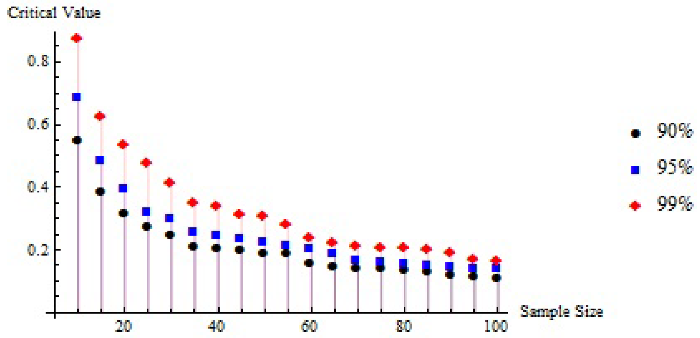
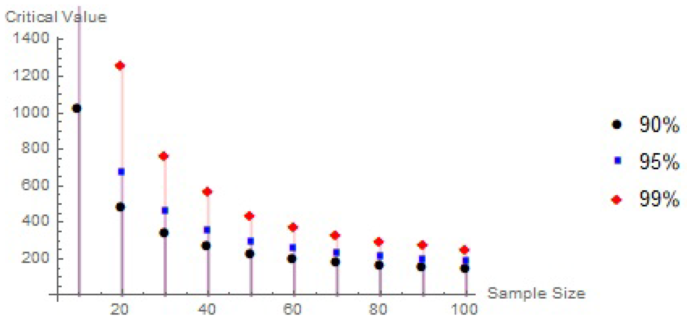
In conclusion, critical values play a pivotal role in statistical testing, providing thresholds for evaluating hypotheses and guiding data-driven decisions. A clear understanding and careful estimation of these values are fundamental for maintaining the accuracy and credibility of statistical findings. This section focuses on simulating critical values under the null hypothesis using Monte Carlo methods, with 10,000 randomly generated samples of sizes ranging from to in increments of 5, implemented in Mathematica 10. The simulations estimate the upper percentiles of , , and at the , , and confidence levels. As demonstrated in Table 3, Table 4 and Table 5 and Figure 1, Figure 2 and Figure 3, the critical values increase with higher confidence levels and tend to decrease as the sample size increases.

Table 3.
The statistic’s critical values of

Table 4.
The statistic’s critical values of

Table 5.
The statistic’s critical values of
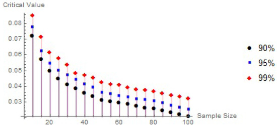
Figure 1.
The correlation between the critical values, sample size, and degree of confidence.
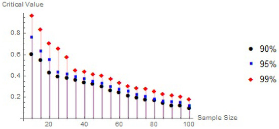
Figure 2.
The correlation between the critical values, sample size, and degree of confidence.

Figure 3.
The correlation between the critical values, sample size, and degree of confidence.
6.2. Estimated Power of the Proposed Test
Power estimates of statistical tests represent the probability that a test will correctly reject the null hypothesis when the alternative hypothesis is true. This measure, known as the power of the test, is a key indicator of the test’s sensitivity and effectiveness in detecting real effects. A high power value, typically or above, suggests that the test is likely to identify a true effect, reducing the risk of a Type II error (failing to reject a false null hypothesis). Power estimates depend on several factors, including the sample size, effect size, variability within the data, and the chosen significance level . In practice, power analysis is often conducted before data collection to determine the required sample size for achieving a desired level of power, thereby ensuring the reliability of the statistical conclusions. Additionally, comparing the power estimates of different tests helps researchers select the most appropriate method for detecting effects under specific conditions, especially in simulation studies or when evaluating test performance across various distributions.
In conclusion, power estimates of statistical tests play a crucial role in the research process, influencing sample size determination, study design, result interpretation, and evidence synthesis across studies. Power analyses improve the rigor and dependability of scientific research by measuring the sensitivity of tests to discover actual effects, thereby advancing knowledge in a variety of domains. The 10,000 samples in Table 5 and Table 6 were used to assess the effectiveness of the proposed test at the confidence level, with . For and 30, assumed values for correspond to the Weibull, Gamma, and LFR distributions, respectively. Table 6, Table 7 and Table 8 show that the , , and tests employed have enough power compared with all other alternatives.

Table 6.
Estimates of the power of

Table 7.
Estimates of the power of

Table 8.
Estimates of the power of
7. Hypothesis Testing Under Censored Data
Testing for censored data is a crucial aspect of statistical analysis, particularly in fields such as survival analysis, reliability engineering, and biomedical research, where complete information on all observations is not always available. Censored data occur when the value of an observation is only partially known, for example, when a study ends before an event occurs or a subject drops out early. This incomplete data poses challenges for traditional statistical methods, which assume fully observed outcomes. As a result, specialized techniques and tests have been developed to handle censoring appropriately, including the Kaplan–Meier estimator, log-rank test, and likelihood-based methods. These methods account for the censored nature of the data, allowing researchers to make valid inferences about population parameters, compare survival distributions, and assess model fit. Proper handling of censored data ensures that statistical conclusions remain accurate and unbiased, preserving the integrity of the analysis despite missing or incomplete information.
An approach for hypothesis testing under censored conditions involves contrasting and using a test statistic derived from randomly right-censored data. In practical scenarios such as clinical trials or reliability studies, such censored observations may be the only information available, especially when subjects drop out or are lost before the completion of the study. The structure of this type of experiment can be formally described as follows: Suppose nn items are under observation, and denote their true lifetimes, assumed to be independent and identically distributed (i.i.d.) from a continuous life distribution F. In parallel, let be i.i.d. censoring times drawn from another continuous distribution G, with the X’s and Y’s assumed independent. The observed data then form the randomly right-censored sample , for , where and
Think of as the ordered series of Z’s, where denotes connected to . With Kaplan and Meier [24] introduced the product limit estimator using the censored data (, ) so that
and
where . To compare with , we suggest using the randomized right-censored data and a test statistic. can be rewritten for computational reasons.
where
and
Test invariance is achieved by letting
Lemma 3
(Scale invariance under independent censoring). Suppose the observed data are with , , and assume independent censoring as above. Let every lifetime be scaled by and, simultaneously, every censoring time be scaled by c. Then the Kaplan–Meier estimate and the plug-in statistic (when normalized by or the mean of the Z’s) are exactly invariant under the common scaling. If only the lifetimes are scaled and the censoring times are unchanged, then under (where the lifetime distribution is exponential with rate λ), scaling by c is equivalent to changing λ to ; because normalization uses the sample mean (or its consistent Kaplan–Meier analog), this change cancels in the limit, and the test statistic is asymptotically invariant provided the Kaplan–Meier mean estimator is consistent and -consistent.
Table 9 and Figure 4 present the critical percentile values for the test derived from the acquired samples . Using Mathematica 10’s conventional exponential distribution with , , and 10,000 replications, critical values for the null Monte Carlo distribution were found. It is evident from Figure 4 and Table 9 that the essential values tend to increase with higher confidence levels and decrease with larger sample sizes.

Table 9.
The superior percentage of with 10,000 replications.
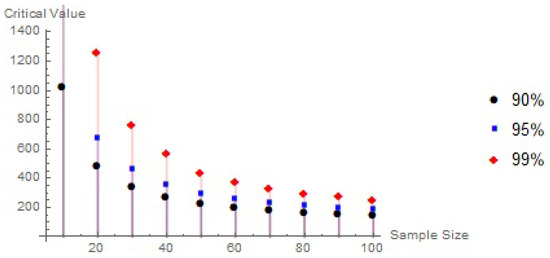
Figure 4.
Relationship among sample size, confidence level, and critical values.
Test Power Estimates
By examining different values of the parameter for 10,000 samples, specifically for sample sizes and 30 in the Weibull, LFR, and Gamma distributions, respectively. The random right censoring was implemented by generating censoring times from an independent exponential distribution, with the rate chosen so that the expected censoring proportion was approximately . This percentage is consistent with typical survival data scenarios and ensures a balance between observed and censored lifetimes. We evaluated the test’s power while maintaining a significance level of . Table 10 shows that all other parameter options had appropriate power estimates using the test .

Table 10.
Estimates of the power of
8. Analysis of Data with Both Censored and Uncensored Observations
Certain types of data present only a partial view, often due to censorship or missing values, which reflect gaps or limitations in the available information. These censored data points can complicate the analytical process, as they require the application of specialized statistical methods and assumptions to extract meaningful insights. In contrast, complete or uncensored data offer a more comprehensive and direct understanding of the phenomenon under study, as they include all relevant observations without restrictions. Analyzing uncensored data is generally more straightforward, allowing for the use of standard techniques and reducing the complexity associated with incomplete datasets. As a result, while censored data present valuable information, they demand more careful handling to ensure accurate and reliable conclusions.
8.1. Non-Censored Data
8.1.1. Dataset I: Polyester Fiber
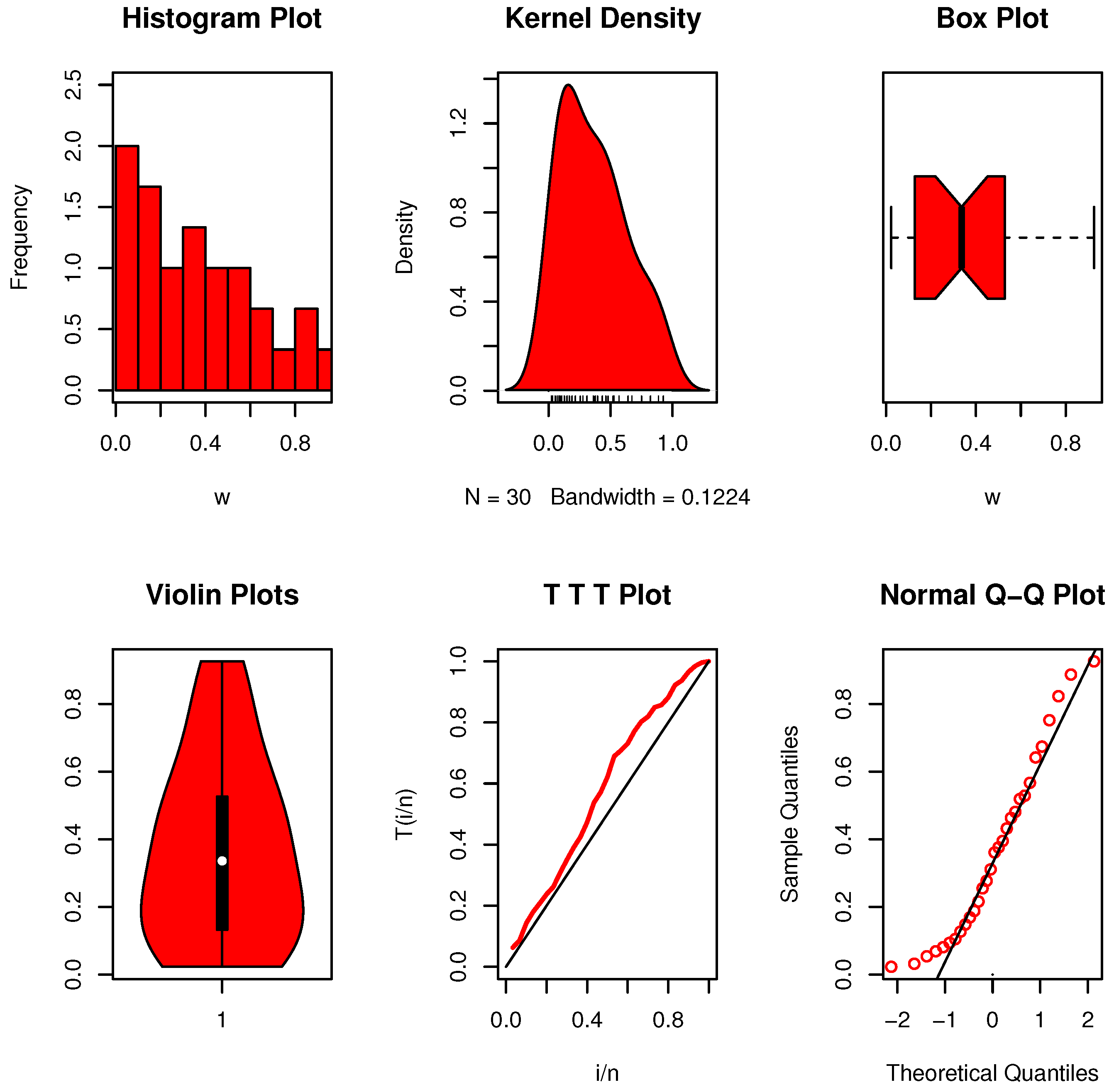
This dataset relates to thirty measurements of the tensile strength of polyester fiber that Al-Omari and Dobbah [25] considered. Here are the observations: 0.023, 0.032, 0.054, 0.069, 0.081, 0.094, 0.105, 0.127, 0.148, 0.169, 0.188, 0.216, 0.255, 0.277, 0.311, 0.361, 0.376, 0.395, 0.432, 0.463, 0.481, 0.519, 0.529, 0.567, 0.642, 0.674, 0.752, 0.823, 0.887, 0.926.
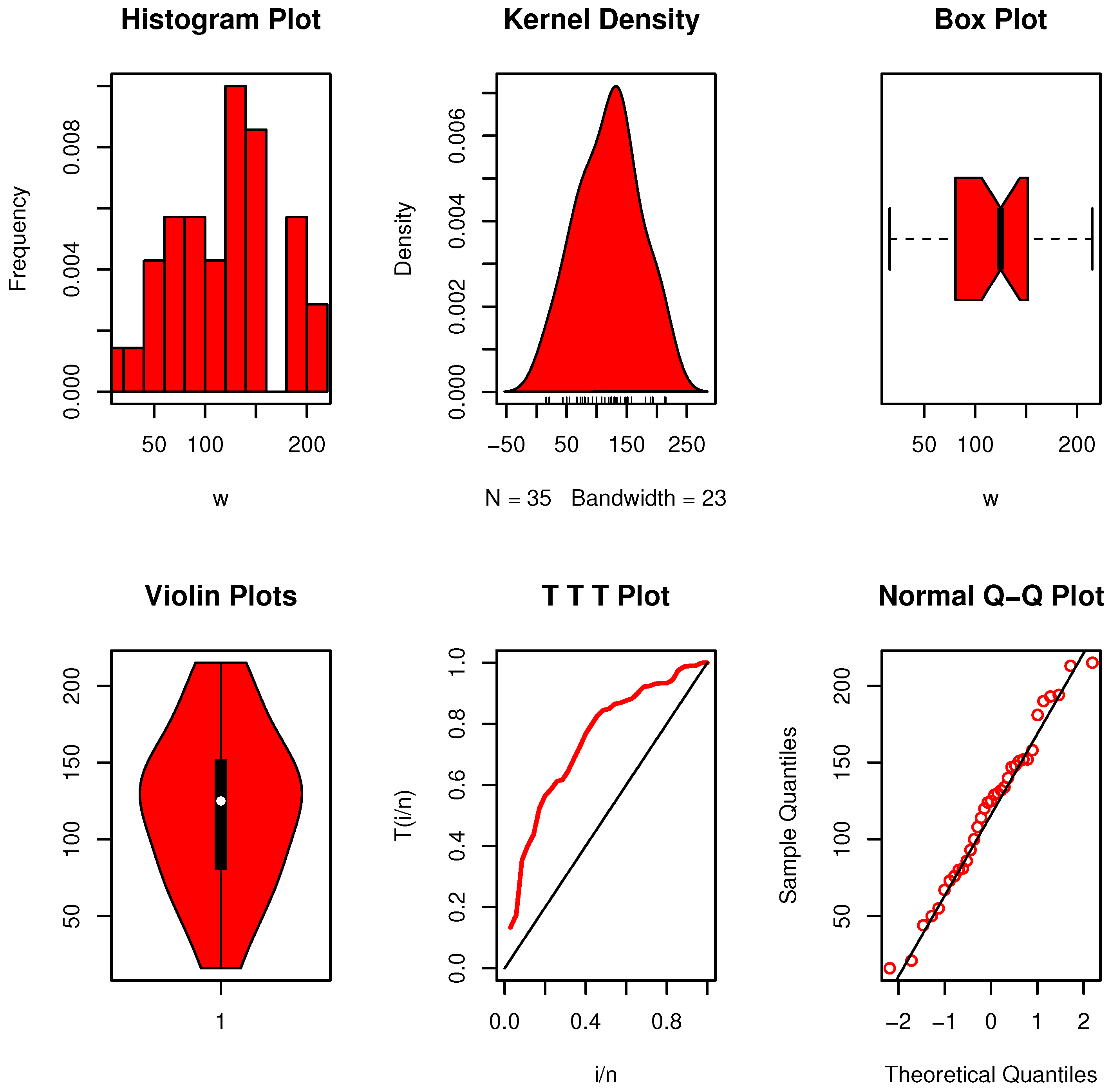
To investigate the characteristics of the data, several nonparametric plots were employed. As illustrated in Figure 5, the distribution is unimodal with slight skewness and no apparent outliers. Moreover, the corresponding hazard function demonstrates a generally increasing pattern. The calculated value, , exceeds the threshold listed in Table 5. This result supports the presence of an EBUCL property within the dataset, leading us to favor this conclusion over the exponential assumption proposed by the alternative hypothesis .

Figure 5.
Nonparametric data visualizations for dataset I.
8.1.2. Dataset II: Electrical Data
Alsadat et al. [26] examined experimental failure time data, recorded in seconds, for two varieties of electrical insulation subjected to a constant voltage load. For each insulation type, thirty samples were collected and evaluated under identical testing conditions.
- The following are type X’s first failure rates: 0.097, 0.014, 0.030, 0.134, 0.240, 0.084, 0.146, 0.024, 0.045, 0.004, 0.099, 0.277, 0.472, 0.094, 0.023, 0.146, 0.030, 0.031, 0.104, 0.105, 0.036, 0.065, 0.022, 0.098, 0.178, 0.059, 0.014, 0.007, 0.007, 0.286.
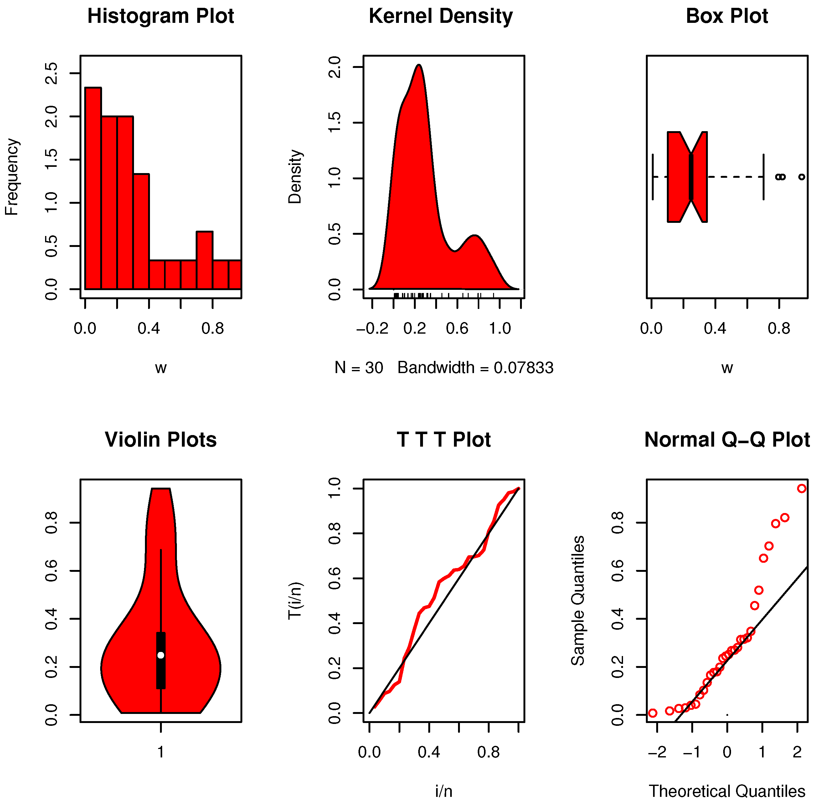
- The failure rates of the second type Y are as follows: 0.084, 0.236, 0.315, 0.199, 0.252, 0.103, 0.455, 0.135, 0.348, 0.321, 0.166, 0.040, 0.027, 0.519, 0.017, 0.821, 0.942, 0.270, 0.008, 0.030, 0.177, 0.268, 0.180, 0.796, 0.245, 0.703, 0.045, 0.314, 0.281, 0.652.
Figure 6 shows nonparametric plots for dataset II-X. The distribution appears multimodal and positively skewed, with no extreme outliers. Figure 7 displays the plots for dataset II-Y. The distribution is also multimodal but more spread out and asymmetrical. When comparing our determined conclusion, , to the crucial value in Table 5, it is evident that the data (type X) has an exponential character. The critical value for data type Y, on the other hand, is exceeded by , as shown in Table 5. As indicated in , this implies that the data collection exhibits an characteristic rather than exponential development, which we subsequently agree with.
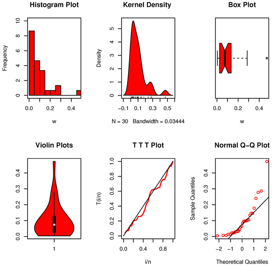
Figure 6.
Nonparametric data visualizations for dataset II-X.
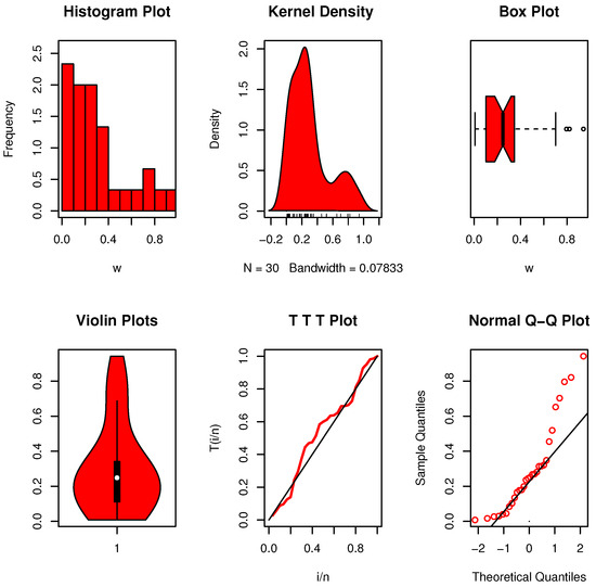
Figure 7.
Nonparametric data visualizations for dataset II-Y.
8.1.3. Dataset III: The Long Glass Fibers
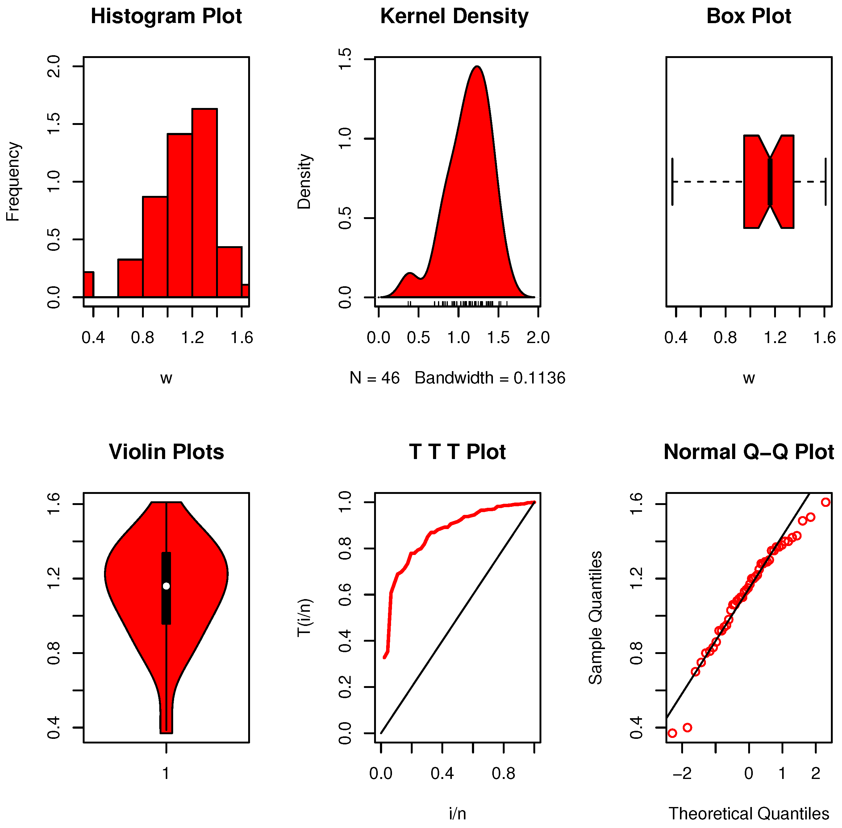
This collection of experimental data on the strength of 15 cm long glass fibers comes from Meintanis et al. [27]. The 46 observations listed below provide the observations: 0.37, 0.40, 0.70, 0.75, 0.80, 0.81, 0.83, 0.86, 0.92, 0.92, 0.94, 0.95, 0.98, 1.03, 1.06, 1.06, 1.08, 1.09, 1.10, 1.10, 1.13, 1.14, 1.15, 1.17, 1.20, 1.20, 1.21, 1.22, 1.25, 1.28, 1.28, 1.29, 1.29, 1.30, 1.35, 1.35, 1.37, 1.37, 1.38, 1.40, 1.40, 1.42, 1.43, 1.51, 1.53, 1.61.
Figure 8 presents the plots for dataset III (Long Glass Fibers). The data show a clear multimodal distribution with a slight right skew. In this instance, the calculated value, , is above the critical limit stated in Table 5. This implies that rather than the exponential development that claimed, the data collection exhibits an EBUCL feature, which we subsequently accept.

Figure 8.
Nonparametric data visualizations for dataset III.
8.1.4. Dataset IV: Strengths of Glass Fibers
Replicating the strengths of glass fibers is the aim of this data gathering. The dataset that Ahmad et al. [28] acquired is as follows: 1.014, 1.248, 1.267, 1.271, 1.272, 1.275, 1.276, 1.355, 1.361, 1.364, 1.379, 1.409, 1.426, 1.459, 2.456, 2.592, 1.292, 1.081, 1.082, 1.185, 1.223, 1.304, 1.306, 1.46, 1.476, 1.481, 1.484, 1.501, 1.506, 1.524, 1.526, 1.535, 1.541, 1.568, 1.735, 1.278, 1.286, 1.288, 1.867, 1.876, 1.878, 1.91, 1.916, 1.972, 2.012, 1.747, 1.748, 1.757, 1.8, 1.579, 1.581, 1.591, 1.593, 1.602, 1.666, 1.67, 1.684, 1.691, 1.704, 1.731, 1.806, 3.197, 4.121.
Figure 9 indicates that the data exhibit a slightly skewed, multimodal distribution with noticeable extreme values. The plots also suggest that the data are not symmetrically shaped. Moreover, the associated hazard function demonstrates an upward trend. The calculated value in this instance, , is higher than the critical limit shown in Table 5. This claim is accurate since, at the significance level, the data also meet the EBUCL feature requirements.
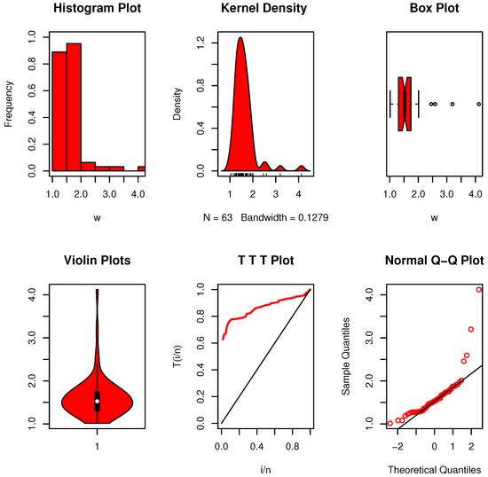
Figure 9.
Nonparametric data visualizations for dataset IV.
8.1.5. Dataset V: Breaking Stress
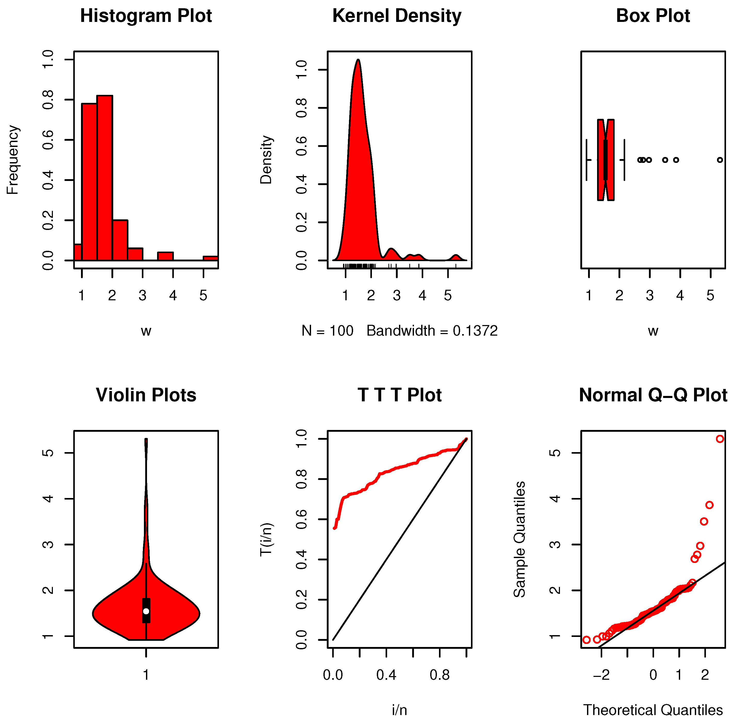
A dataset from Ahmad et al.’s [28] study on the breaking stress of 100 carbon fibers (in Gba) was analyzed. The lifespans are the amounts of time that pass before the fibers break: “0.92, 0.928, 0.997, 0.9971, 1.061, 1.117, 1.162, 1.183, 1.187, 1.192, 1.196, 1.213, 1.215, 1.2199, 1.22, 1.224, 1.225, 1.228, 1.237, 1.24, 1.244, 1.259, 1.261, 1.263, 1.276, 1.31, 1.321, 1.329, 1.331, 1.337, 1.351, 1.359, 1.388, 1.408, 1.449, 1.4497, 1.45, 1.459, 1.471, 1.475, 1.477, 1.48, 1.489, 1.501, 1.507, 1.515, 1.53, 1.5304, 1.533, 1.544, 1.5443, 1.552, 1.556, 1.562, 1.566, 1.585, 1.586, 1.599, 1.602, 1.614, 1.616, 1.617, 1.628, 1.684, 1.711, 1.718, 1.733, 1.738, 1.743, 1.759, 1.777, 1.794, 1.799, 1.806, 1.814, 1.816, 1.828, 1.83, 1.884, 1.892, 1.944, 1.972, 1.984, 1.987, 2.02, 2.0304, 2.029, 2.035, 2.037, 2.043, 2.046, 2.059, 2.111, 2.165, 2.686, 2.778, 2.972, 3.504, 3.863, 5.306”.
Figure 10 shows that the data possess a moderately skewed, multimodal distribution with some extreme values present. The visual patterns confirm that the distribution lacks symmetry. In addition, the hazard function reveals an increasing trend, reflecting a growing likelihood of failure as time progresses. The calculated value in this instance, , is more than the crucial threshold shown in Table 5. This is accurate, as this specific data type satisfies the EBUCL characteristic at the significance level of .
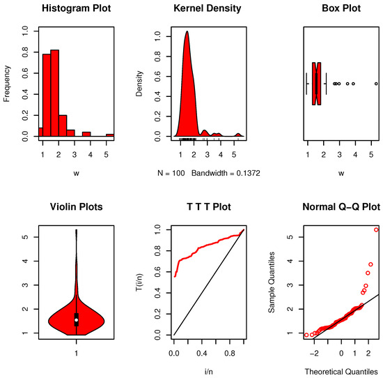
Figure 10.
Nonparametric data visualizations for dataset V.
8.1.6. Dataset VI: Tensile Strength
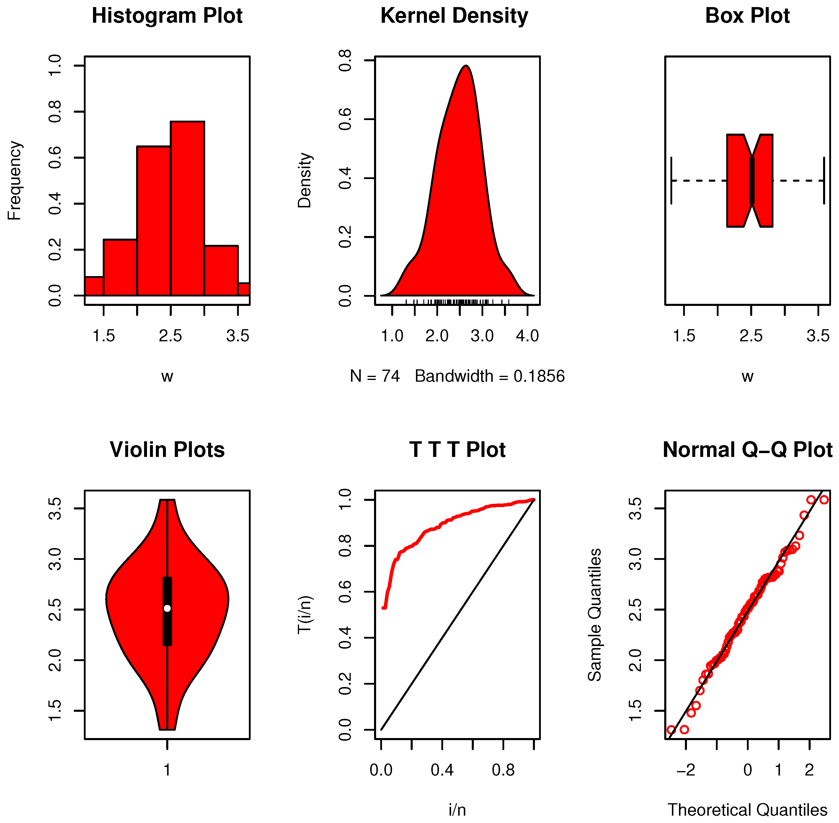
Because of its excellent tensile strength, low density, electrical conductivity, chemical stability, and high thermal conductivity, carbon fiber was widely employed in the industry. Fibers are therefore employed nowadays to create a number of components that are required to be strong and lightweight. In this application, the strength of impregnated thousand-carbon fibers and single-carbon fibers, measured in gigapascal (GPa) at gauge lengths of 20 mm, under stress is investigated. This data was addressed by Ahmad et al. [29] and is displayed below: 1.312, 1.314, 1.479, 1.552, 1.7, 1.803, 1.861, 1.865, 1.944, 1.958, 1.966, 1.997, 2.006, 2.021, 2.027, 2.055, 2.063, 2.098, 2.14, 2.179, 2.224, 2.24, 2.253, 2.27, 2.272, 2.274, 2.301, 2.301, 2.359, 2.382, 2.426, 2.434, 2.435, 2.382, 2.478, 2.554, 2.514, 2.511, 2.49, 2.535, 2.566, 2.57, 2.586, 2.629, 2.8, 2.773, 2.77, 2.809, 3.585, 2.818, 2.642, 2.726, 2.697, 2.684, 2.648, 2.633, 3.128, 3.09, 3.096, 3.233, 2.821, 2.88, 2.848, 2.818, 3.067, 2.821, 2.954, 2.809, 3.585, 3.084, 3.012, 2.88, 2.848, 3.433.
Figure 11 illustrates that the data follow a unimodal distribution, with no apparent outliers and a fairly symmetric shape. The nonparametric plots support the absence of skewness or irregularities. Moreover, the hazard function indicates an upward trend. The calculated value in this instance, , is more than the crucial threshold shown in Table 5. This is accurate, as this specific data type satisfies the EBUCL characteristic at the significance level of .

Figure 11.
Nonparametric data visualizations for dataset VI.
8.1.7. Dataset VII: Glass Fiber Strengths
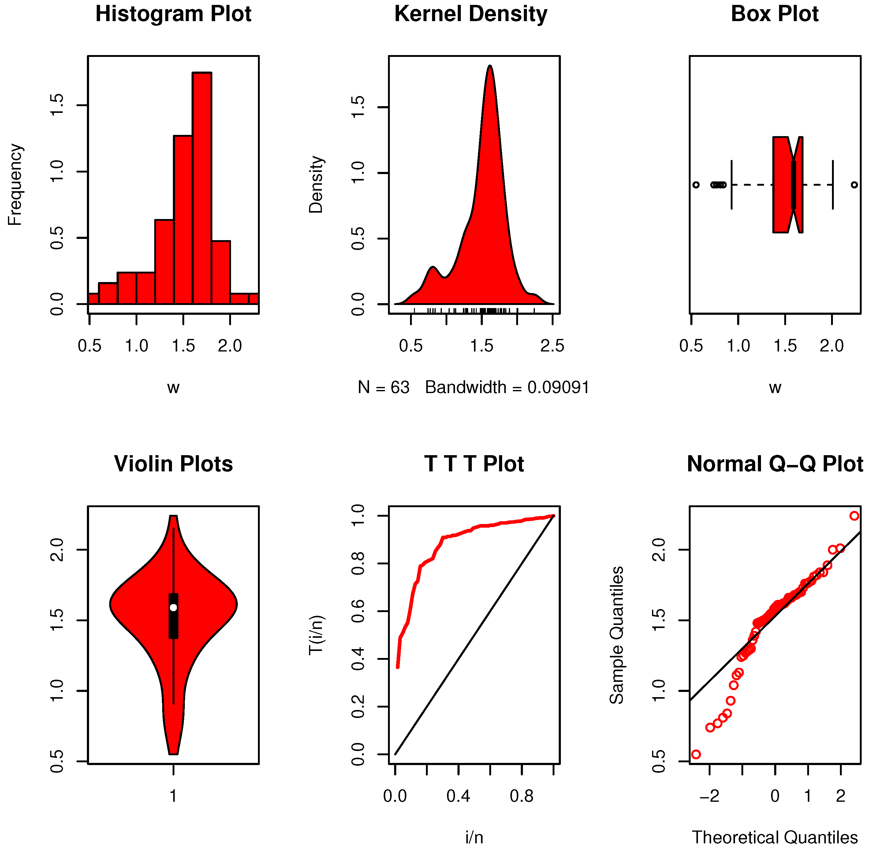
Ekemezie et al. [30] examined the dataset, which includes 63 observations of 1.5 cm glass fiber strengths obtained at the National Physical Laboratory in England. The data is “0.55, 0.74, 0.77, 0.81, 0.84, 0.93, 1.04, 1.11, 1.13, 1.24, 1.25, 1.27, 1.28, 1.29, 1.30, 1.36, 1.39, 1.42, 1.48, 1.48, 1.49, 1.49, 1.50, 1.50, 1.51, 1.52, 1.53, 1.54, 1.55, 1.55, 1.58, 1.59, 1.60, 1.61, 1.61, 1.61, 1.61, 1.62, 1.62, 1.63, 1.64, 1.66, 1.66, 1.66, 1.67, 1.68, 1.68, 1.69, 1.70, 1.70, 1.73, 1.76, 1.76, 1.77, 1.78, 1.81, 1.82, 1.84, 1.84, 1.89, 2.00, 2.01, 2.24”.
Figure 12 demonstrates that the data follow a multimodal distribution, display no significant outliers, and have an asymmetrical structure. The shape of the plots confirms the lack of symmetry. Furthermore, the hazard rate shows an increasing pattern. Table 5’s critical limit is substantially lower than the calculated value in this instance, . The EBUCL feature is satisfied by this particular data type at the significance level of ; hence, this is correct.

Figure 12.
Nonparametric data visualizations for dataset VII.
8.1.8. Dataset VIII: Carbon Fibers
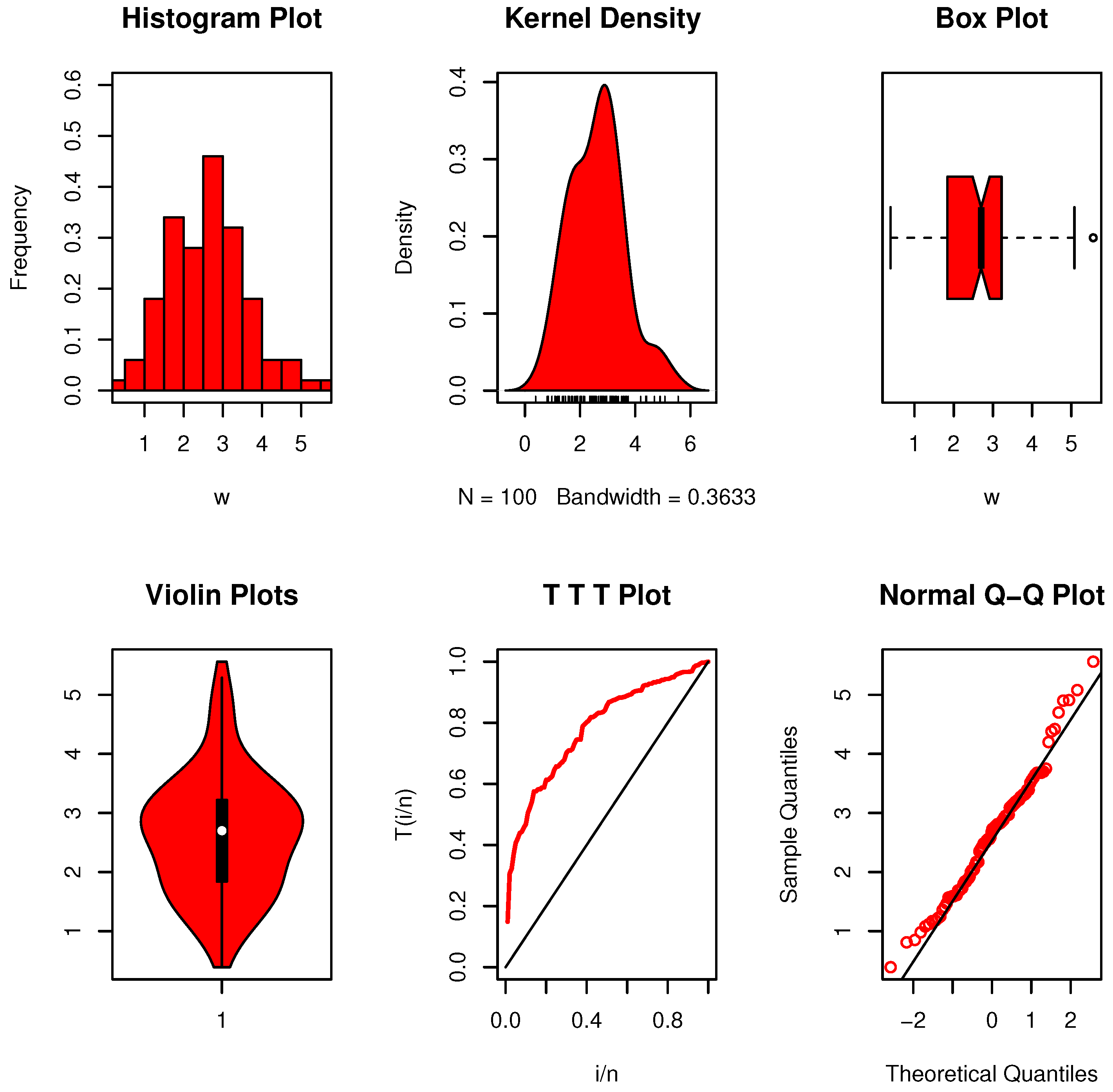
One hundred unedited observations measuring the breaking stress of carbon fibers, expressed in gigapascals (GPa), make up the dataset under review. Shehata et al. [31] published these results, which are a useful tool for researching the mechanical characteristics of carbon fibers under stress. Because carbon fibers are strong and lightweight, they are utilized extensively in industries like aerospace and automotive, where it is essential to understand their breaking stress. The data is 3.70, 2.74, 2.73, 2.50, 3.60, 3.11, 3.27, 2.87, 1.47, 3.11, 4.42, 2.41, 3.19, 3.22, 1.69, 3.28, 3.09, 1.87, 3.15, 4.90, 3.75, 2.43, 2.95, 2.97, 3.39, 2.96, 2.53, 2.67, 2.93, 3.22, 3.39, 2.81, 4.20, 3.33, 2.55, 3.31, 3.31, 2.85, 2.56, 3.56, 3.15, 2.35, 2.55, 2.59, 2.38, 2.81, 2.77, 2.17, 2.83, 1.92, 1.41, 3.68, 2.97, 1.36, 0.98, 2.76, 4.91, 3.68, 1.84, 1.59, 3.19, 1.57, 0.81, 5.56, 1.73, 1.59, 2.00, 1.22, 1.12, 1.71, 2.17, 1.17, 5.08, 2.48, 1.18, 3.51, 2.17, 1.69, 1.25, 4.38, 1.84, 0.39, 3.68, 2.48, 0.85, 1.61, 2.79, 4.70, 2.03, 1.80, 1.57, 1.08, 2.03, 1.61, 2.12, 1.89, 2.88, 2.82, 2.05, 3.65.
To examine the properties of the data, nonparametric plots were generated. Figure 13 reveals that the data exhibit a unimodal distribution, are free from extreme values, and display a moderately asymmetric shape. Furthermore, the hazard rate indicates an increasing pattern over time. The calculated value in this instance exceeds the critical limit shown in Table 5. This implies that rather than the exponential development that claimed, the data collection exhibits an EBUCL feature, which we subsequently accept.
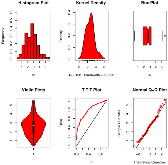
Figure 13.
Nonparametric data visualizations for dataset VIII.
8.2. Censored Data
8.2.1. Dataset IX: Lung Cancer
Consider the dataset provided by Yu and Zhang [32], which presents the survival times, in weeks, of 61 patients diagnosed with terminal lung cancer and treated with cyclophosphamide. Among these patients, treatment was halted for some due to deteriorating health, resulting in 28 censored observations and 33 uncensored ones:
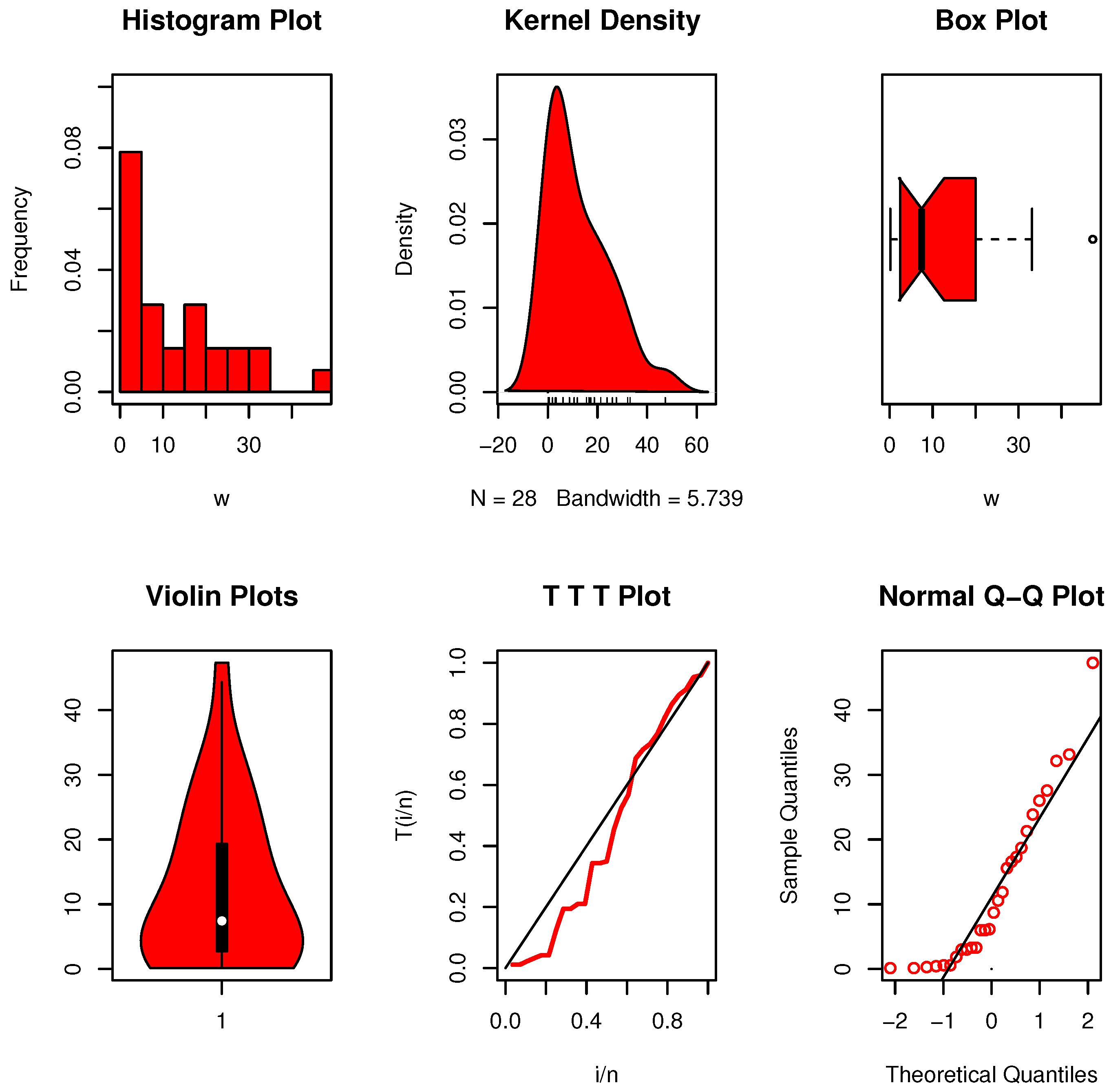
- Censored observations: 0.14, 0.14, 0.29, 0.43, 0.57, 0.57, 1.86, 3, 3, 3.29, 3.29, 6, 6, 6.14, 8.71, 10.57, 11.86, 15.57, 16.57, 17.29, 18.71, 21.29, 23.86, 26, 27.57, 32.14, 33.14, 47.29.
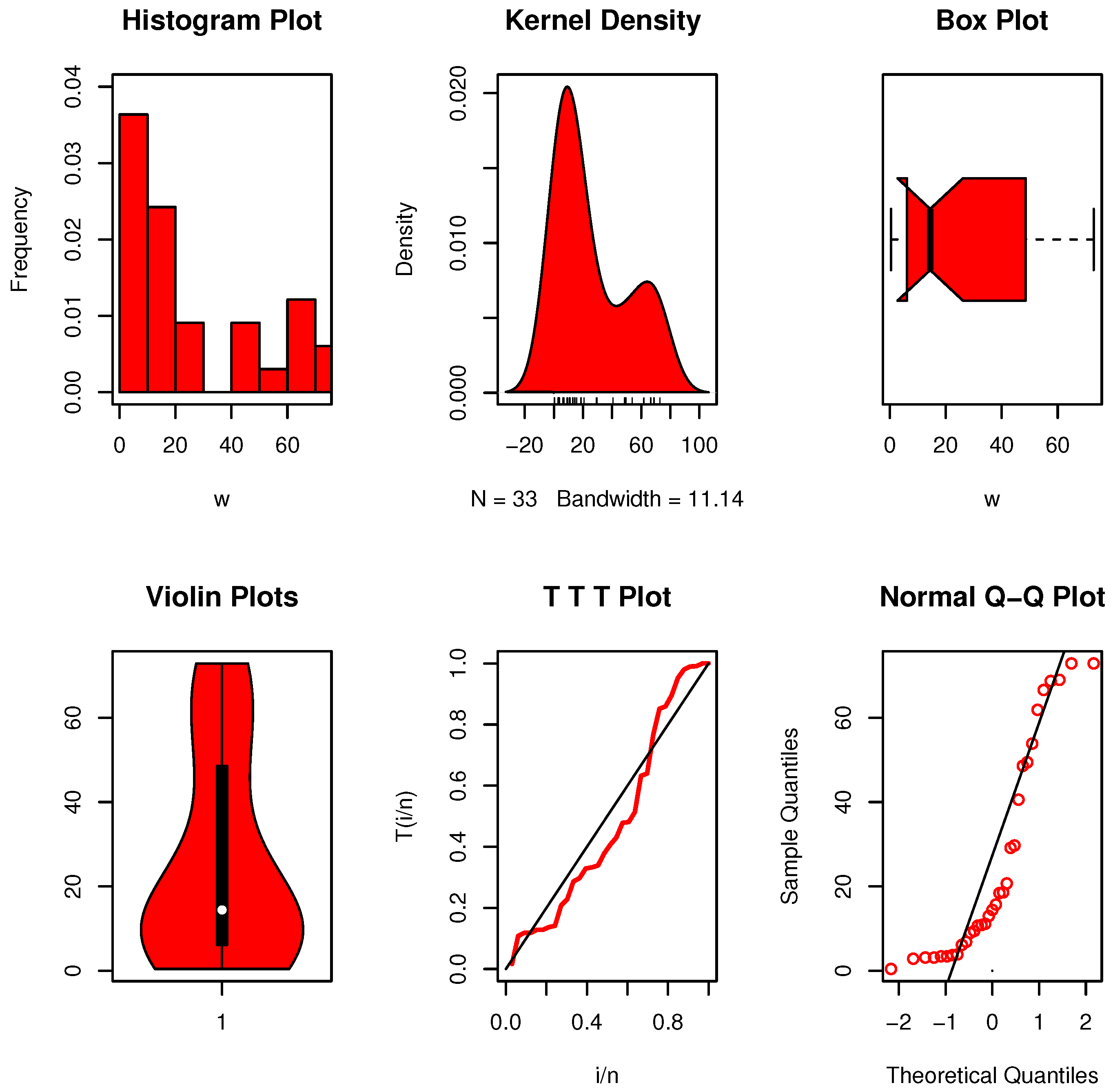
- Uncensored observations: 0.43, 2.86, 3.14, 3.14, 3.43, 3.43, 3.71, 3.86, 6.14, 6.86, 9, 9.43, 10.71, 10.86, 11.14, 13, 14.43, 15.71, 18.43, 18.57, 20.71, 29.14, 29.71, 40.57, 48.57, 49.43, 53.86, 61.86, 66.57, 68.71, 68.96, 72.86, 72.86.
The data visualization plots are presented in Figure 14 and Figure 15. The analysis reveals the presence of extreme observations, and the nucleation intensity is skewed towards the right. Upon considering the remaining data, both censored and uncensored, Table 9 demonstrates that the crucial value, , is greater than our estimate. The data are exponential as a result.

Figure 14.
Nonparametric data visualizations for dataset IX-A.

Figure 15.
Nonparametric data visualizations for dataset IX-B.
8.2.2. Dataset X: Melanoma Patient
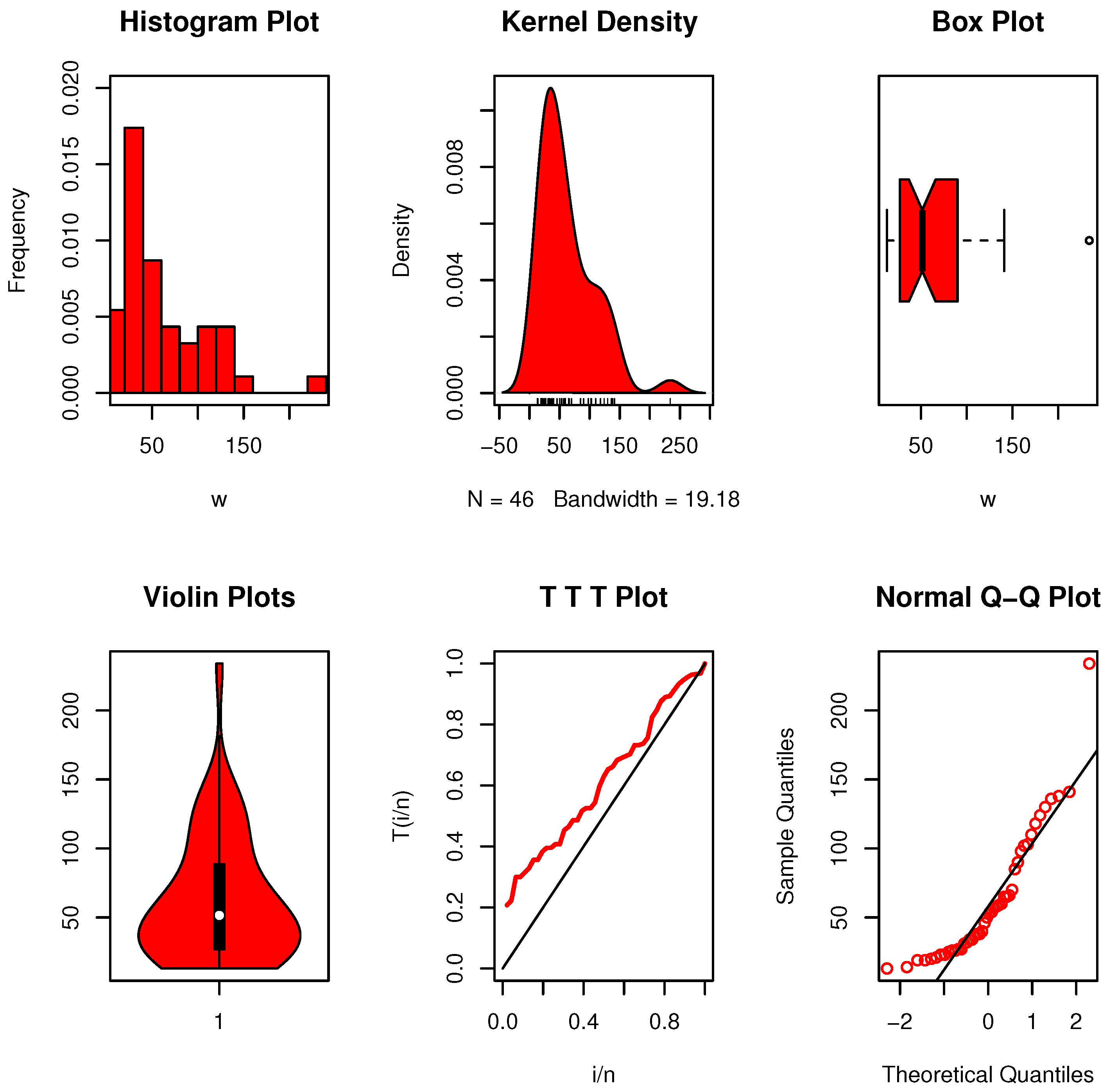
Take Das and Ghosh’s [33] data as an example. Forty-six melanoma patient survival rates are displayed in these statistics. Thirty-five of them represent full lives (non-censored data). The following is a list of the suppressed observations. The data is 13, 14, 19, 19, 20, 21, 23, 23, 25, 26, 26, 27, 27, 31, 32, 34, 34, 37, 38, 38, 40, 46, 50, 53, 54, 57, 58, 59, 60, 65, 65, 66, 70, 85, 90, 98, 102, 103, 110, 118, 124, 130, 136, 138, 141, 234 (Figure 16).
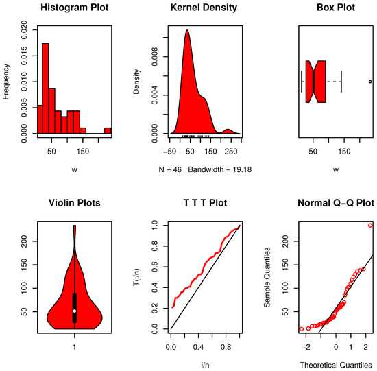
Figure 16.
Nonparametric data visualizations for dataset X-A.
The following sequence applies to the suppressed observations: 16, 21, 44, 50, 55, 67, 73, 76, 80, 81, 86, 93, 100, 108, 114, 120, 124, 125, 129, 130, 132, 134, 140, 147, 148, 151, 152, 152, 158, 181, 190, 193, 194, 213, 215.
Figure 17 indicates that the data follow a unimodal distribution, with no apparent extreme values, and display an asymmetric shape. In addition, the hazard rate shows a clear increasing trend. If we take into account all of the survival statistics, both filtered and uncensored. We derive , which is less than Table 9’s critical value. Consequently, we recognize that this data exhibits exponential characteristics.
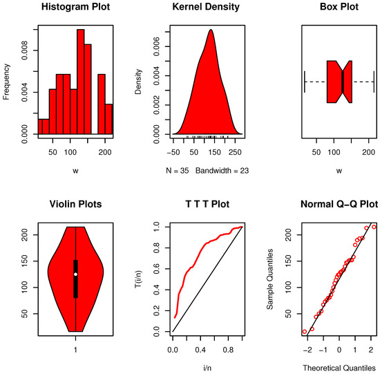
Figure 17.
Nonparametric data visualizations for dataset X-B.
9. Conclusions
Reliability refers to the consistency of measurements or system performance over time and is crucial for the development of effective testing methods and analytical tools. In statistics and engineering, reliable results ensure meaningful comparisons across datasets and enhance the credibility of conclusions. While reliability focuses on consistency, validity pertains to the accuracy of the measurements, highlighting that a test can be reliable without necessarily being valid. In industrial engineering, reliability is associated with a system’s ability to perform its intended function efficiently over an extended period, despite the complexity of modern systems composed of interdependent components. The failure of a single part can compromise the entire system, making reliability analysis essential. This has led to the development of reliability theory, which emphasizes the quantification and evaluation of product performance. Additionally, foundational concepts such as symmetry, asymmetry, and stochastic ordering of probability distributions play a key role in fields like reliability, survival analysis, and economics. This study introduced a new nonparametric test for assessing exponentiality against the recently defined EBUCL class of life distributions. The test was constructed using Laplace transform ordering and demonstrated strong theoretical properties, including asymptotic normality and high Pitman asymptotic efficiency under various alternatives such as Weibull, Makeham, and LFR distributions. In selecting the alternatives and their parameters, our intention was to ensure both theoretical relevance and practical representativeness. The Weibull, Makeham, linear failure rate (LFR), and Gamma distributions were chosen because they constitute standard benchmarks in the literature on exponentiality testing and are frequently encountered in reliability and survival analysis. Their parameter values were specified to capture a spectrum of departures from exponentiality: for example, the Weibull with a shape parameter of 2 reflects a monotone increasing hazard, while the Gamma with a shape parameter of ≥3 provides heavier-tailed behavior. These settings enable us to evaluate the proposed test not only under strong alternatives, which emphasize the test’s power, but also under moderate deviations commonly observed in applied data. The parameter choices are further guided by Pitman’s asymptotic efficiency analysis, ensuring that the scenarios examined are theoretically informative as well as practically meaningful. Through extensive Monte Carlo simulations, critical values were obtained, and the power of the proposed test was shown to surpass several existing methods. Additionally, the test was successfully extended to accommodate right-censored data, ensuring its applicability in survival and reliability analyses. Empirical applications to a variety of real-world datasets, both censored and uncensored, further confirmed the robustness and versatility of the proposed method. For each dataset, we report the standardized statistic, the p-value, and a clear decision: “At the significance level, we reject in favor of ” (or “do not reject ”). This conforms to standard statistical reporting. The findings validate the practical utility of the test in detecting deviations from exponentiality and support its relevance in engineering, medical, and actuarial sciences.
Author Contributions
Conceptualization, O.S.B. and R.M.E.-S.; Methodology, W.B.H.E., M.E.B., A.M.A., O.S.B., and R.M.E.-S.; Software, W.B.H.E. and R.M.E.-S.; Validation, W.B.H.E., M.E.B., O.S.B., and R.M.E.-S.; Formal analysis, M.E.B., A.M.A., and R.M.E.-S.; Investigation, W.B.H.E., A.M.A., and R.M.E.-S.; Resources, W.B.H.E., M.E.B., A.M.A., and O.S.B.; Data curation, M.E.B., A.M.A., O.S.B., and R.M.E.-S.; Writing—original draft, W.B.H.E. and A.M.A.; Writing—review and editing, R.M.E.-S.; Visualization, M.E.B. and O.S.B.; Supervision, A.M.A. and R.M.E.-S.; Funding acquisition, A.M.A. All authors have read and agreed to the published version of the manuscript.
Funding
Ongoing Research Funding program, (ORF-2025-1004), King Saud University, Riyadh, Saudi Arabia.
Data Availability Statement
The original contributions presented in this study are included in the article. Further inquiries can be directed to the corresponding author.
Acknowledgments
This study was funded by Ongoing Research Funding program, (ORF-2025-1004), King Saud University, Riyadh, Saudi Arabia.
Conflicts of Interest
The authors declare no conflicts of interest.
References
- Bryson, M.C.; Siddiqui, M.M. Some criteria for ageing. Am. Stat. Assoc. 1969, 64, 1472–1483. [Google Scholar] [CrossRef]
- Barlow, R.E.; Proschan, F. Statistical Theory of Reliability and Life Testing; Hold, Reinhart and Wiston, Inc.: Silver Spring, MD, USA, 1981. [Google Scholar]
- Klefsjo, B. The HNBUE and HNWUE classes of life distributions. Nav. Res. Logist. Q. 1982, 29, 331–344. [Google Scholar] [CrossRef]
- Kumazawa, Y. A class of tests statistics for testing whether new is better than used. Commun. Stat.-Theory Methods 1983, 12, 311–321. [Google Scholar] [CrossRef]
- Cuparić, M.; Milošević, B. New characterization-based exponentiality tests for randomly censored data. Test 2022, 31, 461–487. [Google Scholar] [CrossRef]
- Hassan, N.A.; Said, M.M.; Attwa, R.A.E.W.; Radwan, T. Applying the Laplace transform procedure, testing exponentiality against the NBRUmgf class. Mathematics 2024, 12, 2045. [Google Scholar] [CrossRef]
- Etman, W.B.; Bakr, M.E.; Balogun, O.S.; EL-Sagheer, R.M. A novel statistical test for life distribution analysis: Assessing exponentiality against EBUCL class with applications in sustainability and reliability data. Axioms 2025, 14, 140. [Google Scholar] [CrossRef]
- Etman, W.B.; Eliwa, M.S.; Alqifari, H.N.; El-Morshedy, M.; Al-Essa, L.A.; EL-Sagheer, R.M. The NBRULC reliability class: Mathematical theory and goodness-of-fit testing with applications to asymmetric censored and uncensored data. Mathematics 2023, 11, 2805. [Google Scholar] [CrossRef]
- Mohamed, N.M.; Mansour, M.M.M. Testing exponentiality against NBUC class with some applications in health and engineering fields. Front. Sci. Res. Technol. 2024, 8, 90–97. [Google Scholar] [CrossRef]
- El-Arishy, S.M.; Diab, L.S.; El-Atfy, E.S. Characterizations on decreasing laplace transform of time to failure class and hypotheses testing. J. Comput. Sci. Comput. 2020, 10, 49–54. [Google Scholar] [CrossRef]
- Gadallah, A.M. Testing EBUmgf class of life distributions based on Laplace transform technique. J. Stat. Probab. 2017, 6, 471–477. [Google Scholar]
- Abu-Youssef, S.E.; El-Toony, A.A. A new class of life distribution based on Laplace transform and it’s applications. Inf. Sci. Lett. 2022, 11, 355–362. [Google Scholar] [CrossRef]
- Bakr, M.E.; Al-Babtain, A.A. Non-parametric hypothesis testing for unknown aged class of life distribution using real medical data. Axioms 2023, 12, 369. [Google Scholar] [CrossRef]
- Atallah, M.A.; Mahmoud, M.A.W.; Alzahrani, B.M. A new test for exponentiality versus NBUmgf life distribution based on Laplace transform. Qual. Reliab. Eng. Int. 2014, 30, 1353–1359. [Google Scholar] [CrossRef]
- Al-Gashgari, F.H.; Shawky, A.I.; Mahmoud, M.A.W. A non-parametric test for exponentiality against NBUCA class of life distribution based on Laplace transform. Qual. Reliab. Int. 2016, 32, 29–36. [Google Scholar] [CrossRef]
- Abu-Youssef, S.E.; Ali, N.S.A.; El-Toony, A.A. Nonparametric test for a class of lifetime distribution UBAC(2) based on the Laplace transform. J. Egypt. Math. Soc. 2022, 30, 9. [Google Scholar] [CrossRef]
- Mansour, M.M.M. Assessing treatment methods via testing exponential property for clinical data. J. Stat. Probab. 2022, 11, 109–113. [Google Scholar]
- Mansour, M.M.M. Non-parametric statistical test for testing exponentiality with applications in medical research. Stat. Med. Res. 2019, 29, 413–420. [Google Scholar] [CrossRef]
- Abu-Youssef, S.E.; Bakr, M.E. Laplace transform order for unknown age class of life distribution with some applications. J. Stat. Appl. Probab. 2018, 7, 105–114. [Google Scholar] [CrossRef]
- Lee, A.J. U-Statistics; Marcel Dekker: New York, NY, USA, 1989. [Google Scholar]
- Pitman, E.J.G. Some Basic Theory for Statistical Inference; Chapman & Hall: London, UK, 1979. [Google Scholar]
- Mugdadi, A.R.; Ahmad, I.A. Moment inequalities derived from comparing life with its equilibrium form. J. Stat. Inference 2005, 134, 303–317. [Google Scholar]
- Kango, A.I. Testing for new is better than used. Commun. Stat.-Theory Methods 1993, 12, 311–321. [Google Scholar]
- Kaplan, E.L.; Meier, P. Nonparametric estimation from incomplete observation. J. Am. Stat. 1958, 53, 457–481. [Google Scholar] [CrossRef]
- Al-Omari, A.I.; Dobbah, S.A. On the mixture of Shanker and gamma distributions with applications to engineering data. J. Radiat. Res. Appl. Sci. 2023, 16, 100533. [Google Scholar] [CrossRef]
- Alsadat, N.; Almetwally, E.M.; Elgarhy, M.; Ahmad, H.; Marei, G.A. Bayesian and non-Bayesian analysis with MCMC algorithm of stress-strength for a new two parameters lifetime model with applications. AIP Adv. 2023, 13, 095203. [Google Scholar] [CrossRef]
- Meintanis, S.G.; Milošević, B.; Jiménez–Gamero, M.D. Goodness-of-fit tests based on the min-characteristic function. Comput. Stat. Data Anal. 2024, 197, 107988. [Google Scholar] [CrossRef]
- Ahmad, A.; Alghamdi, F.M.; Ahmad, A.; Albalawi, O.; Zaagan, A.A.; Zakarya, M.; Almetwally, E.M.; Mekiso, G.T. New Arctan-generator family of distributions with an example of Frechet distribution: Simulation and analysis to strength of glass and carbon fiber data. Alex. Eng. J. 2024, 100, 42–52. [Google Scholar] [CrossRef]
- Ahmad, H.H.; Abo-Kasem, O.E.; Rabaiah, A.; Elshahhat, A. Survival analysis of newly extended Weibull data via adaptive progressive Type-II censoring and its modeling to Carbon fiber and electromigration. AIMS Math. 2025, 10, 10228–10262. [Google Scholar] [CrossRef]
- Ekemezie, D.F.N.; Alghamdi, F.M.; Aljohani, H.M.; Riad, F.H.; Abd El-Raouf, M.M.; Obulezi, O.J. A more flexible Lomax distribution: Characterization, estimation, group acceptance sampling plan and applications. Alex. Eng. J. 2024, 109, 520–531. [Google Scholar] [CrossRef]
- Shehata, W.A.; Aljadani, A.; Mansour, M.M.; Alrweili, H.; Hamed, M.S.; Yousof, H.M. A novel reciprocal-Weibull model for extreme reliability data: Statistical properties, reliability applications, reliability PORT-VaR and mean of order P risk analysis. Pak. Stat. Oper. Res. 2024, 20, 693–718. [Google Scholar] [CrossRef]
- Yu, H.; Zhang, L. Copula-based semiparametric nonnormal transformed linear model for survival data with dependent censoring. J. Stat. Plan. Inference 2025, 240, 106296. [Google Scholar] [CrossRef]
- Das, K.; Ghosh, S. A class of nonparametric tests for DMTTF alternatives based on moment inequality. Stat. Pap. 2025, 66, 47. [Google Scholar] [CrossRef]
Disclaimer/Publisher’s Note: The statements, opinions and data contained in all publications are solely those of the individual author(s) and contributor(s) and not of MDPI and/or the editor(s). MDPI and/or the editor(s) disclaim responsibility for any injury to people or property resulting from any ideas, methods, instructions or products referred to in the content. |
© 2025 by the authors. Licensee MDPI, Basel, Switzerland. This article is an open access article distributed under the terms and conditions of the Creative Commons Attribution (CC BY) license (https://creativecommons.org/licenses/by/4.0/).


