Article

Robust Bias Compensation LMS Algorithms Under Colored Gaussian Input Noise and Impulse Observation Noise Environments

1
Department of Electronic Engineering, National Taipei University of Technology, Taipei 10608, Taiwan
2
Department of Electrical Engineering, National Ilan University, Yilan 26047, Taiwan
3
College of Electronic and Information Engineering, Southwest University, Chongqing 400715, China
*
Author to whom correspondence should be addressed.
Mathematics 2025, 13(20), 3348; https://doi.org/10.3390/math13203348
Submission received: 16 September 2025 / Revised: 15 October 2025 / Accepted: 17 October 2025 / Published: 21 October 2025

Abstract

Adaptive filtering algorithms often suffer from biased parameter estimation and performance degradation in the presence of colored input noise and impulsive observation noise, both of which are common in practical sensor and communication systems. Existing bias-compensated least mean square (LMS) algorithms generally assume white Gaussian input noise, thereby limiting their applicability in real-world scenarios. This paper introduces a robust convex combination bias-compensated LMS (CC-BC-LMS) algorithm designed to address both colored Gaussian input noise and impulsive observation noise. The proposed algorithm achieves bias compensation through robust estimation of the input noise autocorrelation matrix and employs a modified Huber function to mitigate the influence of impulsive noise. A convex combination of fast and slow adaptive filters enables variable step-size adaptation, effectively balancing rapid convergence and low steady-state error. Extensive simulation results demonstrate that the proposed CC-BC-LMS algorithm provides substantial improvements in normalized mean square deviation (NMSD), surpassing state-of-the-art bias-compensated and robust adaptive filtering techniques by 4.48 dB to 11.4 dB under various noise conditions. These results confirm the effectiveness of the proposed approach for reliable adaptive filtering in challenging noisy environments.

1. Introduction

Errors-in-variable (EIV) models have been employed to describe scenarios where the output signal of an unknown system is contaminated by additive noise (which could include impulse interference), and the input signal to the adaptive filter is also affected by input noise [1,2,3,4,5]. Although most of the modeling for the input noise is white noise, it could be colored noise in practice [6]. Adaptive filtering techniques have been widely applied in various fields regarding sensor signal processing, such as active noise control [7,8], millimeter-wave radar [9], wireless sensor networks [10,11], sensor behavior modeling (system identification) [12], and direction of arrival (DOA) estimation [13]. However, traditional adaptive algorithms such as the least mean square (LMS) often suffer performance degradation and biased parameter estimates in the presence of impulsive noise and noisy input signals. The impulsive nature of non-Gaussian noise can be observed in practical sensing scenarios [14]. To address these challenges, researchers have developed more robust adaptive filtering techniques, focusing on bias compensation methods and robust error functions to improve resilience. Accurate estimation of noise variances has also been identified as essential for optimal performance.
Several improvements have been proposed for the normalized least mean fourth (NLMF) algorithm [15]. Lee et al. introduced the Bias-Compensated NLMF (BC-NLMF) [16], which uses a bias compensation vector and the modified Huber function to counteract noisy inputs and impulsive noise. They also explored noise variance estimation techniques, demonstrating the effectiveness of the algorithm in system identification. Reference [17] adopted a mixed-norm algorithm that allows for a flexible response to varying noise characteristics, potentially achieving accelerated convergence coupled with reduced steady-state misalignment. In parallel, Huang et al. developed the Robust Bias-Compensated LMS (R-BC-LMS) algorithm, grounded in Bayesian maximum a posteriori (MAP) estimation [18]. It integrates an unbiasedness constraint and performs an online estimation of input/output noise variances. This method has shown strong performance in tasks like channel estimation and echo cancellation under nonideal conditions. For the NLMS algorithm, Jung et al. proposed the Bias-Compensated Error-Modified NLMS (BCE-NLMS) [19], which employs the modified Huber function and a selective input noise variance estimation method. Simulations confirmed its enhanced robustness to impulsive and input noise. The BCE-NLMS algorithm has been further improved for sparse systems [20] and proportionate BCE-NLMS cases [21,22]. The normalization-based approach has been extended to subband adaptive filtering problems with censored data [23]. Moreover, the advantages of the biased-compensated normalized adaptive algorithms that combine the idea of mixture maximum correntropy criterion (MMCC) have been proved [24].
More recently, Rosalin et al. presented the Bias-Compensated Normalized ALMS (BC-ANLMS) [25] algorithm, based on a normalized version of the Arctangent LMS. It includes a bias compensation vector designed using unbiasedness criteria and effectively addresses impulsive noise and noisy inputs, outperforming previous methods in system identification scenarios.
The main contributions of this work are summarized below:
  • A novel bias compensation method is developed, specifically designed to address colored Gaussian input noise, which has not been adequately tackled by existing techniques that typically assume white Gaussian input noise.
  • The proposed convex-combined bias compensation LMS (CC-BC-LMS) algorithm employs a dynamic combination of fast and slow adaptive filters, using a soft-switching mechanism to achieve variable step-size adaptation. This enables a balance between rapid convergence (by the fast filter) and low steady-state error (via the slow filter), resulting in robust tracking and precision in challenging noise environments.
  • A modified Huber function is integrated into the error estimation process, which improves the resilience of the algorithm to impulsive observation noise, further expanding its applicability to real-world sensor and communication systems experiencing both input and observation noise.
The exposition is structured to first specify the adopted system models in Section 2, then to detail our methodological framework in Section 3. Performance assessments of CC-BC-LMS based on simulations are presented in Section 4, and concluding observations appear in Section 5.

2. System Models

Figure 1 shows the identification setup for a finite impulse response (FIR) system with coefficient vector ω R K × 1 , explicitly modeling both input and observation noise. Throughout the paper, K denotes the FIR system length and the adaptive filter length; the same K is used in the complexity analysis in Section 3.4 and in the simulations in Section 4. The output of the unknown system is perturbed by two different noise sources. The measurable target signal d ( n ) = y ( n ) + ν ( n ) + ζ ( n ) , where the output of the unknown system is y ( n ) = s T ( n ) ω ( n ) . Note that the symbol · T denotes the transpose operation; ω ( n ) is the weight column vector of the unknown system to be identified; s ( n ) denotes the input regressor column vector and is formed as the tap-delayed line. It is worth noting that the measurement noise is modeled with two components: a background additive white Gaussian noise ν ( n ) and an impulsive component ζ ( n ) . The additive term ν ( n ) is characterized by zero mean and standard deviation σ v . The relationship between this variance and the signal-to-noise ratio (SNR) is given by SNR ν = 10 log 10 ( σ y 2 / σ ν 2 ) , where the variance of y ( n ) is σ y 2 . Furthermore, the system model incorporates impulse noise, which is represented using either the Bernoulli–Gaussian (BG) distribution or the symmetric α -stable distribution. The strength of the impulse noise can be quantified as SNR ζ = 10 log 10 ( σ y 2 / σ ζ 2 ) , where σ ζ 2 represents the variance of ζ ( n ) . Note that the input of the unknown system differs from that of the adaptive filter. The differences result from the input noise η ( n ) . In our problem formulation, the input noise is a colored Gaussian-distributed noise with zero-mean and variance σ η 2 . The strength of the input noise is determined as SNR η = 10 log 10 ( σ s 2 / σ η 2 ) , where σ s denotes the standard deviation of the noise-free input signal s ( n ) .
The error signal associated with the adaptive filter can be expressed as follows:
e ¯ ( n ) = d ( n ) s ¯ T ( n ) ω ^ ( n ) = e ( n ) η T ( n ) ω ^ ( n ) ,
where e ( n ) = d ( n ) s T ( n ) ω ^ ( n ) denotes the error signal as the input is noise-free. Note that the bias caused by the input noise, as well as the output noise and impulses, prevents the filter weight update vector ω ^ ( n ) from converging to the ideal value [26]. Thus, we need a correction term for the weight-updating recursion as follows:
ω ^ ( n + 1 ) = ω ^ ( n ) + δ ω ^ ( n ) + c ( n ) ,
where the weight correction term of the LMS algorithm can be expressed as δ ω ^ ( n ) = μ e ¯ ( n ) s ¯ ( n ) with the step size μ and c ( n ) represents the bias-compensation vector.

3. Proposed Method

The following common assumptions are made to derive the bias compensation term:
Assumption 1. 
The input noise η ( n ) is zero-mean colored Gaussian noise, the background noise is zero-mean additive white Gaussian noise ν ( n ) , and the output-to-input noise ratio ρ = σ ν 2 / σ η 2 is assumed to be known.
Assumption 2. 
The weight-deviation vector ω ˘ ( n ) , s ( n ) , ν ( n ) , ζ ( n ) , and η ( n ) are mutually statistically independent.
Assumption 3. 
Without sending the input signal during the initial phase, the inputs of the adaptive filter should be purely additive input noise; thus, we assume that the autocorrelation matrix R η = E η ( n ) η T ( n ) | s ¯ ( n ) is available.
By defining the weight-deviation vector as ω ˘ ( n ) = ω ^ ( n ) ω ( n ) , it can be shown that, under the unbiasedness condition, if the conditional expectation of the weight-error vector satisfies E ω ˘ ( n ) | s ¯ ( n ) = 0 , the following relationship necessarily holds:
E ω ˘ ( n + 1 ) | s ¯ ( n ) = 0 .
According to this criterion, the system ensures that no systematic bias accumulates during iterations, maintaining reliability and accuracy.
Based on the definition of the weight-deviation vector ω ˘ ( n ) , Equation (2) can be rewritten as follows:
ω ˘ ( n + 1 ) = ω ˘ ( n ) + μ e ¯ ( n ) s ¯ ( n ) + c ( n ) .
We take the expectation on both sides of Equation (4), and assume that E ω ˘ ( n ) | s ¯ ( n ) = 0 , yielding Equation (5):
E ω ˘ ( n + 1 ) | s ¯ ( n ) = μ E s ¯ ( n ) e ¯ ( n ) s ¯ ( n ) + E c ( n ) | s ¯ ( n ) .
By substituting s ¯ ( n ) = s ( n ) + η ( n ) and e ¯ ( n ) = e ( n ) + η ( n ) in Equation (5), we obtain the following:
E c ( n ) | s ¯ ( n ) = μ R η E ω ^ ( n ) | s ¯ ( n ) .
Applying the stochastic approximation method [27], the bias compensation vector is derived as follows:
c ( n ) = μ R ˜ η ( n ) ω ^ ( n ) ,
where R ˜ η ( n ) is the estimate of R η ( n ) .

3.1. Considerations for Robust Operation

To mitigate the influence of output impulsive noise ζ ( n ) on the weight update coefficient ω ^ ( n ) in the proposed CC-BC-LMS algorithm, the modified Huber function Ξ ( · ) is applied to the error signal e ¯ ( n ) , following the approach in [28], as shown in Equation (8):
Ξ ( e ¯ ( n ) ) = e ¯ ( n ) , for | e ¯ ( n ) | κ 0 , otherwise ,
where κ is introduced as a threshold via:
κ = c κ σ ^ e ¯ ( n )
with a constant c κ serving as a control parameter for mitigating impulsive interference, with a commonly adopted value of 2.576 [28]. The term σ ^ e ¯ 2 ( n ) represents the estimated power of the error signal affected by the input noise, as given below:
σ ^ e ¯ 2 ( n ) = λ σ σ ^ 2 e ¯ ( n 1 ) + c σ ( 1 λ σ ) med ( Σ e ¯ ( n ) ) ,
where λ σ denotes the decay parameter, med ( · ) is the median operator, and Σ e ¯ ( n ) is N w -dimensional the observation vector tied to e ¯ 2 ( n ) , defined as follows:
Σ e ¯ ( n ) = e ¯ 2 , , e ¯ 2 ( n N w + 1 ) ,
where the window length N w is conventionally selected within the interval of five to nine samples, based on empirical considerations [28]. In the simulation settings, the parameters are set as c σ = 2.13 , N w = 9 , and λ σ = 0.99 .
Furthermore, estimation of the input noise variance σ η 2 is necessary to calculate the bias compensation vector c ( n ) . For robustness, previous studies [16,19] have suggested estimating σ η 2 using the following expression, given in Equation (12):
σ ^ η 2 = e ¯ 2 ( n ) / ( w ^ ( n ) 2 2 + ρ ) , if e ¯ 2 2 w ^ ( n ) 2 2 u ¯ ( n ) 2 2 σ ^ η 2 , otherwise ,
where the parameter ρ is assumed to be known by Assumption 1. Note that the bias compensation vector in Equation (7) exhibits low sensitivity to the accuracy of the prior knowledge ρ . In most cases, the condition w ^ ( n ) 2 2 ρ holds. Consequently, inaccuracies in the value of ρ exert only a negligible influence on the precision of the estimate of σ ^ η 2 .
We propose replacing the elements on the main diagonal of the autocorrelation matrix R ^ η ( n ) by estimating the variance of the input noise and keeping the off-diagonal elements the same. The element in the j-th row and the k-th column of the matrix R ˜ η can be expressed as follows:
R ˜ η ( j , k ) = σ ^ η 2 , j = k R η ( j , k ) , j k .

3.2. Variable Step-Size by Convex Combination

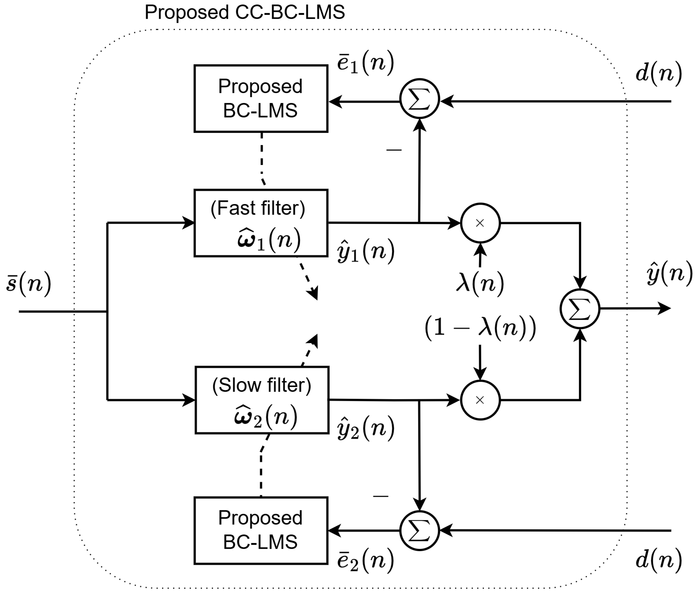
Figure 2 illustrates the block diagram of the proposed CC-BC-LMS method, which consists of two types of adaptive filter: one is the fast filter (with weight ω ^ 1 ( n ) and a larger step size μ 1 ) and the other is the slow filter (with weight ω ^ 2 ( n ) and a smaller step size μ 2 ). The output of the convex-combined filter is expressed as follows:
y ^ ( n ) = λ ( n ) y ^ 1 ( n ) + ( 1 λ ( n ) ) y ^ 2 ( n ) ,
where λ ( n ) [ 0 , 1 ] is the combination factor.
The combination parameter λ ( n ) is used to adjust the mixing ratio between the two sets of filter coefficients. It can be computed using the S-function (sigmoid function) as described in [29], as shown in Equation (15).
λ ( n + 1 ) = [ 1 + exp ( β ( n + 1 ) ) ] 1 .
The coefficient β ( n ) is updated by the following recursion:
β ( n + 1 ) = β ( n ) + δ β ( n ) ,
where sgn ( · ) denotes the sign function; δ β ( n ) = μ β sgn ( e ¯ ( n ) ) λ ( n ) 1 λ ( n ) y ^ 1 ( n ) y ^ 2 ( n ) and μ β is the learning rate used to update the weight β ( n ) . Note that a small value of μ β confers high stability but impairs tracking, leading to transient performance degradation following changes in the unknown system; in practice, λ ( n ) responds sluggishly, the handover from the fast to the slow branch is delayed, and the error curve decays smoothly yet slowly. Conversely, a large μ β induces rapid fluctuations in λ ( n ) , visible ripples in the learning curves, occasional mode switches under impulsive disturbances, and a risk of instability; while initial tracking is accelerated, the steady-state degrades through increased variance (higher NMSD and a heightened susceptibility to outliers. Following the approach in [30], we enforce the constraint | β ( n + 1 ) | β + and verify this condition every N 0 iterations. If β ( n + 1 ) falls below β + , we assign λ ( n + 1 ) = 0 ; conversely, if β ( n + 1 ) exceeds β + , we assign λ ( n + 1 ) = 1 .
In addition, considering that the convex combination scheme may be significantly affected by impulsive noise during the transition from the fast filter to the slow filter, we introduce the parameter λ C as a smoothed version of the combination parameter to improve the robustness of the algorithm as follows:
λ C ( n + 1 ) = 1 τ = n τ + 2 n + 1 λ ( ) ,
where τ determines the degree of smoothing of the combination parameter λ . Note that a practical way to set τ is to tie it to the time scales of two phenomena: how quickly λ should react to genuine changes, and how long impulsive disturbances last. The aim is to average out outliers without blurring true transitions between the fast and slow filters. A too-large τ leads to a noticeable lag during handovers (slow tracking after system changes), potential temporary performance loss right after changes, and risk of under-utilizing informative short-lived trends; on the contrary, a too-small τ is prone to high jitter in λ , greater sensitivity to outliers, possible oscillations in the combination weight, noisier transient and steady-state behavior, and it may overreact to impulsive noise, hurting NMSD.
The update recursion for each component filter ω ^ i ( n ) is as follows:
ω ^ i ( n + 1 ) = ω ^ i ( n ) + δ ω ^ i ( n ) + c i ( n )
with the correction term
δ ω ^ i ( n ) = μ i s ¯ ( n ) e ¯ i ( n )
with e ¯ i ( n ) = d ( n ) y ^ i ( n ) , and the bias compensation term c i ( n ) as follows:
c i ( n ) = μ i R ˜ η ( n ) ω ^ i ( n ) .
Thus, the resulting weight vector of the convex-combined system can be calculated below:
ω ^ ( n + 1 ) = λ C ( n + 1 ) ω ^ 1 ( n + 1 ) + ( 1 λ C ( n + 1 ) ) ω ^ 2 ( n + 1 ) .

3.3. Mean Stability Analysis

By substituting Equation (7) into Equation (4) and then taking the expectation on both sides, we have the following:
E ω ˘ ( n + 1 ) = E ω ˘ ( n ) + μ E e ¯ ( n ) s ¯ ( n ) + R ˜ η ( n ) ω ^ ( n ) .
In addition, the term E e ¯ ( n ) s ¯ ( n ) can be expressed as follows:
E e ¯ ( n ) s ¯ ( n ) = ( R s ( n ) E ω ˘ ( n ) + R η ( n ) E ω ^ ( n ) ) ,
where we denote the autocorrelation matrix of the noise-free input signal and input noise as R s ( n ) = E s ( n ) s T ( n ) and R η ( n ) = E η ( n ) η T ( n ) , respectively. Using Equation (23), we can rewrite Equation (22) as follows:
E ω ˘ ( n + 1 ) = [ I μ R s ( n ) ] E ω ˘ ( n ) + μ [ R ˜ η ( n ) R η ( n ) ] E ω ^ ( n ) .
If R ˜ η ( n ) R η ( n ) holds, we have
E ω ˘ ( n + 1 ) = [ I μ R s ( n ) ] E ω ˘ ( n ) .
Thus, the mean stability is derived as follows:
0 < μ < 2 λ max R s ( n ) ,
where λ max R s ( n ) denotes the maximum eigenvalue of the autocorrelation matrix of s ( n ) . Note that the convex combined architecture inclines to the component filter with a small step size [31]. Thus, the mean stability of the CC-BC-LMS algorithm is guaranteed if the inequality (26) holds.

3.4. Computational Complexity Analysis

Computational complexity is an important metric for evaluating the performance of an algorithm. To verify the practical feasibility of the proposed CC-BC-LMS algorithm, we analyze its computational complexity, emphasizing the arithmetic cost in terms of adders and multipliers. Table 1 presents the computational complexity of the proposed algorithm at different stages, including filter output, error signal, gradient update vector, weight update vector, bias compensation vector, and combined weight update vector for both fast and slow filters.
As shown in Table 1, the proposed algorithm requires a total of ( 8 K + 1 ) additions and ( 10 K + 6 ) multiplications. Furthermore, Table 2 compares the computational complexity of the proposed algorithm with other existing algorithms. Although the proposed method exhibits a higher computational cost, it significantly improves the tracking performance of bias-compensated algorithms by employing a threshold-based decision scheme for the convex combination parameter. Moreover, the convex combination approach achieves the effect of a variable step size, resulting in faster convergence and lower steady-state error. The trade-off of increased complexity leads to enhanced algorithmic performance.

4. Simulation Results

The impulse responses of the unknown system are Gaussian distributed with length K = 32 , which also sets the adaptive filter length and the K used in Section 3.4’s complexity counts. To assess the tracking performance of the adaptive filtering algorithms, the unknown system response ω was abruptly changed to ω at n = 2.5 × 10 5 , which corresponds to the midpoint of the simulation. In this work, we utilize two standard approaches to represent impulse noise. We begin with the BG model [33], which can be formulated as follows:
ζ ( n ) = b ( n ) · v ζ ( n ) ,
where b ( n ) follows a Bernoulli distribution with P ( b ( n ) = 1 ) = p and P ( b ( n ) = 0 ) + P ( b ( n ) = 1 ) = 1 . The term v ζ ( n ) corresponds to a zero-mean white Gaussian noise process with variance σ ζ 2 . The alpha-stable impulse noise model [34] is adopted as the second methodology and is specified by the parameter vector V s = ( s , s , s , s ) . In this parameterization, 0 < s < 2 denotes the characteristic exponent, s the skewness, s the dispersion, and s the location; notably, a smaller s yields stronger impulsive behavior.
To assess algorithm performance under temporally correlated input noise, the original white Gaussian input is replaced with a first-order autoregressive (AR1) process. Specifically, a zero-mean Gaussian process with unit variance is passed through the transfer function H 1 ( z ) to generate the AR1 input noise signal, as given by
H 1 ( z ) = 1 1 + b 1 z 1 ,
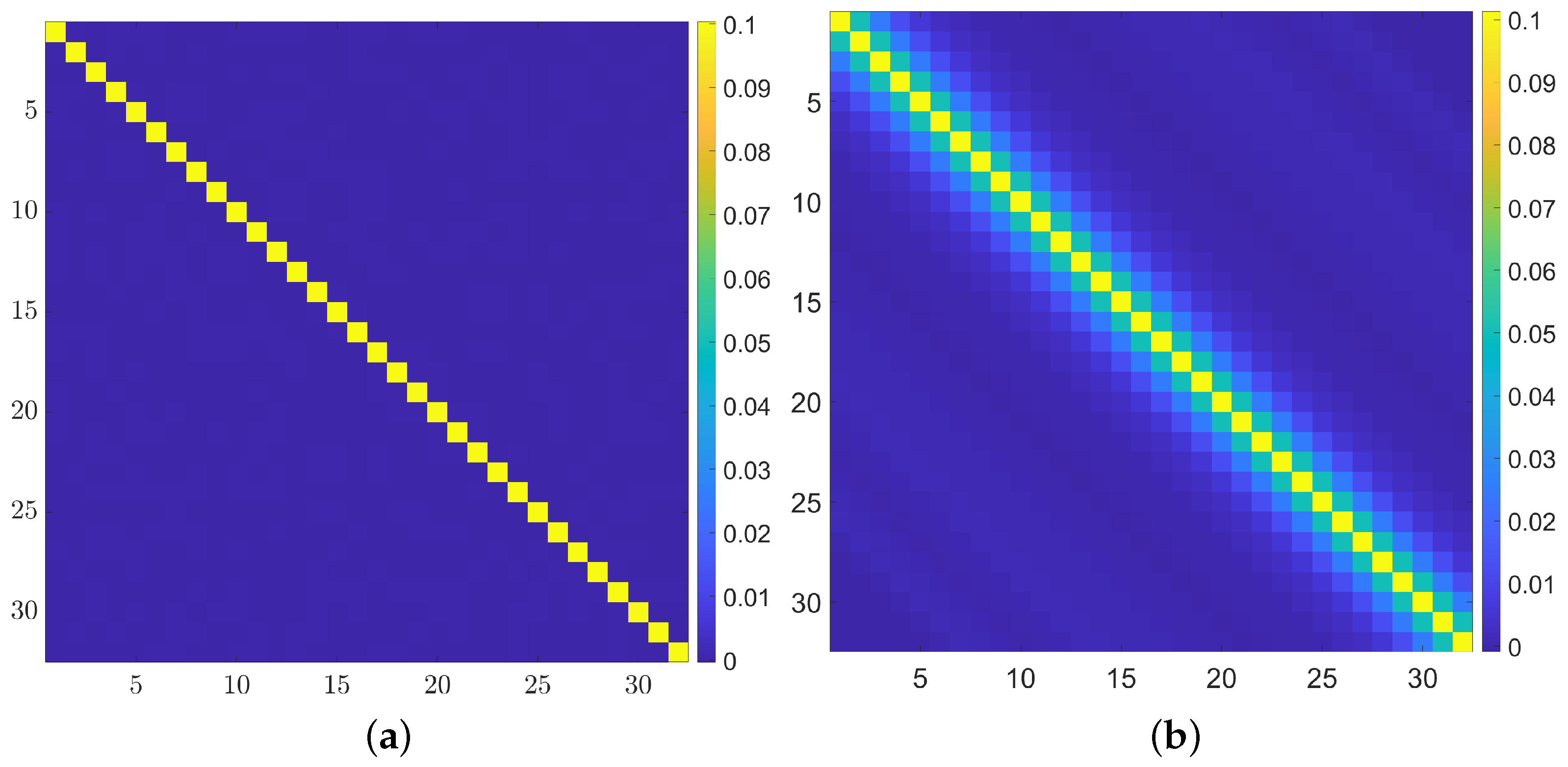
where b 1 = 0.5 . The resulting sample autocorrelation matrices for AWGN and AR(1) signals are illustrated in Figure 3. As expected, the matrix is almost perfectly diagonal because discrete-time white noise has zero correlation at all nonzero lags and a spike at lag 0; in contrast, the bright band widens around the diagonal and decays as distance from the diagonal increases, reflecting the AR(1) property, i.e., near-diagonal elements are high because adjacent samples are correlated, and values decrease geometrically for larger separations.
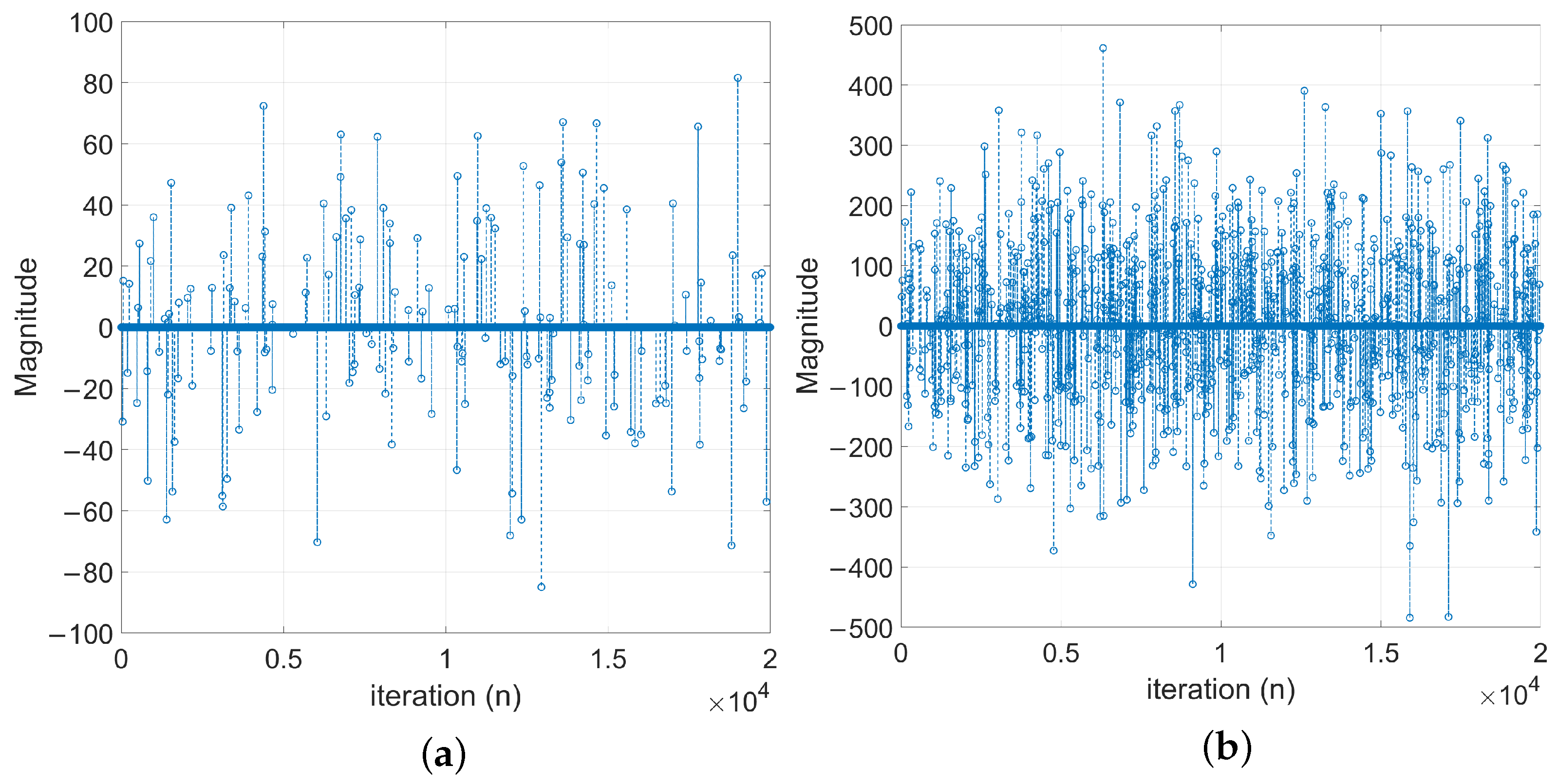
We consider the inputs to be standard white Gaussian distributed in the simulations. The additive input noise is set at SNR η = 10 dB; the measurement noise of ν ( n ) is set at SNR v = 30 dB. The simulated BG impulsive noise is divided into two signal strengths based on the probability of event occurrence: (1) mild impulsive noise ( p = 0.01 , SNR ζ = 15 dB ); (2) strong impulsive noise ( p = 0.05 , SNR ζ = 30 dB ). The illustrative traces are shown in Figure 4.
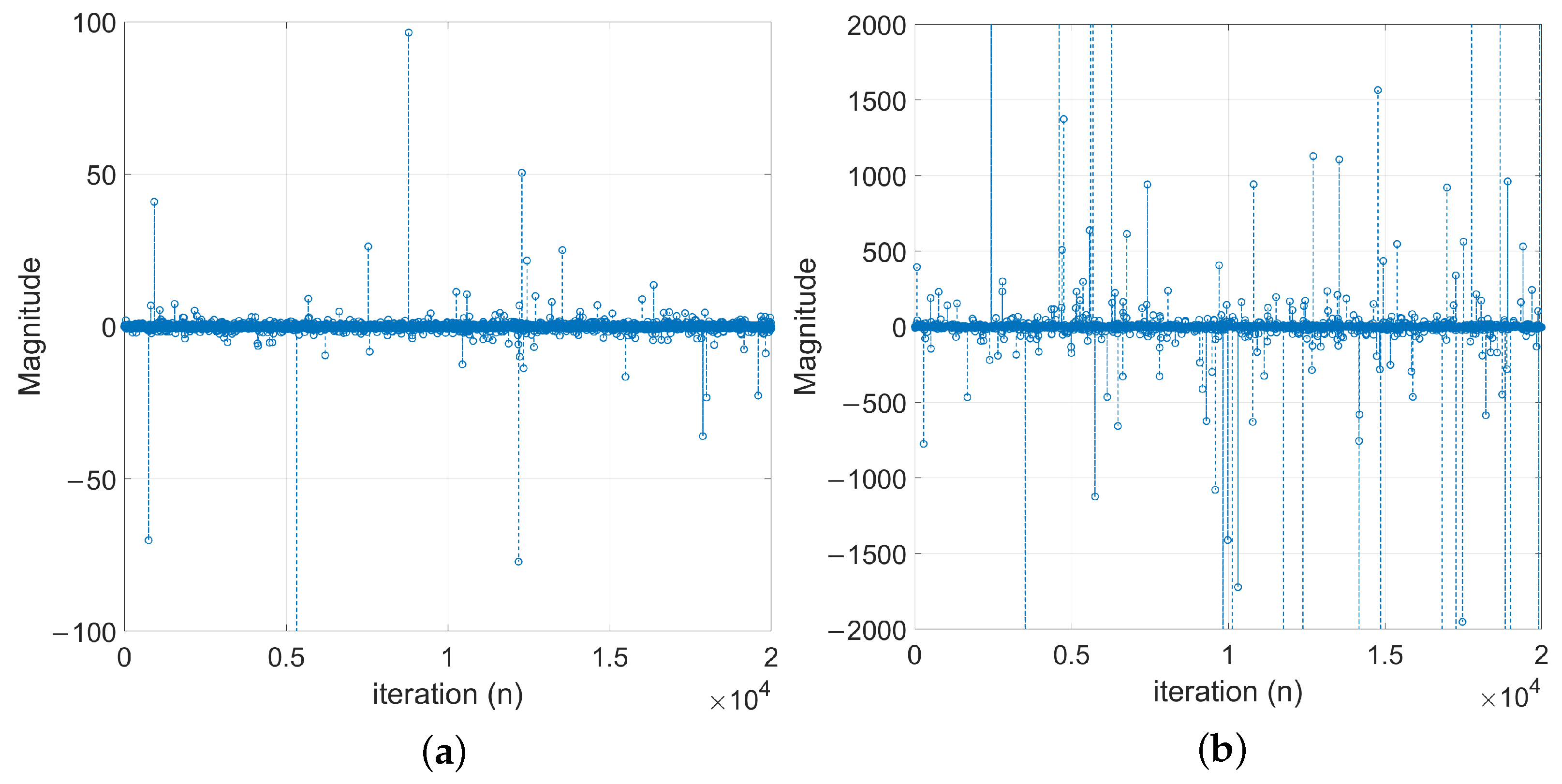
For α -stable impulsive noise, the signals are classified into two levels of intensity based on the characteristic exponent α s : (1) mild impulsive noise with V s = ( 1.4 , 0 , 0.1 , 0 ) ; (2) strong impulsive noise with V s = ( 0.7 , 0 , 0.1 , 0 ) . The illustrative traces are shown in Figure 5.
Regarding the evaluation of algorithm performance, we adopt the normalized mean square deviation (NMSD), whose mathematical definition is given in Equation (29), with units in decibels (dB):
NMSD ( n ) = 10 log 10 | | ω ω ^ ( n ) | | 2 2 | | ω | | 2 2 .
To ensure a fair comparison, we select the appropriate step sizes for each algorithm so that all algorithms exhibit similar convergence speeds. The detailed parameters for each algorithm are shown in Table 3. The other main parameter settings used in this paper are as follows: τ = 10 3 , β + = 8 , μ β = 10 , and N 0 = 1 . Unless otherwise stated, each reported curve is the average over 100 independent Monte Carlo trials, where independence spans both inputs and noise realizations; for BG we resample the Bernoulli events and Gaussian amplitudes each trial; for α -stable, we resample i.i.d. draws per trial; and for colored input noise we regenerate ν ( n ) via the AR(1) model each trial.

4.1. Evaluation of Robust Estimation of R ˜ η ( n )

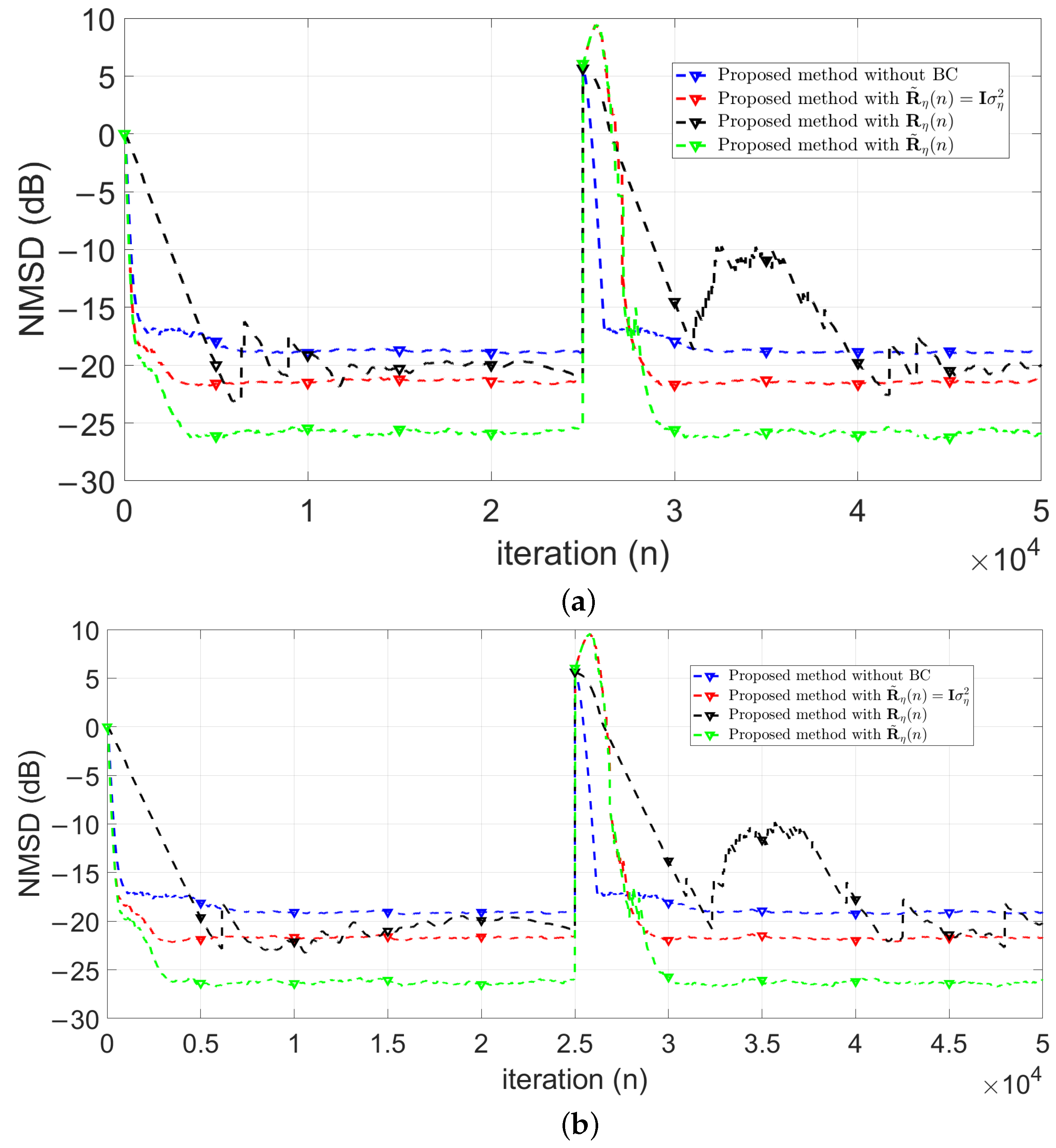
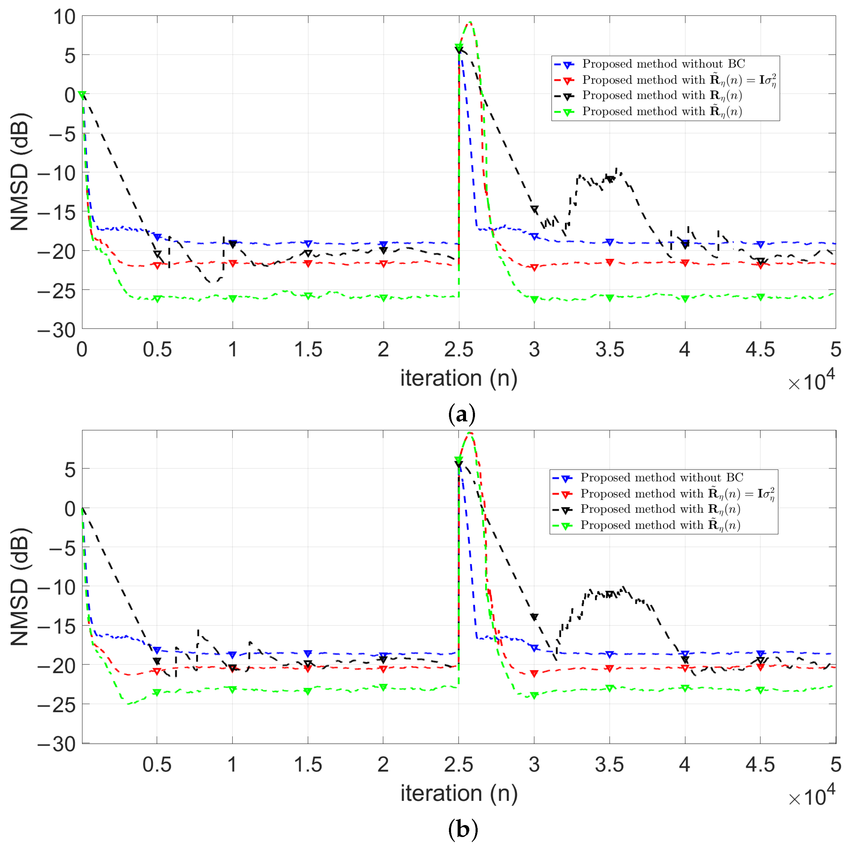
To evaluate the effectiveness of Equation (13), we consider four cases: No bias compensation (proposed method without BC); R ˜ η ( n ) = I σ η 2 (proposed method); R ˜ η ( n ) = E η η T (proposed method with R η ); and R ˜ η ( n ) in Equation (13) (proposed method with R ˜ η ( n ) ).
Figure 6a illustrates the case of mild BG impulses. In steady state, the curve with compensation differs from the one without compensation by 2.53 dB. Furthermore, using the autocorrelation matrix R ˜ η for compensation improves the compensated curve by an additional 4.43 dB. Figure 6b shows the case of strong BG impulses. In this scenario, the curve with compensation differs from the one without compensation by 2.55 dB in the steady state, and the use of the autocorrelation matrix R ˜ η for compensation further enhances the compensated curve by 5.01 dB.
Figure 7a examines the scenario of mild alpha-stable impulses. In steady state, the difference between the curve with compensation and the one without compensation is 2.46 dB. Additionally, employing the autocorrelation matrix R ˜ η for compensation further improves the compensated curve by 4.33 dB. Figure 7b illustrates the case of strong alpha-stable impulses. In this situation, the steady-state difference between the compensation curve and the one without compensation is 1.75 dB, and applying the autocorrelation matrix R ˜ η for compensation results in an additional improvement of 2.44 dB.
Based on observations from simulation results, it can be seen that simply using the autocorrelation matrix R η does not produce satisfactory performance. However, applying our proposed method with the autocorrelation matrix R ˜ η achieves significantly lower NMSD values in environments where input noise exhibits temporal correlation, compared to methods that do not account for colored input noise. This demonstrates the effectiveness of the R ˜ η approach.

4.2. Comparisons with Related Works

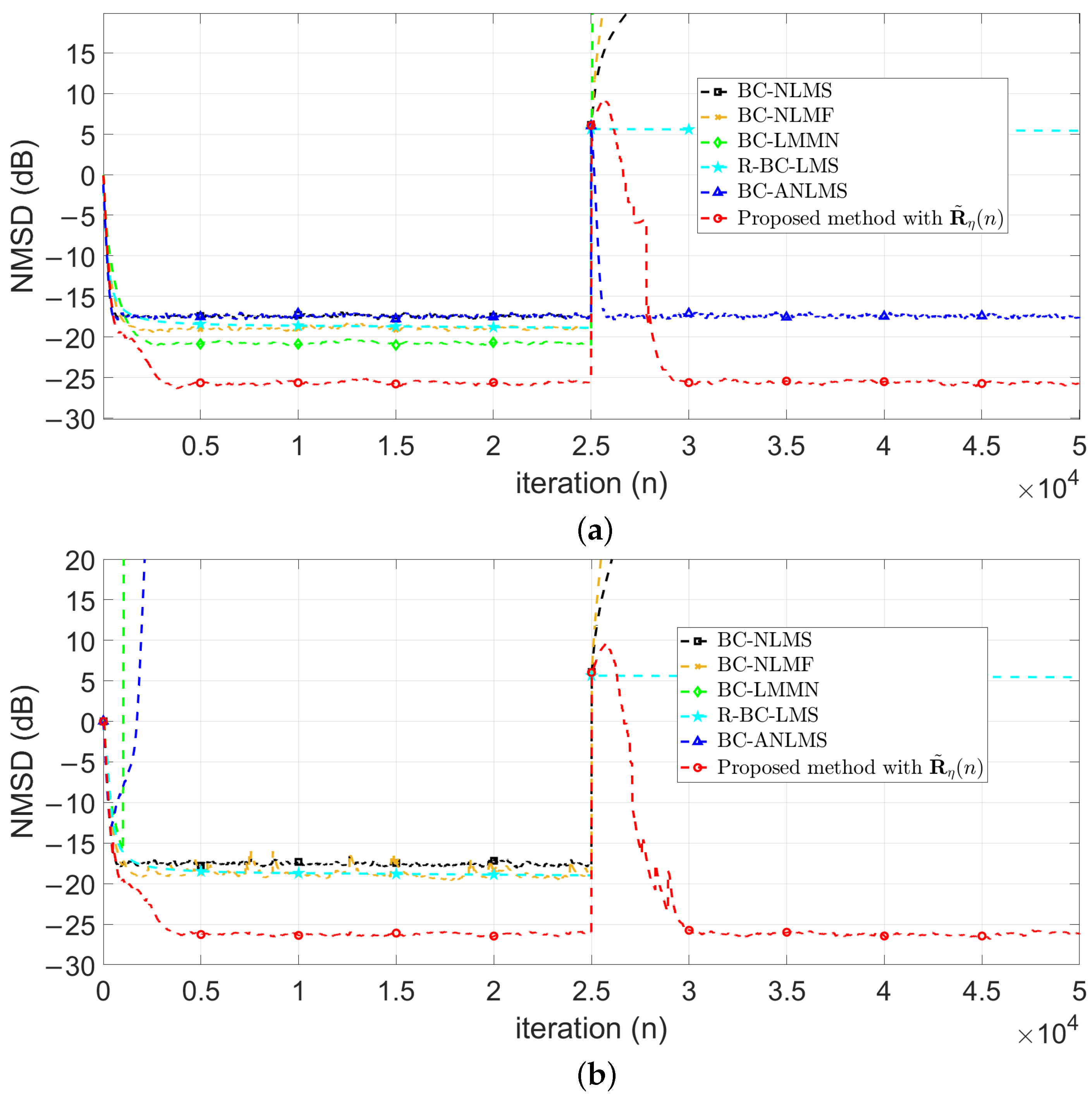
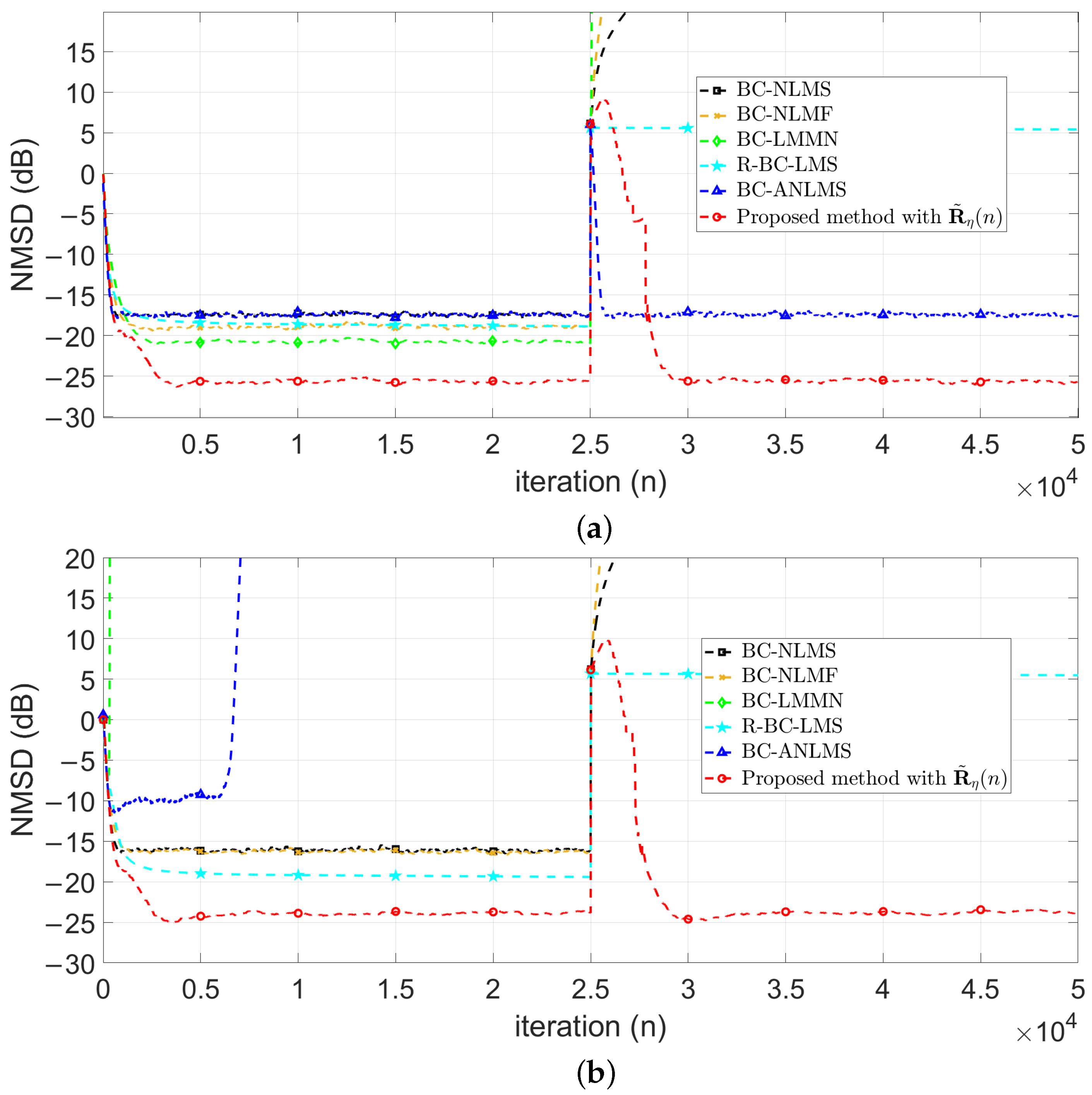
In Figure 8 and Figure 9, we simulate the performance of our proposed algorithm using the autocorrelation matrix R ˜ η under different intensities of BG impulses and alpha-stable impulses, comparing the NMSD curves with those of other algorithms. The duration of the simulation is n = 5 × 10 4 , and the channel change occurs at n = 2.5 × 10 4 . The step size parameters are consistent with those listed in Table 3.
Figure 8a shows the case of mild BG impulses. In steady state, our method outperforms other algorithms by 5.06 dB to 11.4 dB. Figure 8b illustrates the case of strong BG impulses, where our method achieves improvements of 7.45 dB to 11.17 dB compared to other algorithms. Table 4 summarizes the steady-state NMSD values (before the unknown system variation) for our proposed algorithm and other methods under different intensities of the BG impulses.
Figure 9a presents the case of mild α -stable impulses, where our method achieves improvements of 4.81 dB to 8.19 dB over other algorithms in the steady state. Figure 9b shows the case of strong α -stable impulses, where our method similarly outperforms others by 4.48 dB to 7.48 dB in the steady state. Table 5 lists the steady-state NMSD values (before the unknown variation of the system) for our proposed algorithm and other methods under different intensities of α -stable impulses.
While the proposed CC-BC-LMS increases multiplications due to the dual-branch convex combination and bias-compensation terms, its per-iteration arithmetic remains linear in filter length K and involves only vector multiply–accumulate (MAC) and simple elementwise operations, preserving LMS-class real-time viability on hardware implementation [35]. From the algorithm design perspective, the data selection scheme may possibly further reduce the unnecessary weight-updating, so that the computational cost may be lower [36]. In practice, hardware cost can be further reduced by look-up table (LUT) or piecewise-linear approximation of the sigmoid, fixed-point Huber thresholding, subsampling the bias-compensation update, or adopting partial/proportionate updates for large K [37], all with minimal impact on the demonstrated NMSD gains of 4.48 11.4 dB that motivate the added arithmetic in challenging colored/impulsive noise settings.

4.3. Evaluation of the Smoothed Convex-Combination

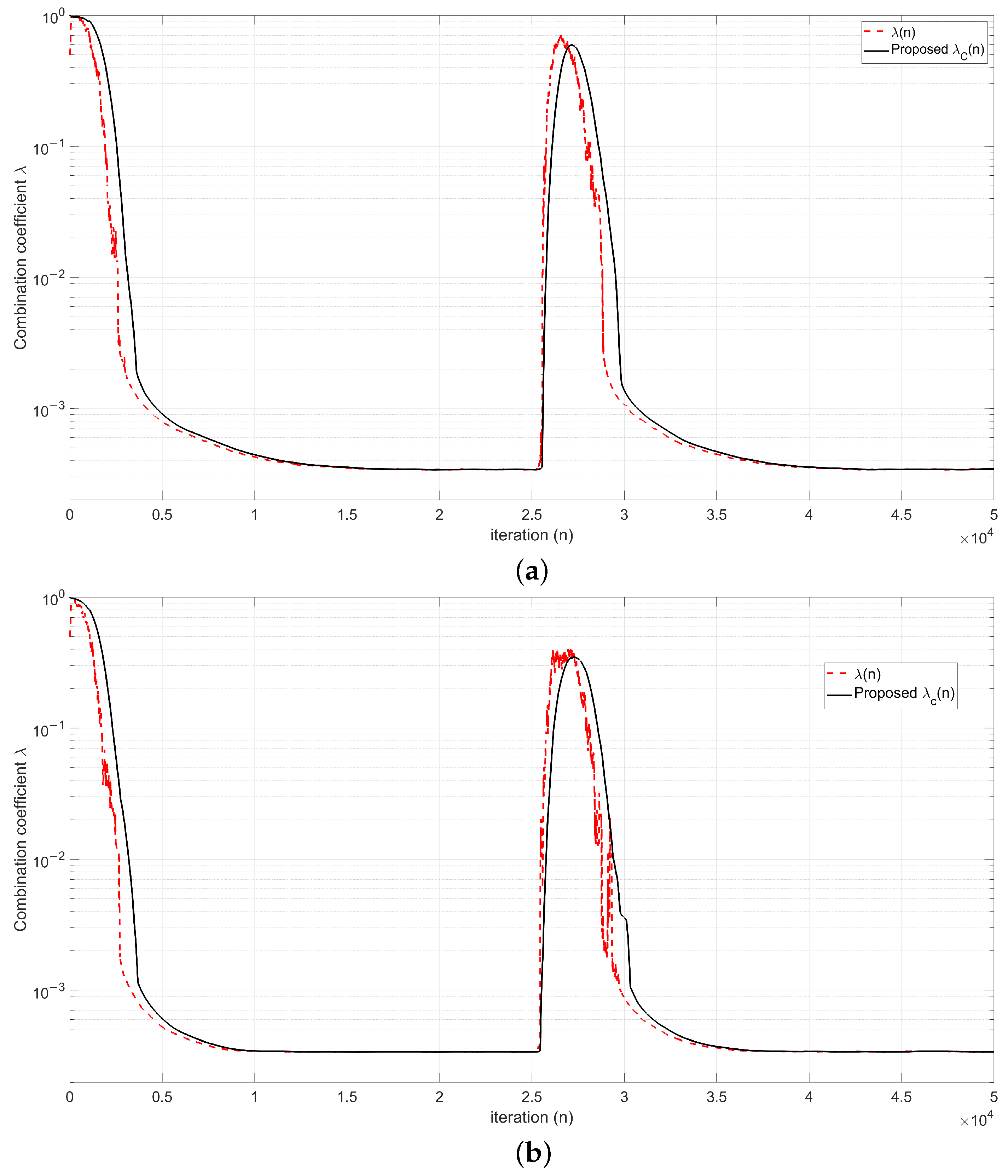
Figure 10 presents the learning curves of the combination coefficient for the two-component filter under different noise conditions. The simulation results demonstrate the following observations: (1) Without smoothing, the combination coefficients λ ( n ) exhibit pronounced fluctuations, particularly during the transient phases, that is, for n ( 0 , 0.5 ) ( 2.5 , 5 ) × 10 5 . (2) When strong impulse noise is present, as illustrated in Figure 10b, the transient regions exhibit more pronounced fluctuations than those observed under the mild impulse noise conditions depicted in Figure 10a. The proposed smoothing method effectively suppresses these variations, resulting in a more stable combination coefficient throughout the adaptation process.

5. Conclusions

This paper introduced a novel convex combination bias-compensated least mean square (CC-BC-LMS) algorithm, specifically designed to address the challenges of colored Gaussian input noise and impulsive observation noise in adaptive filtering. The proposed algorithm integrates bias compensation, robust error handling, and a variable step-size mechanism through a convex combination. The simulation results confirmed its superior performance compared to the existing methods.
The CC-BC-LMS algorithm effectively compensates for biases caused by colored Gaussian input noise by estimating and utilizing an autocorrelation matrix. Additionally, the use of the modified Huber function ensures robustness against impulsive observation noise, enabling reliable operation under both mild and strong impulse conditions. The convex combination approach dynamically adjusts between fast and slow filters, achieving faster convergence and reduced steady-state error.
Performance evaluations demonstrated that the proposed method consistently outperforms the state-of-the-art algorithms in terms of NMSD, with improvements ranging from 4.48 dB to 11.4 dB under various noise conditions. Although the algorithm incurs higher computational complexity, this trade-off is justified by its enhanced robustness and improved convergence behavior.

Author Contributions

Conceptualization, Y.-R.C., H.-E.H. and G.Q.; methodology, Y.-R.C. and H.-E.H.; software, Y.-R.C. and H.-E.H.; validation, Y.-R.C. and G.Q.; formal analysis, Y.-R.C. and H.-E.H.; investigation, H.-E.H.; resources, Y.-R.C. and H.-E.H.; data curation, Y.-R.C. and H.-E.H.; supervision, Y.-R.C.; writing—original draft preparation, Y.-R.C. and H.-E.H.; writing—review and editing, Y.-R.C., H.-E.H. and G.Q.; project administration, Y.-R.C.; funding acquisition, Y.-R.C. All authors have read and agreed to the published version of the manuscript.

Funding

This work was supported in part by the National Science and Technology Council (NSTC), Taiwan, under Grant 113-2221-E-027-130.

Data Availability Statement

The original contributions presented in this study are included in the article. Further inquiries can be directed to the corresponding author.

Conflicts of Interest

The authors declare no conflicts of interest.

Abbreviations

The following abbreviations are used in this manuscript:
AR(1)First-Order Autoregressive Process
BCBias Compensation
BC-ANLMSBias-Compensated Arctangent NLMS
BC-LMMNBias-Compensated Least Mean Mixed-Norm
BC-NLMFBias-Compensated Normalized Least Mean Square
BCE-NLMSBias-Compensated Error-Modified NLMS
BGBernoulli-Gaussian
CC-BC-LMSConvex Combination Bias-Compensated LMS
DOADirection of Arrival
EIVErrors-In-Variable
FIRFinite Impulse Response
LMSLeast Mean Square
MAPMaximum A Posteriori
NLMSNormalized Least Mean Square
NLMFNormalized Least Mean Fourth
MMCCMixture Maximum Correntropy Criterion
NMSDNormalized Mean Square Deviation
PDFProbability Density Function
R-BC-LMSRobust Bias-Compensated LMS
SNRSignal-to-Noise Ratio
α -stableSymmetric Alpha-Stable Distribution

References

  1. Söderström, T. Errors-in-variables methods in system identification. Automatica 2007, 43, 939–958. [Google Scholar] [CrossRef]
  2. Dang, L.; Wang, W.; Chen, B. Square Root Unscented Kalman Filter With Modified Measurement for Dynamic State Estimation of Power Systems. IEEE Trans. Instrum. Meas 2022, 71, 9002213. [Google Scholar] [CrossRef]
  3. Dang, L.; Yang, J.; Liu, M.; Chen, B. Differential Equation-Informed Neural Networks for State-of-Charge Estimation. IEEE Trans. Instrum. Meas 2024, 73, 1000315. [Google Scholar] [CrossRef]
  4. Schaffrin, B. Total Least-Squares Collocation: An Optimal Estimation Technique for the EIV-Model with Prior Information. Mathematics 2020, 8, 971. [Google Scholar] [CrossRef]
  5. Dang, L.; Huang, Y.; Zhang, Y.; Chen, B. Multi-kernel correntropy based extended Kalman filtering for state-of-charge estimation. ISA Trans. 2022, 129, 271–283. [Google Scholar] [CrossRef]
  6. Yao, Y.; Guo, T.N.; Chen, Z.; Fu, C. A Fast Multi-Source Sound DOA Estimator Considering Colored Noise in Circular Array. IEEE Sens. J. 2019, 19, 6914–6926. [Google Scholar] [CrossRef]
  7. Amato, G.; D’Amato, R.; Ruggiero, A. Adaptive Rejection of a Sinusoidal Disturbance with Unknown Frequency in a Flexible Rotor with Lubricated Journal Bearings. Mathematics 2022, 10, 1703. [Google Scholar] [CrossRef]
  8. Zhou, Y.; Zhao, H.; Liu, D.; Guo, X. Distributed Active Noise Control Robust to Impulsive Interference. IEEE Sens. J. 2025, 25, 11480–11490. [Google Scholar] [CrossRef]
  9. Wang, H.; Ma, J.; Huang, Z.; Liu, K. Multitarget Vital Signs Estimation Based on Millimeter-Wave Radar in Complex Scenes. IEEE Sens. J. 2024, 24, 39432–39442. [Google Scholar] [CrossRef]
  10. Abdelrhman, O.M.; Lv, S.; Li, S.; Dou, Y. Modified Sigmoid Function-Based Proportionate Diffusion Recursive Adaptive Filtering Algorithm Over Sensor Network. IEEE Sens. J. 2024, 24, 39478–39489. [Google Scholar] [CrossRef]
  11. Hou, X.; Zhao, H.; Long, X. Robust Linear-in-the-Parameters Nonlinear Graph Diffusion Adaptive Filter Over Sensor Network. IEEE Sens. J. 2024, 24, 16710–16720. [Google Scholar] [CrossRef]
  12. Sharma, P.; Mohan Pradhan, P. Modeling Behavior of Sensors Using a Novel β-Divergence-Based Adaptive Filter. IEEE Sens. J. 2024, 24, 32641–32650. [Google Scholar] [CrossRef]
  13. Liu, C.; Zhao, H. Efficient DOA Estimation Method Using Bias-Compensated Adaptive Filtering. IEEE Trans. Veh. Technol. 2020, 69, 13087–13097. [Google Scholar] [CrossRef]
  14. Li, C.; Zhao, H.; Xiang, W. Bias-compensated based diffusion affine projection like maximum correntropy algorithm. Digit. Signal Process. 2024, 154, 104702. [Google Scholar] [CrossRef]
  15. Eweda, E. Global Stabilization of the Least Mean Fourth Algorithm. IEEE Trans. Signal Process. 2012, 60, 1473–1477. [Google Scholar] [CrossRef]
  16. Lee, M.; Park, T.; Park, P. Bias-Compensated Normalized Least Mean Fourth Algorithm for Adaptive Filtering of Impulsive Measurement Noises and Noisy Inputs. In Proceedings of the 2019 12th Asian Control Conference (ASCC), Kitakyushu, Japan, 9–12 June 2019; pp. 220–223. [Google Scholar]
  17. Chien, Y.R.; Hsieh, H.E.; Qian, G. Robust Bias Compensation Method for Sparse Normalized Quasi-Newton Least-Mean with Variable Mixing-Norm Adaptive Filtering. Mathematics 2024, 12, 1310. [Google Scholar] [CrossRef]
  18. Huang, F.; Song, F.; Zhang, S.; So, H.C.; Yang, J. Robust Bias-Compensated LMS Algorithm: Design, Performance Analysis and Applications. IEEE Trans. Veh. Technol. 2023, 72, 13214–13228. [Google Scholar] [CrossRef]
  19. Jung, S.M.; Park, P. Normalised least-mean-square algorithm for adaptive filtering of impulsive measurement noises and noisy inputs. Electron. Lett. 2013, 49, 1270–1272. [Google Scholar] [CrossRef]
  20. Yoo, J.; Shin, J.; Park, P. An Improved NLMS Algorithm in Sparse Systems Against Noisy Input Signals. IEEE Trans. Circuits Syst. Ii Exp. Briefs 2015, 62, 271–275. [Google Scholar] [CrossRef]
  21. Jin, Z.; Guo, L.; Li, Y. The Bias-Compensated Proportionate NLMS Algorithm With Sparse Penalty Constraint. IEEE Access 2020, 8, 4954–4962. [Google Scholar] [CrossRef]
  22. Jin, Z.; Yang, Z.; Li, Q.; Ma, L. Bias-Compensated PNLMS Algorithm With Multi-Segment Function for Noisy Input. IEEE Access 2025, 13, 43741–43748. [Google Scholar] [CrossRef]
  23. Wen, P.; Wang, B.; Qu, B.; Zhang, S.; Zhao, H.; Liang, J. Robust Bias-Compensated CR-NSAF Algorithm: Design and Performance Analysis. IEEE Trans. Syst., Man Cybern. Syst. 2025, 55, 674–684. [Google Scholar] [CrossRef]
  24. Long, X.; Zhao, H.; Hou, X. A Bias-Compensated NMMCC Algorithm Against Noisy Input and Non-Gaussian Interference. IEEE Trans. Circuits Syst. Ii Exp. Briefs 2023, 70, 3689–3693. [Google Scholar] [CrossRef]
  25. Rosalin, P.A.; Nanda, S. A bias-compensated NLMS algorithm based on arctangent framework for system identification. Signal Image Video Process. 2024, 18, 3595–3601. [Google Scholar] [CrossRef]
  26. So, H. LMS-based algorithm for unbiased FIR filtering with noisy measurements. Electron. Lett. 2001, 37, 1418–1420. [Google Scholar] [CrossRef]
  27. Zhao, H.; Zheng, Z. Bias-compensated affine-projection-like algorithms with noisy input. Electron. Lett. 2016, 52, 712–714. [Google Scholar] [CrossRef]
  28. Zhou, Y.; Chan, S.C.; Ho, K.L. New Sequential Partial-Update Least Mean M-Estimate Algorithms for Robust Adaptive System Identification in Impulsive Noise. IEEE Trans. Ind. Electron. 2011, 58, 4455–4470. [Google Scholar] [CrossRef]
  29. Arenas-Garcia, J.; Figueiras-Vidal, A.; Sayed, A. Mean-square performance of a convex combination of two adaptive filters. IEEE Trans. Signal Process. 2006, 54, 1078–1090. [Google Scholar] [CrossRef]
  30. Lu, L.; Zhao, H.; Li, K.; Chen, B. A Novel Normalized Sign Algorithm for System Identification Under Impulsive Noise Interference. Circuits Syst. Signal Process. 2015, 35, 3244–3265. [Google Scholar] [CrossRef]
  31. Arenas-Garcia, J.; Azpicueta-Ruiz, L.A.; Silva, M.T.; Nascimento, V.H.; Sayed, A.H. Combinations of Adaptive Filters: Performance and convergence properties. IEEE Signal Process. Mag. 2016, 33, 120–140. [Google Scholar] [CrossRef]
  32. Lee, M.; Park, I.S.; Park, C.E.; Lee, H.; Park, P. Bias Compensated Least Mean Mixed-norm Adaptive Filtering Algorithm Robust to Impulsive Noises. In Proceedings of the 2020 20th International Conference on Control, Automation and Systems (ICCAS), Busan, Republic of Korea, 13–16 October 2020; pp. 652–657. [Google Scholar] [CrossRef]
  33. Kim, S.R.; Efron, A. Adaptive robust impulse noise filtering. IEEE Transa. Signal Process. 1995, 43, 1855–1866. [Google Scholar] [CrossRef]
  34. Shao, M.; Nikias, C. Signal processing with fractional lower order moments: Stable processes and their applications. Proc. IEEE 1993, 81, 986–1010. [Google Scholar] [CrossRef]
  35. Thannoon, H.H.; Hashim, I.A. Hardware Implementation of a High-Speed Adaptive Filter Using a Combination of Systolic and Convex Architectures. Circuits Syst. Signal Process. 2024, 43, 1773–1791. [Google Scholar] [CrossRef]
  36. Chien, Y.R.; Wu, S.T.; Tsao, H.W.; Diniz, P.S.R. Correntropy-Based Data Selective Adaptive Filtering. IEEE Trans. Circuits Syst. I Regul. Pap. 2024, 71, 754–766. [Google Scholar] [CrossRef]
  37. Chien, Y.R.; Chu, S.I. A Fast Converging Partial Update LMS Algorithm with Random Combining Strategy. Circuits Syst. Signal Process. 2014, 33, 1883–1898. [Google Scholar] [CrossRef]
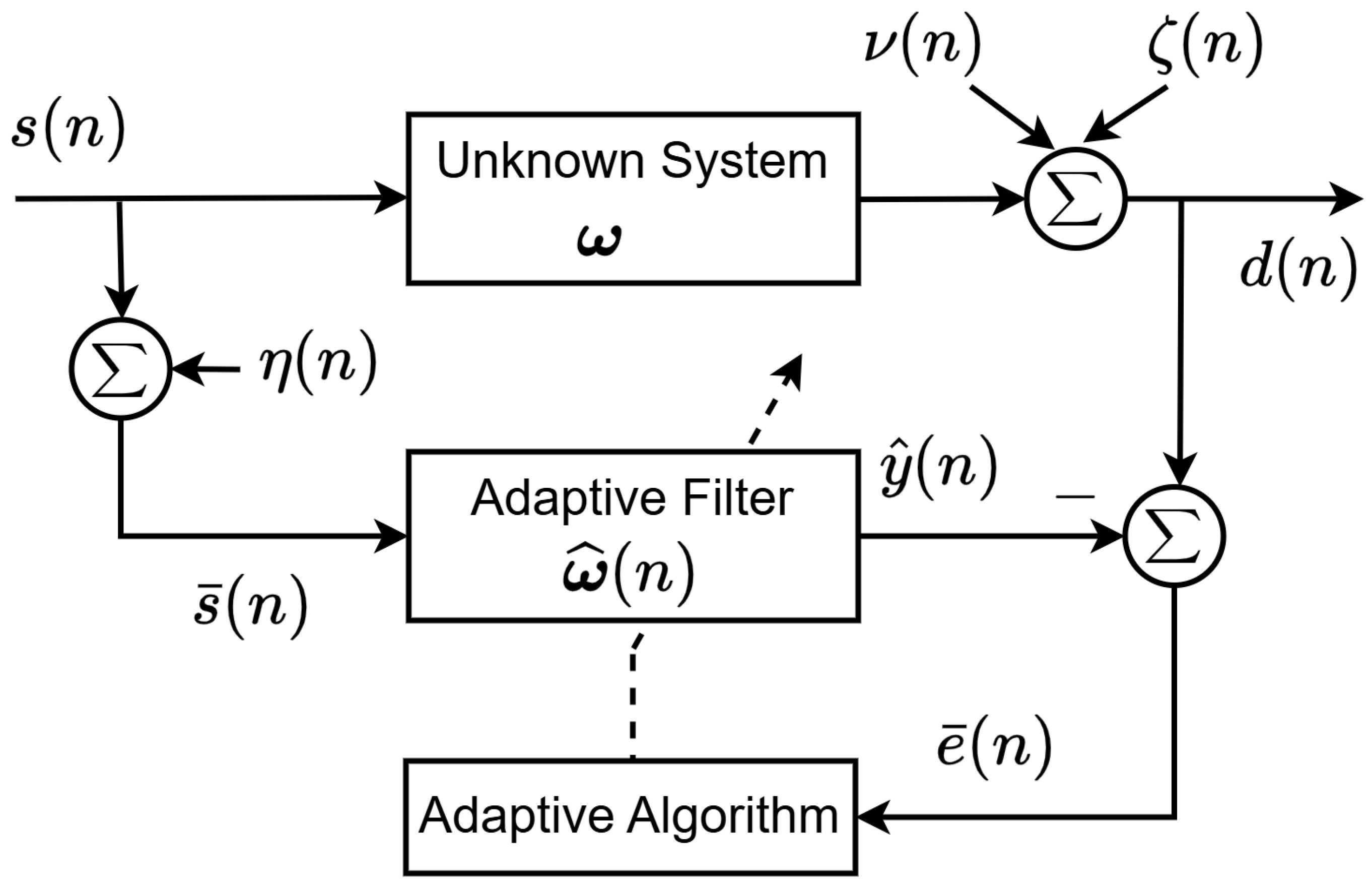
Figure 1. System model.
Mathematics 13 03348 g001
Figure 2. VSS approach by using convex combination technique.
Mathematics 13 03348 g002
Figure 3. Comparison of sample autocorrelation matrices over 32 lags: (a) AWGN and (b) AR(1).
Mathematics 13 03348 g003
Figure 4. Illustrative traces of BG impulse noise: (a) mild and (b) strong.
Mathematics 13 03348 g004
Figure 5. Illustrative traces of α -stable impulsive noise: (a) mild and (b) strong.
Mathematics 13 03348 g005
Figure 6. NMSD curves of the autocorrelation matrix R ˜ η for different BG impulse intensities: (a) mild and (b) strong impulses.
Mathematics 13 03348 g006
Figure 7. NMSD curves of the autocorrelation matrix R ˜ η for different α -stable impulse intensities: (a) mild and (b) strong impulses.
Mathematics 13 03348 g007
Figure 8. Comparison of NMSD curves for different intensities of BG impulses using the autocorrelation matrix R ˜ η and other algorithms: (a) mild and (b) strong impulses.
Mathematics 13 03348 g008
Figure 9. Comparison of NMSD curves for different intensities of α -stable impulses using the autocorrelation matrix R ˜ η and other algorithms: (a) mild and (b) strong impulses.
Mathematics 13 03348 g009
Figure 10. Comparison of learning curves for the combination factor under different intensities of α -stable impulses: (a) mild and (b) strong impulses.
Mathematics 13 03348 g010
Table 1. Computational complexity analysis of the proposed algorithm. All arithmetic counts are expressed as functions of the filter length K, which is identical to the FIR system length used in the simulations of Section 4.
No.CalculationsAdderMultiplier
1 y ^ i ( n ) = ω ^ i T ( n ) s ¯ i ( n ) K 1 K
2 e ¯ i ( n ) = d ( n ) y ^ i ( n ) 1-
3 δ ω ^ i ( n ) in Equation (19) 4 K 4 K + 2
4 c i ( n ) in Equation (20)- 2 K + 4
5 ω ^ i ( n + 1 ) in Equation (18) 2 K K
6 ω ^ ( n + 1 ) in Equation (21) K + 1 2 K
Total 8 K + 1 10 K + 6
Table 2. Comparison of computational complexity for different algorithms. All arithmetic counts are expressed as functions of the filter length K, which is identical to the FIR system length used in the simulations of Section 4.
AlgorithmsAdderMultiplier
BC-NLMS [19] 2 K 4 K
BC-NLMF [16] 2 K 5 K
BC-LMMN [32] 3 K 5 K
R-BC-SA-LMS [18] 8 K + 3 9 K + 28
BC-ANLMS [25] 3 K + 3 5 K + 12
Proposed 8 K + 1 10 K + 6
Table 3. Step-size parameters of each algorithm.
AlgorithmsStep Size
BC-NLMS [19] μ = 0.2
BC-NLMF [16] μ = 0.4
BC-LMMN [32] μ = 5 × 10 4
BC-ANLMS [25] μ = 0.2 , γ = 5 × 10 4
Proposed μ 1 = 5 × 10 3 , μ 2 = 1 × 10 3
Table 4. Steady-state (before the unknown system variation) NMSD comparison under different intensities of BG impulses.
AlgorithmsMild BGStrong BG
BC-NLMS [19] 17.7  dB 17.68  dB
BC-NLMF [16] 19.03  dB 15.17  dB
BC-LMMN [32] 21.15  dB(divergenced)
R-BC-SA-LMS [18] 18.85  dB 18.89  dB
BC-ANLMS [25] 15.17  dB(divergenced)
Proposed method with R ˜ η 26.21  dB 26.34  dB
Table 5. Steady-state (before the unknown system variation) NMSD comparison under different intensities of alpha-stable impulses.
AlgorithmsMild Alpha StableStrong Alpha Stable
BC-NLMS [19] 17.51  dB 16.3  dB
BC-NLMF [16] 19.35  dB 16.6  dB
BC-LMMN [32] 20.88  dB(divergenced)
R-BC-SA-LMS [18] 18.78  dB 19.37  dB
BC-ANLMS [25] 17.5  dB(divergenced)
Proposed method with R ˜ η 25.69  dB 23.78  dB
Disclaimer/Publisher’s Note: The statements, opinions and data contained in all publications are solely those of the individual author(s) and contributor(s) and not of MDPI and/or the editor(s). MDPI and/or the editor(s) disclaim responsibility for any injury to people or property resulting from any ideas, methods, instructions or products referred to in the content.