Statistical Analysis of the Induced Ailamujia Lifetime Distribution with Engineering and Bidomedical Applications

Abstract

Accurate modeling of industrial and biomedical data is often challenging due to skewness, heavy tails, and complex variability, which traditional probability distributions fail to capture. To address this, we propose the Induced Ailamujia Lifetime Distribution (IALD), a flexible generalization of the Ailamujia distribution developed via an induced transformation. The IALD accommodates diverse dataset characteristics through a wide range of probability density and hazard rate shapes. Several key statistical properties are derived, including moments, reliability measures, quantile and generating functions, probability weighted moments, and entropy measures. Model parameters are estimated using six classical methods, with their performance assessed through simulation. The practical utility of the IALD is demonstrated using two real datasets from biomedical and industrial fields, where it consistently outperforms existing lifetime models. These results confirm the IALD as a powerful and promising tool for reliability, engineering, and biomedical data analysis.

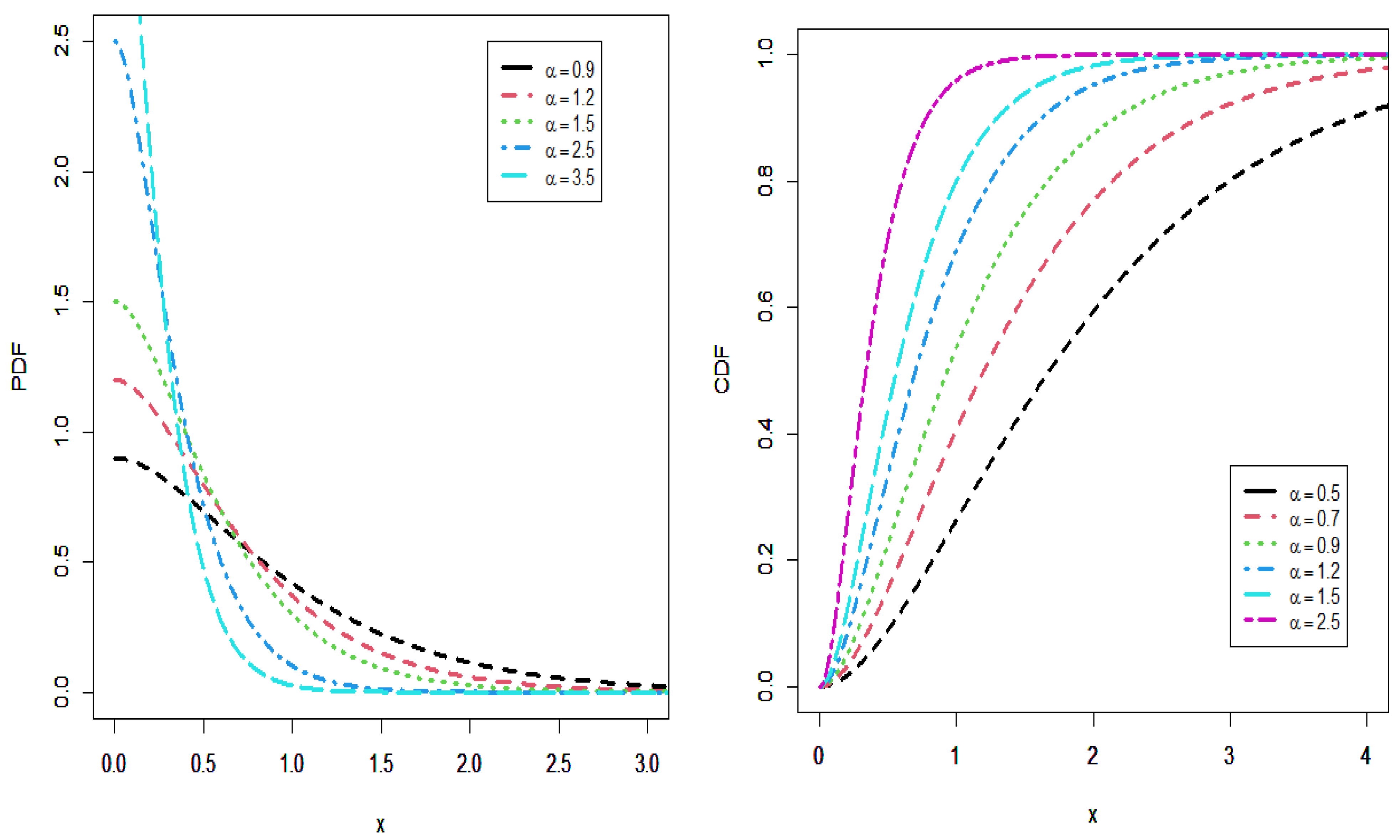
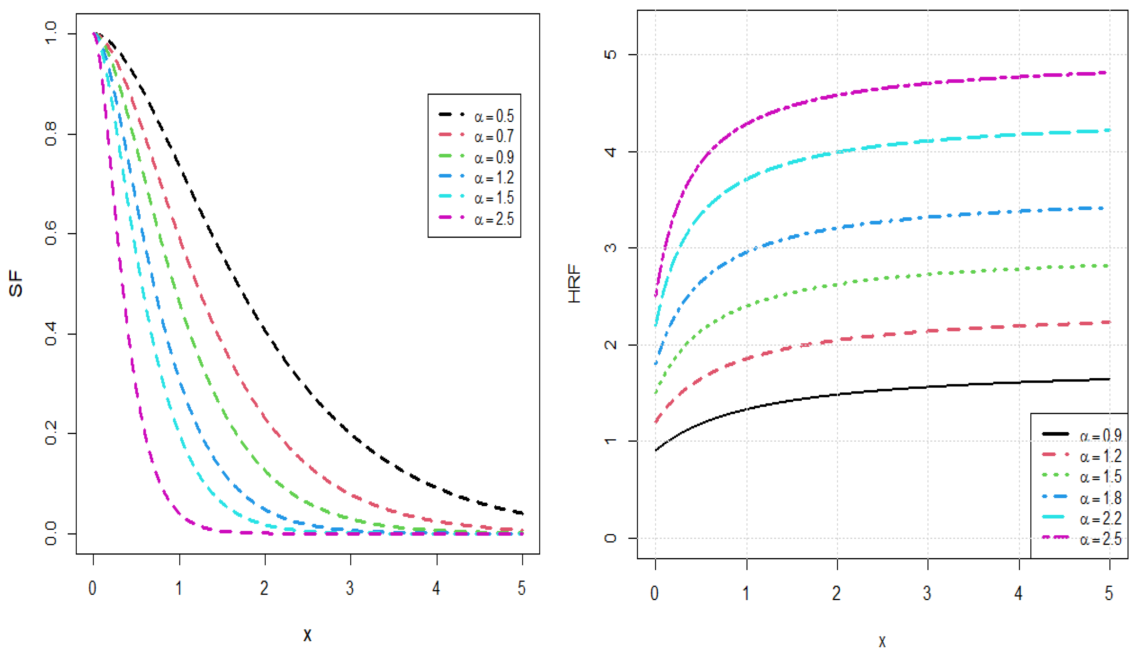
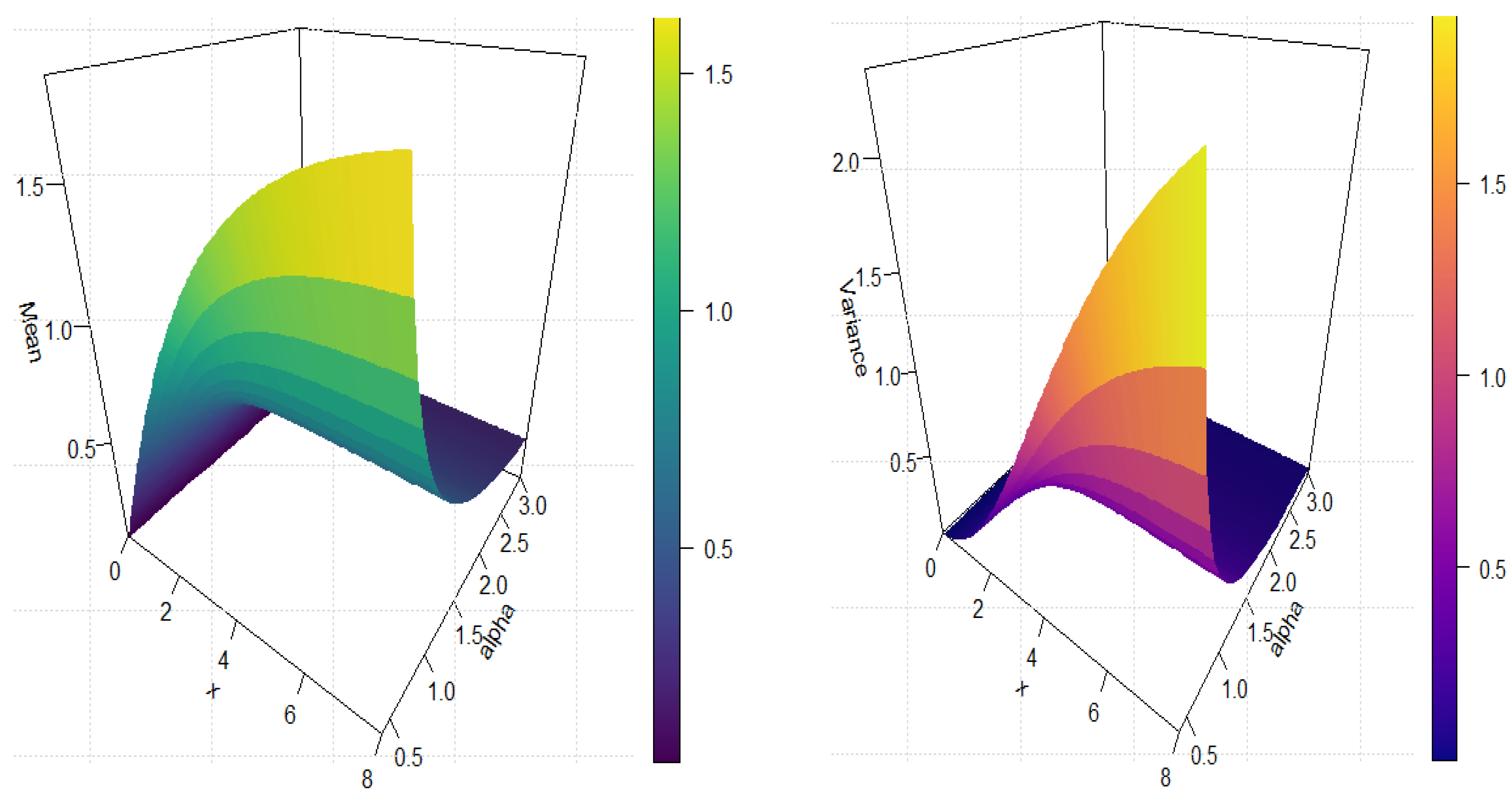
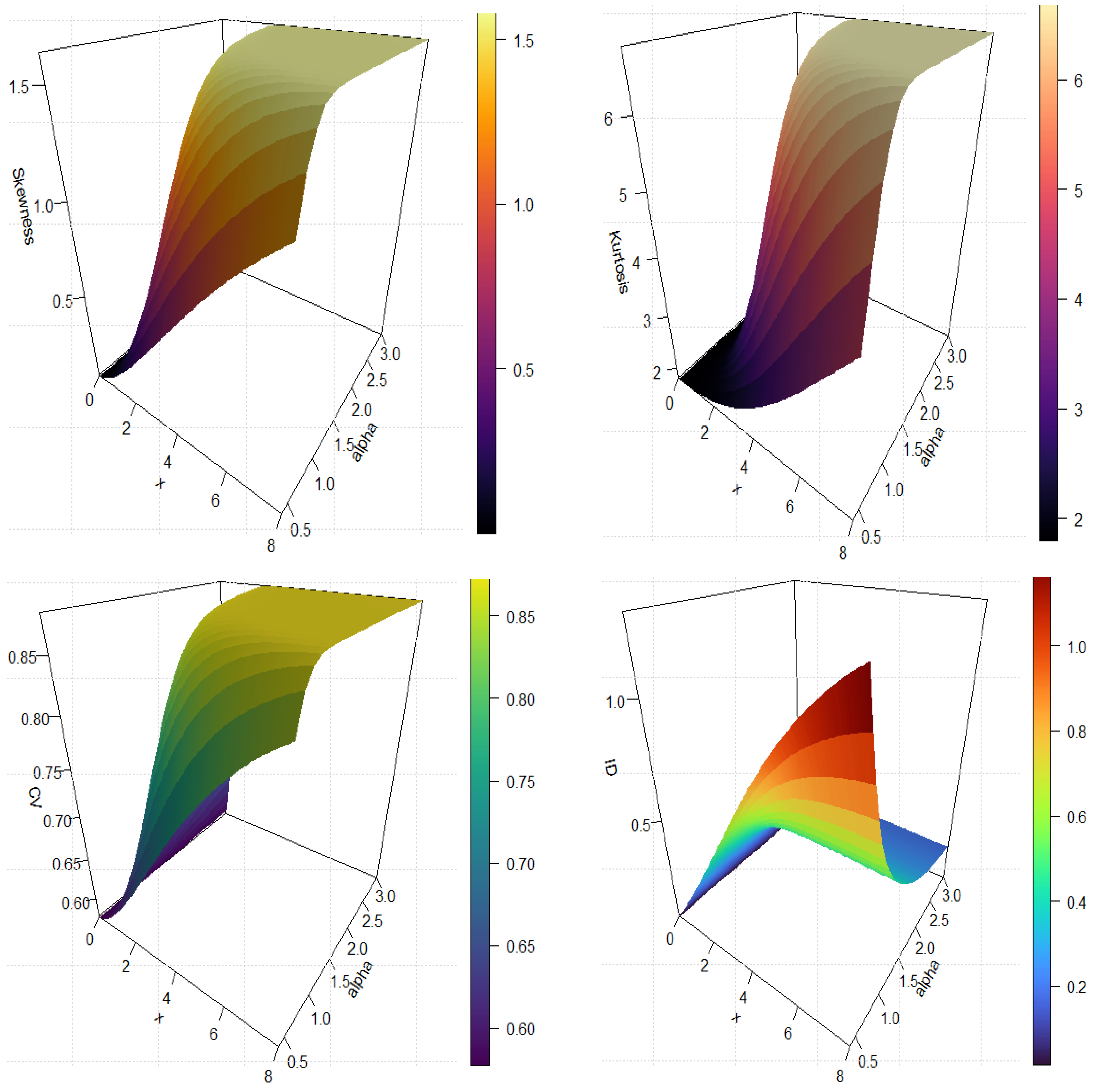
1. Introduction

Over the past century, numerous important probability distributions have been developed to serve as models across various scientific disciplines. In recent years, there has been growing interest in creating new classes of univariate continuous distributions to enhance the flexibility and applicability of existing ones. An established probability model can be extended through various approaches, leading to a wide array of new distributions. Statistical analysis and data modeling are essential in nearly all applied fields, including biomedical research, engineering, finance, demography, environmental sciences, and agriculture. The statistical literature offers a rich collection of continuous distributions for modeling lifetime data, such as the exponential, Lindley, beta, gamma, Weibull, Gompertz, lognormal, and normal distributions, among others. Several techniques are available for generalizing probability models, including the mixture and transformation of existing distributions, the transmutation method, non-parametric approaches, the power method, and the exponential method.

One notable approach to generating new probability distributions is through the concept of weighted distributions. In such models, weights are introduced to modify conventional probability calculations, allowing the probability of an event to be determined not merely by counting the number of data points but by summing the weights associated with those data points. This approach provides greater flexibility in modeling complex datasets, as individual observations can exert varying degrees of influence on the overall distribution. The idea of weighted distributions was first introduced by Fisher [1] and later extended by Patil and Rao [2]. Formally, let X be a random variable with probability density function (PDF) f(x), and suppose that the probability of observing X = x is proportional to a non-negative weight function $w(x) \ge 0$. Then, according to the weighted probability principle, the density function of the observed X is given by the following:

$$f_w(x) = {\displaystyle \frac{w\left(x) f\right(x)}{{\int }_{-\infty }^{\infty }w\left(x) f\right(x)\mathit{dx}}}.$$

The probability density function obtained from this formulation is referred to as the weighted density, and the function $\mathrm{w}\left(\mathrm{x}\right) \ge 0$ is called the weight function. The choice of $\mathrm{w}\left(\mathrm{x}\right)$ depends on the application, and various forms have been proposed in the literature. For instance, Mohiuddin et al. [3] introduced the weighted Nwikpe distribution using a linear weight function, while Hussain and Mohammed [4] applied an exponential-type weight in the weighted Zeghdoudi distribution. Ganaie and Rajagopalan [5] considered a length-biased form in the new quasi-Lindley model, whereas Alsmairan and Al-Omari [6] employed a quadratic-type weight in the weighted Suja distribution. Arnold and Nagaraja [7] examined properties of bivariate weighted distributions, and Saghir et al. [8] provided a comprehensive review of the field. Benchiha et al. [9] proposed a generalized quasi-Lindley distribution under length-biased weighting, and Al-Omari et al. [10] developed length- and area-biased versions of the Bilal distribution. These examples highlight the diversity of weight functions used in the literature, demonstrating how the choice of w(x) depends strongly on the intended application. Singh and Das [11] considered a modified form of weighted distributions, referred to as the induced distribution, whose PDF is defined as:

$${ f}_I\left(x\right)={\displaystyle \frac{1-G\left(x\right)}{E\left(x\right)}}, x>0,$$

(1)

where $E\left(x\right)$ is the expectation of the underlying random variable X and $G\left(x\right)$ is the cumulative distribution function (CDF). Singh and Das [11] used the induced distribution idea and suggested induced Garima distribution as a modification of the Garima distribution. In line with recent developments, several studies in 2024 have explored weighted and induced lifetime distributions in reliability and biomedical contexts. For example, Khan et al. [12] and El-Morshedy and Ibrahim [13] examined weighted and induced extensions of classical models, while Zhang and Chen [14] discussed the role of residual life distributions in system reliability. Moreover, Ali et al. [15] highlighted entropy-based measures in reliability modeling, and Hussain and Altaf [16] emphasized the flexibility of new models for heavy-tailed biomedical data. These works demonstrate the growing importance of flexible lifetime models, supporting the relevance of our proposed distribution.

In this paper, we introduce a novel generalization of the Ailamujia distribution (ALD): the new weighted Ailamujia distribution (IALD). ALD was first introduced by Lv et al. [17] as a statistical distribution to model lifetime data. Significant contributions have been added to ALD by Pan et al. [18], Long [19], and Li [20]. Several authors have used ALD to develop and introduce many versions of statistical distributions with different characteristics; for example, the weighted Ailamujia distribution (WALD) (Jan and Ahmad [21]), size biased Ailamujia distribution (Rather et al. [22]), area biased Ailamujia distribution (ABALD) (Jayakumar and Elangovan [23]), inverse analogue of Ailamujia distribution (Aijaz et al. [24]), and power Ailamujia distribution (Jamal et al. [25]).

The Ailamujia distribution, first highlighted in [17], can be regarded as a particular case of the Erlang distribution with a shape parameter equal to 2 and rate parameter $\alpha$. When parametrized as $\alpha$ = 1/γ with γ > 0, it is also known in the literature as the length-biased exponential (LBE) distribution [26]. This model is mathematically simple, its probability density function (PDF) can exhibit right-skewed or bell-shaped forms, and its hazard rate function (HRF) is monotonically increasing. Hence, it provides a flexible alternative to classical one-parameter lifetime models, such as the exponential and Lindley distributions [27]. The foundational properties of the Ailamujia distribution, including maximum likelihood estimation of its parameter, are detailed in [17].

More recently, several generalizations have been introduced: an exponential transmuted version [28], a Marshall–Olkin modification [29], and an odd Weibull transformation applied to the LBE distribution [30]. These variants have been utilized in practical applications, demonstrating that adaptations of the Ailamujia and LBE families are useful in modeling diverse datasets. Therefore, before introducing the proposed methodology, it is essential to revisit the main features of the Ailamujia distribution. Specifically, it is a univariate lifetime model for $\alpha$ > 0, defined by the cumulative distribution function (CDF)

$$G\left(x;\alpha \right)=1-(1+2\alpha x)e^{-2\alpha x}, x>0, \alpha >0,$$

(2)

where $\alpha$ is a scale parameter.

The corresponding probability density function (PDF) is quite simple; it can be written as below:

$$g\left(x;\alpha \right) = 4{\alpha }^{2}x{e}^{-2\alpha x}, x>0, \alpha >0.$$

(3)

It is easy to verify that the mean $\mathrm{E}\left(\mathrm{x}\right) = {\displaystyle \frac{1}{\alpha }}$ and the standard deviation $\mathrm{Var} \left(\mathrm{x}\right)={\displaystyle \frac{1}{\sqrt{2}\alpha }}$.

The novelty of this study lies in the introduction of the Induced Ailamujia Lifetime Distribution (IALD), which provides enhanced flexibility in modeling lifetime data. Unlike many existing models, the IALD can capture behaviors such as a monotonically increasing hazard rate that approaches a finite plateau. Furthermore, its superior goodness-of-fit in real biomedical in Ref. [31] and industrial in Ref. [32] datasets highlights its practical relevance. These features clearly demonstrate the necessity and advantages of the proposed model over traditional lifetime distributions.

Several new analytical properties are derived, including the quantile function, moments, moment generating function, probability weighted moments, and generalized entropies. Moreover, six estimation methods are examined through simulation to provide a robust inference framework. The model’s effectiveness is further validated using engineering and biomedical datasets, where it outperforms existing lifetime distributions, confirming its novelty and practical relevance.

The remainder of this paper is organized as follows. Section 2 introduces the construction of the proposed model. Section 3 derives and discusses several statistical properties of the proposed model, including moments, moment generating function, quantile function, probability weighted moment, Renyi entropy, and Tsallis entropy. Section 4 describes six widely used parameter estimation techniques, while Section 5 reports a simulation study designed to evaluate and compare the performance of six classical estimation methods. In Section 6, the practical applicability of the IALD is demonstrated by fitting it, along with other competing models, to two real datasets and assessing their goodness-of-fit. Finally, Section 7 provides concluding remarks and directions for future research.

2. Induced Ailamujia Distribution

In this section, we introduce a new proposed probability distribution of ALD called IALD. The probability density function and cumulative density of the IALD are given by the following:

$$f\left(x;\alpha \right) = \alpha (1 + 2\alpha x)e^{-2\alpha x},$$

(4)

and

$$F\left(x;\alpha \right)=1-(1+\alpha x)e^{-2\alpha x},$$

(5)

where $\alpha$ is a scale parameter.

Figure 1 of the PDF and CDF for the IALD illustrates its flexibility in modeling different types of data. As shown in the PDF plots, the distribution can exhibit a variety of forms depending on the parameter values, including decreasing, unimodal, and right-skewed shapes. This flexibility enables the model to capture diverse data patterns encountered in reliability, survival, and environmental studies. The CDF plots demonstrate the smooth, monotonically increasing behavior of the distribution function, starting from zero and asymptotically approaching one, with the steepness of the curve varying according to the parameter settings. Such variability in both the PDF and CDF confirms the adaptability of the IALD to represent datasets with different tail behaviors and skewness characteristics.

Reliability Functions

While the survival function reveals the probability of a phenomenon not failing preceding a particular time, the hazard rate function h(x) is the risk of a system experiencing a particular event in an instantaneous time. The survival and hazard rate functions of the IALD are obtained as:

$$S\left(x;\alpha \right) = (1 + \alpha x)e^{-2\alpha x}$$

(6)

and

$$\mathrm{h}\left(x;\alpha \right)={\displaystyle \frac{\alpha (1+2\alpha x)}{(1+\alpha x)}}.$$

(7)

Figure 2 illustrates the survival function and hazard rate function of the IALD. The survival plot shows the probability of an item or subject surviving beyond a given time, with curves decreasing from one to zero at rates determined by the parameter values. The parameter $\alpha$ plays a key role in shaping the flexibility of the proposed model. For small values of α, the PDF is decreasing, while for moderate values it becomes unimodal, and for larger values it exhibits right-skewed heavy tails. Additionally, the hazard rate function exhibits an increasing pattern with large values of the parameter, highlighting the model’s flexibility in representing various lifetime behaviors in reliability and survival analysis. One of the most attractive features of the IALD is its ability to exhibit a wide range of distributional shapes, including decreasing, unimodal, and right-skewed forms. This shape flexibility allows the model to capture diverse data behaviors across different application areas.

3. Mathematical Properties

In addition to proposing the new model, the study derives several key statistical properties of the IALD, including its reliability measures, moments, moment generating function, and entropy measures. These properties not only establish the theoretical foundation of the distribution but also demonstrate its potential to capture complex behaviors in real datasets.

3.1. Quantile

The quantile function (QF) is a widely employed instrument in statistics for ascertaining the mathematical characteristics of a distribution and identifying significant percentiles.

Let X be a random variable that represents the IALD; the QF of this distribution can be determined by equating the CDF to $u$, where $u$ has the uniform distribution over the unit interval as below:

$$\left(1 + \alpha x\right)e^{-2\alpha x}=1-u,$$

(8)

By solving the expression in Equation (8), the solution provides a comprehensive derivation of the quantile function of the IALD distribution. For $u$ = 0.25, 0.5, and 0.75 in Equation (8), we obtain the first quantile ($Q_1)$, median $Q_2$, and the third quantile $Q_3$, respectively. Additionally, Bowley’s skewness (${\rho }_1$) and Moors’ kurtosis (${\rho }_2$), derived from these quantiles, offer important insights into the skewness and kurtosis of the IALD. A significant benefit of these metrics is their simplicity, as they do not necessitate the presence of regular moments. ${\rho }_1$ and ${\rho }_2$ are mathematically defined as follows:

$${\rho }_1={\displaystyle \frac{\mathrm{Q}\left(0.75\right)-2\mathrm{Q}\left(0.5\right) + \mathrm{Q}\left(0.25\right)}{\mathrm{Q}\left(0.75\right)-\mathrm{Q}\left(0.25\right)}}$$

and

$${\rho }_2={\displaystyle \frac{\mathrm{Q}\left(0.875\right)-\mathrm{Q}\left(0.625\right)-\mathrm{Q}\left(0.375\right)+\mathrm{Q}\left(0.125\right)}{\mathrm{Q}\left(0.75\right)-\mathrm{Q}\left(0.25\right)}}.$$

3.2. Moments

Moments offer essential information about a distribution’s center, spread, asymmetry, and tail heaviness. By quantifying these aspects, they help us grasp the data’s overall shape and variability—insights that are crucial in areas such as finance, environmental studies, and quality control.

Consider a random variable X that follows the IALD distribution with PDF. The general expression for the r-th moment, denoted by ${\mathrm{\mu }}_{\mathrm{r}}^{\prime }$ is formulated as:

$${\mu }_r^{\prime } = {\int }_0^{\infty }{x}^r f\left(x;\alpha \right)\mathit{dx},$$

(9)

Using Equation (4) in Equation (9), we have

$${\mu }_r^{\prime }={\int }_0^{\infty }{x}^r \alpha (1+2\alpha x)e^{-2\alpha x}\mathit{dx}.$$

Using $z = 2\alpha x$ and $\mathit{dx} = {\displaystyle \frac{1}{2\alpha }}\mathit{dz},$ then

$$\begin{gathered} {\mu }_r^{\prime }={\displaystyle \frac{1}{2^{r+1}{\alpha }^r}}{\int }_0^{\infty }\left[z^r e^{-z}+z^{r+1} e^{-z}\right]dz \\ ={\displaystyle \frac{1}{2^{r+1}{\alpha }^r}}\left[\mathsf{\Gamma }\left(r+1\right)+\mathsf{\Gamma }\left(r+2\right)\right], \end{gathered}$$

(10)

where $\mathsf{\Gamma }\left(z\right) ={\int }_0^{\infty }{z}^{\omega -1}{e}^{-x}$ represents the relation of the gamma function.

In particular, the mean and the variance of $X$, are given by the following:

$${\mu }_1^{\prime } = {\displaystyle \frac{3}{4\alpha }} \mathrm{and} {\sigma }^2 ={ \mu }_2^{\prime }-{\left({\mu }_1^{\prime }\right)}^2 = {\displaystyle \frac{7}{16{\alpha }^2}}.$$

Moreover, the analytical forms of the skewness (Sk), kurtosis (Ku), and coefficient of variation (CV) associated with the IALD distribution are formulated as: $\mathrm{SK} = {\displaystyle \frac{{\mu }_3^{\prime } - 3{\mu }_1^{\prime }{\mu }_2^{\prime } + {\left({\mu }_1^{\prime }\right)}^3}{{\left({\sigma }^2\right)}^{\frac{3}{2}}}}, \mathrm{CV} = {\displaystyle \frac{{\left({\sigma }^2\right)}^{\frac{1}{2}}}{{\mu }_1^{\prime }}}$ and $\mathrm{Ku} = {\displaystyle \frac{{\mu }_1^{\prime } - 4{\mu }_1^{\prime }{\mu }_3^{\prime } + 6{\mu }_2^{\prime }{\left({\mu }_1^{\prime }\right)}^2 - 3{\left({\mu }_1^{\prime }\right)}^4}{{\left({\sigma }^2\right)}^2}}$.

Table 1. Some calculated values of moments and related measures.

Parameter	Measures
$\mathit{\alpha }$	${\mathit{\mu }}_1$	${\mathit{\mu }}_2$	${\mathit{\mu }}_3$	${\mathit{\mu }}_4$	${\mathit{\sigma }}^2$	SD	ID
0.2	3.75	25	234.375	2812.5	10.937	3.3072	2.9167
0.5	1.5	4	15	72	1.75	1.3229	1.6667
0.8	0.9375	1.5625	3.6621	10.9863	0.6836	0.8268	0.7292
1.2	0.625	0.6944	1.0851	2.1701	0.3038	0.5512	0.4861
1.5	0.5	0.4444	0.5556	0.8889	0.1944	0.4409	0.3889
2	0.375	0.25	0.2344	0.2813	0.1094	0.3307	0.2917
2.5	0.3	0.16	0.12	0.1152	0.07	0.2646	0.2333
3	0.25	0.1111	0.0694	0.0556	0.0486	0.2205	0.1944
3.5	0.2143	0.0816	0.0437	0.0299	0.0357	0.1889	0.1667
4	0.1875	0.0625	0.0293	0.0176	0.0273	0.1654	0.1458

provides detailed numerical data for significant statistical moments and parameters associated with the IALD. The results encompass variance (${\sigma }^2$), standard deviation (SD), index of dispersion (ID), and the initial four moments ${\mu }_1$, ${\mu }_2$, ${\mu }_3$, and ${\mu }_4$. The values of the moments decrease as $\alpha$ increases, signifying alterations in the model’s distribution. This underscores the model’s sensitivity to these critical parameters and their impact on the outcomes. For additional explanation, Figure 3 presents three-dimensional representations of key statistical measures of the IALD, including the mean, variance, $\mathrm{K}\mathrm{u}, \mathrm{C}\mathrm{V}$, Sk and $\mathrm{I}\mathrm{D}$.

3.3. Moment-Generating Function

The moment-generating function (MGF) is a fundamental tool in probability theory. It enables the efficient calculation of a random variable’s moments and simplifies the analysis of sums of random variables through the convolution property. Furthermore, the uniqueness property of the MGF ensures that if two random variables possess identical MGFs (within a neighborhood of the origin where the MGF converges), their probability distributions are necessarily equivalent. The MGF of the IALD is obtained as follows:

$${\mathrm{M}}_{\mathrm{x}}\left(\mathrm{t}\right) = \mathrm{E}({\mathrm{e}}^{\mathrm{t} \mathrm{x}}) ={\int }_0^{\infty }{\mathrm{e}}^{\mathrm{t} \mathrm{x}} f\left(x;\alpha \right)\mathit{dx}.$$

(11)

Then, by using Exponential Expansion, we obtained as

$${\mathrm{M}}_{\mathrm{x}}\left(\mathrm{t}\right)=\sum _{\mathrm{r}=0}^{\mathrm{\infty }}{\displaystyle \frac{{\mathrm{t}}^{\mathrm{r}}}{\mathrm{r}!}}{\int }_0^{\infty }{x}^r f\left(x;\alpha \right)dx=\sum _{\mathrm{r}=0}^{\mathrm{\infty }}{\displaystyle \frac{{\mathrm{t}}^{\mathrm{r}}}{\mathrm{r}!}} {\mu }_r^{\prime }.$$

By using Equation (4), the MGF of the IALD distribution is given as

$${\mathrm{M}}_{\mathrm{x}}\left(\mathrm{t}\right)=\sum _{\mathrm{r}=0}^{\mathrm{\infty }}{\displaystyle \frac{{\mathrm{t}}^{\mathrm{r}}}{\mathrm{r}!}}{\displaystyle \frac{1}{2^{r+1}{\alpha }^r}}\left[\mathsf{\Gamma }\left(r+1\right)+\mathsf{\Gamma }\left(r+2\right)\right].$$

(12)

3.4. Probability Weighted Moment

The probability weighted moments (PWM) technique is a widely applied method for parameter estimation, particularly in cases where the distribution does not possess a closed-form inverse. Originally proposed by Greenwood et al. [33], this approach has been extensively utilized in hydrological research. For the IALD distribution, the PWM can be expressed as:

$${\phi }_{PWM}\left(x\right)=E\left(x^r F^m\left(x,\alpha \right)\right)={\int }_0^{\infty }{x}^r f^m(x;\alpha )f(x;\alpha ) \mathit{dx}.$$

(13)

By substituting Equations (3) and (4) into Equation (13), we obtain

$${ \phi }_{\mathrm{PWM}}(x)={\int }_0^{\infty }{x}^r{\left[1-(1+\alpha x)e^{-2\alpha x}\right]}^m\alpha (1+2\alpha x)e^{-2\alpha x} \mathit{dx}.$$

(14)

The relation of the generalized binomial series for every real number a,b > 0 and |ε| < 1, is expressed as below:

$${\left(a + b\right)}^{\epsilon } = {\sum }_{i=0}^{\infty }\left(\begin{array}{c}\epsilon \\ i\end{array}\right)a^{\epsilon -i}{b}^i,$$

Consequently, by utilizing this series

$${\left[1-(1+\alpha x)e^{-2\alpha x}\right]}^m=\sum _{i=j=0}^{\infty }\left(\begin{array}{c}m\\ i\end{array}\right){\left(\begin{array}{c}i\\ j\end{array}\right){(-1)}^i\alpha }^j{x}^j e^{-2i\alpha x}.$$

(15)

By substituting Equation (15) in Equation (14), then

$${\phi }_{\mathrm{PWM}}(y)=\sum _{i=j=0}^{\infty }\left(\begin{array}{c}m\\ i\end{array}\right){\left(\begin{array}{c}i\\ j\end{array}\right){(-1)}^i\alpha }^{j+1}{\int }_0^{\infty }{x}^{r+j} {(1+2\alpha x)e}^{-2(i+1)\alpha x}\mathit{dx},$$

(16)

By using Gamma function, then the PWM is obtained as

$${\phi }_{\mathrm{PWM}}(x)=\sum _{i=j=0}^{\infty }\left(\begin{array}{c}m\\ i\end{array}\right)\left(\begin{array}{c}i\\ j\end{array}\right){\displaystyle \frac{{(-1)}^i{\alpha }^{j+1}}{{\left(2\right(i+1)\alpha )}^{r+j+1}}}\left[\mathsf{\Gamma }\left(r+j+1\right)+{\displaystyle \frac{1}{i+1}}\mathsf{\Gamma }\left(r+j+2\right)\right].$$

(17)

3.5. Renyi Entropy

Renyi entropy, proposed by Renyi [34] measures the variation of uncertainty in the distribution. The Renyi entropy is defined as

$$\mathrm{RE}\left(\mathsf{\eta }\right)={\displaystyle \frac{1}{1-\mathsf{\eta }}}\log \left[{\int }_0^{\infty }{f}^{\mathsf{\eta }}\left(\mathrm{x}\right) \mathrm{dx}\right]={\displaystyle \frac{1}{1-\mathsf{\eta }}}\log \left[{\int }_0^{\infty }{\left[\alpha (1+2\alpha x)e^{-2\alpha x}\right]}^{\mathsf{\eta }} \mathrm{dx}\right],$$

(18)

$$={\displaystyle \frac{1}{1-\mathsf{\eta }}}\log \left[\sum _{\mathrm{i}=0}^{\infty }\left(\begin{array}{c}\mathsf{\eta }\\ i\end{array}\right){\displaystyle \frac{2^i{\alpha }^{i+\mathsf{\eta }}}{{(2\mathsf{\eta }\alpha )}^{i+1}}}\mathsf{\Gamma }\left(i+1\right)\right].$$

(19)

3.6. Tsallis Entropy

Tsallis [35] introduced entropy called Tsallis entropy for generalizing the standard statistical mechanics which is defined as

$$\mathrm{TE}(\mathcal{\rho })={\displaystyle \frac{1}{1-\rho }}\log \left[1-{\int }_0^{\infty }{f}^{\mathcal{\rho }}\left(\mathrm{x}\right) \mathrm{dx}\right].$$

(20)

$$={\displaystyle \frac{1}{1-\mathcal{\rho }}}\log \left[1-\sum _{\mathrm{i}=0}^{\infty }\left(\begin{array}{c}\mathsf{\eta }\\ i\end{array}\right){\displaystyle \frac{2^i{\alpha }^{i+\mathcal{\rho }}}{{\left(2\mathcal{\rho }\alpha \right)}^{i+1}}}\mathsf{\Gamma }\left(i+1\right)\right].$$

(21)

The statistical properties of the IALD were checked in two ways: by careful mathematical derivation from the PDF and CDF, and by numerical validation using Monte Carlo simulations. The close match between theory and simulation confirms that the derived properties are correct and reliable.

4. Estimation Techniques

Six conventional techniques for estimating the parameter $\alpha$ of the IALD are examined in this section. To obtain the most appropriate estimations, these estimating techniques maximize or minimize an objective function. These methods are the maximum likelihood (V₁), least squares (V₂), weighted least squares (V₃), Cramér–von Mises (V₄), Anderson–Darling (V₅), and percentile (V₆).

The V₁ approach was utilized on the IALD to estimate its parameter. Let $x_1, x_2, \dots , x_n$ represent a sample of $n$ values selected from the random variables $X_1, X_2, \dots , X_n$, which denote the lifespan of the data. Consequently, the likelihood function L is formulated as:

$$L =\prod _{i=1}^{n}f\left(x_i;\alpha \right)=\prod _{i=1}^n\alpha \left(1 + 2\alpha x_i\right)e^{-2\alpha x_i},$$

The log likelihood (l) function can therefore be expressed as follows:

$$l =\sum _{i=1}^n\ln \left(f\left(x_i;\alpha \right)\right)=\sum _{i=1}^n\ln \left(\alpha \left(1 + 2\alpha x_i\right)e^{-2\alpha x_i}\right)$$

$$=\sum _{i=1}^n\ln \left(\alpha \right)+\ln \left(1+2\alpha x_i\right)-2\alpha x_{i }$$

$$=n\ln \left(\alpha \right)+\sum _{i=1}^n\ln \left(1+2\alpha x_i\right)-2\alpha \sum _{i=1}^n{x}_i,$$

By taking the first derivative to the function $\left(l\right)$ with respect to the parameter $\alpha$, we can find

$${\displaystyle \frac{\partial l}{\partial \alpha }}={\displaystyle \frac{n}{\alpha }}+\sum _{i=1}^n{\displaystyle \frac{2x_i}{1+2\alpha x_i}}-2\sum _{i=1}^n{x}_i.$$

(22)

We can use computing resources to determine the V₁ estimates of the parameter $\alpha$ by setting Equation (22) to zero.

Our chosen model estimator, $\widehat{\alpha }$ is obtained by reducing the following equation utilizing the V₂ estimation approach. More details on this approach can be found in Swain et al. [36].

$$\mathrm{LS}=\sum _{\mathrm{j}=1}^{\mathrm{n}}{\left[f\left({\mathrm{x}}_{\left(\mathrm{j}\right)}\right)-{\displaystyle \frac{\mathrm{j}}{\mathrm{n}+1}}\right]}^2=\sum _{\mathrm{j}=1}^{\mathrm{n}}{\left(1-\left(\left(1+\alpha {\mathrm{x}}_{\mathrm{j}}\right){\mathrm{e}}^{-2\alpha {\mathrm{x}}_{\mathrm{j}}}\right)-{\displaystyle \frac{\mathrm{j}}{\mathrm{n}+1}}\right)}^2.$$

Our favorite model estimator, $\widehat{\alpha }$ is obtained by reducing the next expression employing the V₃ estimation technique. More details on this approach can be found in Swain et al. [36].

$$\mathit{WLS}=\sum _{j=1}^n{\displaystyle \frac{{\left(n+1\right)}^2\left(n+2\right)}{n-j+1}}{\left[F\left(X_{\left(j\right)}\right)-{\displaystyle \frac{j}{n+1}}\right]}^2$$

$$=\sum _{j=1}^n{\displaystyle \frac{{\left(n+1\right)}^2\left(n+2\right)}{n-j+1}}{\left[1-\left(\left(1+\alpha x_j\right)e^{-2\alpha x_j}\right)-{\displaystyle \frac{j}{n+1}}\right]}^2.$$

The Cramér–von Mises estimator (V₄) is a goodness-of-fit based method that relies on the difference between the expected and the empirical cumulative distribution functions. Our suggested model estimator, $\widehat{\alpha }$ is obtained by reducing the following equation using the V₄ technique. See Choi and Bulgren [37] for further information on this approach.

$$\mathit{CVM}={\displaystyle \frac{1}{12n}}+\sum _{j=1}^n{\left[F_{x_{\left(j\right)}}-{\displaystyle \frac{2j-1}{2n}}\right]}^2={\left[1-\left(\left(1+\alpha x_j\right)e^{-2\alpha x_j}\right)-{\displaystyle \frac{2j-1}{2n}}\right]}^2.$$

Our chosen model estimator, $\widehat{\alpha }$ is obtained by reducing the next equation applying the V₅ estimating approach. For further information on this approach, see Anderson and Darling [38].

$$\mathit{AD}=-n-{\displaystyle \frac{1}{n}}\sum _{j=1}^n\left(2j-1\right)\left[\log F_{x_{\left(j\right)}}+\log {\stackrel{\mathrm{-}}{F}}_{x_{\left(n-j+1\right)}}\right]$$

$$=-n-{\displaystyle \frac{1}{n}}\sum _{j=1}^n\left(2j-1\right)\left[\log \left(1-\left(\left(1+\alpha x_j\right)e^{-2\alpha x_j}\right)\right)+\log \left(\left(1+\alpha x_{n-j+1}\right)e^{-2\alpha x_{n-j+1}}\right)\right].$$

A distribution parameter can be estimated by using a closed-form distribution function, which plots a straight line against the percentile points. Kao [39] and Kao [40] suggested this method for figuring out the parameters of the Weibull distribution. In the distribution function, provided $n$ random samples $x_1, x_2, \dots , x_n$ where $x_{\left(1\right)} < \dots < x_{\left(n\right)}$ indicates ordered samples, the V₆ estimates of the parameter $\alpha$ can be obtained by minimizing the following equation:

$$P\left(\alpha \right)=\sum _{i=1}^n{\left(x_{\left(i\right)}-\mathit{QUANTILE}\right)}^2 ,$$

(23)

Denote by ${\mathrm{u}}_{\mathrm{i}} = \mathrm{i}/(\mathrm{n} + 1)$ the unbiased estimator of $\mathrm{F}\left({\mathrm{x}}_{\left(\mathrm{i}\right)};\alpha \right).$ The S6 estimation procedure involves differentiating Equation (23) with respect to $\alpha$, and equating the derivative to zero. Solving the resulting equation provides the estimate of the parameter.

5. Simulation Study

This section assesses the efficacy of the estimating methods discussed in Section 4. The IALD was used to create simulated datasets, and the estimation techniques discussed were used to determine the unknown values. Two different metrics were used to evaluate the correlation performance: relative bias (RBIAS), and mean square errors (MSEs). To ensure robust inference, the parameters of the proposed IALD are estimated using six classical estimation methods: maximum likelihood, least squares, weighted least squares, Cramér–von Mises, Anderson–Darling, and percentile estimation. A comprehensive simulation study is conducted to evaluate the performance of these methods under varying sample sizes and parameter settings. The following describes how to use the inversion approach to gather random samples from the IALD:

The IALD yields random samples $X_1,{ X}_2, \dots .{ X}_n$ of sizes; $n =$ 25, 50, 75, and 100. We look at the values of $\alpha$ = 0.5, 0.8, 1.2, 1.5, 2, and 2.5. These parameter and sample size variables are used to evaluate the IALD’s estimates. For different parameter values, the estimations’ biases and mean squared errors (MSEs) are computed.

Table 2. Outcomes of simulation procedures for $\alpha =$ 0.5.

$\mathit{n}$	Methods	Average	MSE	RBIAS	⅀Ranks
25	V1	0.5188	0.00892	0.03756	84.5
	V2	0.5102	0.01085	0.02053	84.5
	V3	0.5095	0.00994	0.01891	51.5
	V4	0.5138	0.01106	0.02764	106
	V5	0.5101	0.00953	0.02012	51.5
	V6	0.4853	0.00821	0.02945	63
50	V1	0.5061	0.00421	0.01224	52
	V2	0.5048	0.00545.5	0.00953	8.55
	V3	0.5042	0.00494	0.00832	63
	V4	0.5065	0.00545.5	0.01315	10.56
	V5	0.5038	0.00473	0.00771	41
	V6	0.4839	0.00442	0.03226	84
75	V1	0.5053	0.00291	0.01065	62.5
	V2	0.5029	0.00365.5	0.00583	8.55
	V3	0.5027	0.00334	0.00552	62.5
	V4	0.5041	0.00365.5	0.00824	9.56
	V5	0.5027	0.00323	0.00541	41
	V6	0.4889	0.00302	0.02216	84
100	V1	0.5075	0.00211	0.01506	74
	V2	0.5053	0.00275	0.01062	74
	V3	0.5055	0.00254	0.01113	74
	V4	0.5062	0.00286	0.01245	116
	V5	0.5052	0.00243	0.01041	41
	V6	0.4943	0.00222	0.01154	62

,

Table 3. Outcomes of simulation procedures for $\alpha =$ 0.8.

$\mathit{n}$	Methods	Average	MSE	RBIAS	⅀Ranks
25	V1	0.8290	0.02452	0.03626	84.5
	V2	0.8190	0.03255	0.02373	84.5
	V3	0.8179	0.02964	0.02232	62.5
	V4	0.8247	0.03316	0.03084	106
	V5	0.8172	0.02743	0.02151	41
	V6	0.7753	0.02251	0.03095	62.5
50	V1	0.8116	0.01071	0.01455	62.5
	V2	0.8086	0.01425	0.01083	84.5
	V3	0.8079	0.01284	0.00982	62.5
	V4	0.8115	0.01436	0.01434	106
	V5	0.8073	0.01243	0.00911	41
	V6	0.7761	0.01102	0.02986	84.5
75	V1	0.8118	0.00751	0.01475	62.5
	V2	0.8095	0.00975	0.0119 3	84.5
	V3	0.8090	0.00894	0.01132	62.5
	V4	0.8115	0.00986	0.01434	106
	V5	0.8086	0.00863	0.01081	41
	V6	0.7846	0.00772	0.01926	84.5
100	V1	0.8080	0.00541	0.01015	62
	V2	0.8050	0.00725.5	0.00621.5	73.5
	V3	0.8052	0.00644	0.00663	73.5
	V4	0.8064	0.00725.5	0.00814	9.56
	V5	0.8049	0.00633	0.00621.5	4.51
	V6	0.7870	0.00552	0.01636	85

,

Table 4. Outcomes of simulation procedures for $\alpha =$ 1.2.

n	Methods	Average	MSE	RBIAS	⅀Ranks
25	V1	1.2508	0.05672	0.04236	84
	V2	1.2417	0.07215	0.03474	95
	V3	1.2379	0.06604	0.03153	73
	V4	1.2503	0.07376	0.04195	116
	V5	1.2376	0.06143	0.03142	52
	V6	1.1668	0.05171	0.02771	21
50	V1	1.2216	0.02341	0.01805	62.5
	V2	1.2111	0.03025	0.00933	84.5
	V3	1.2104	0.02734	0.00872	62.5
	V4	1.2154	0.03056	0.01284	106
	V5	1.2104	0.02643	0.00861	41
	V6	1.1713	0.02392	0.02386	84.5
75	V1	1.2193	0.01591	0.01615	62.5
	V2	1.2123	0.02045	0.01031	62.5
	V3	1.2128	0.01844	0.01063	74
	V4	1.2152	0.02066	0.01274	106
	V5	1.2126	0.01803	0.01052	51
	V6	1.1799	0.01622	0.01676	85
100	V1	1.2058	0.01161	0.00495	62
	V2	1.2014	0.01535.5	0.00112	7.54
	V3	1.2015	0.01374	0.00123	73
	V4	1.2035	0.01535.5	0.00304	9.56
	V5	1.2010	0.01353	0.00081	41
	V6	1.1739	0.01272	0.02176	85

,

Table 5. Outcomes of simulation procedures for $\alpha =$ 1.5.

$\mathit{n}$	Methods	Average	MSE	RBIAS	⅀Ranks
25	V1	1.5375	0.07901	0.02505	62.5
	V2	1.5167	0.09405	0.01113	84.5
	V3	1.5129	0.08554	0.00862	62.5
	V4	1.5270	0.09536	0.01804	106
	V5	1.5114	0.08013	0.00761	41
	V6	1.4403	0.07942	0.03986	84.5
50	V1	1.5296	0.04272	0.01975	73.5
	V2	1.5180	0.05445	0.01202	73.5
	V3	1.5183	0.04954	0.01223	73.5
	V4	1.5234	0.05496	0.01564	106
	V5	1.5170	0.04793	0.01131	41
	V6	1.4665	0.04231	0.02236	73.5
75	V1	1.5221	0.02441	0.01475	62.5
	V2	1.5172	0.03275	0.01153	84.5
	V3	1.5164	0.02924	0.01092	62.5
	V4	1.5208	0.03296	0.01384	106
	V5	1.5155	0.02853	0.01031	41
	V6	1.4712	0.02512	0.01926	84.5
100	V1	1.5190	0.01771	0.01273.5	4.52
	V2	1.5190	0.02435	0.01273.5	8.55
	V3	1.5175	0.02164	0.01162	63
	V4	1.5217	0.02456	0.01455	116
	V5	1.5165	0.02113	0.01101	41
	V6	1.4765	0.01862	0.01576	84

,

Table 6. Outcomes of simulation procedures for $\alpha =$ 2.

$\mathit{n}$	Methods	Average	MSE	RBIAS	⅀Ranks
25	V1	2.0667	0.16422	0.03335	73.5
	V2	2.0409	0.20245	0.02053	85
	V3	2.0382	0.18594	0.01912	62
	V4	2.0549	0.20576	0.02754	106
	V5	2.0368	0.17763	0.01841	41
	V6	1.9318	0.15101	0.03416	73.5
50	V1	2.0281	0.06461	0.01404	52
	V2	2.0227	0.08895	0.01133	84.5
	V3	2.0191	0.07984	0.00961	52
	V4	2.0298	0.08986	0.01495	116
	V5	2.0201	0.07693	0.01012	52
	V6	1.9371	0.06522	0.03156	84.5
75	V1	2.0172	0.04351	0.00864	52
	V2	2.0124	0.05545	0.00623	84.5
	V3	2.0114	0.05054	0.00572	63
	V4	2.0172	0.05586	0.00875	116
	V5	2.0105	0.04943	0.00531	41
	V6	1.9494	0.04732	0.02536	84.5
100	V1	2.0204	0.03081	0.01025	62.5
	V2	2.0075	0.04225	0.00381	62.5
	V3	2.0092	0.03814	0.00463	74
	V4	2.0111	0.04246	0.00564	106
	V5	2.0085	0.03763	0.00432	51
	V6	1.9694	0.03202	0.01536	85

and

Table 7. Outcomes of simulation procedures for $\alpha =$ 2.5.

$\mathit{n}$	Methods	Average	MSE	RBIAS	⅀Ranks
25	V1	2.6094	0.22402	0.04385	73.5
	V2	2.5925	0.30335	0.03704	95
	V3	2.5869	0.27634	0.03483	73.5
	V4	2.6105	0.30996	0.04426	126
	V5	2.5834	0.25153	0.03342	52
	V6	2.4349	0.20441	0.02601	21
50	V1	2.5407	0.10501	0.01635	62.5
	V2	2.5244	0.13795	0.00983	84.5
	V3	2.5244	0.12564	0.00972	62.5
	V4	2.5333	0.13936	0.01344	106
	V5	2.5223	0.12063	0.00891	41
	V6	2.4343	0.10732	0.02636	84.5
75	V1	2.5385	0.05951	0.01545	63
	V2	2.5256	0.07945	0.01033	84.5
	V3	2.5250	0.07124	0.01001	51.5
	V4	2.5317	0.08016	0.01274	106
	V5	2.5253	0.06913	0.01012	51.5
	V6	2.4561	0.06292	0.01766	84.5
100	V1	2.5210	0.04961	0.00844.5	5.52
	V2	2.5165	0.06645	0.00663	84.5
	V3	2.5152	0.05934	0.00612	63
	V4	2.5210	0.06686	0.00844.5	10.56
	V5	2.5132	0.05823	0.00531	41
	V6	2.4523	0.05402	0.01916	84.5

present the results of the empirical investigation. The following observations can be made based on these tables’ results:

• The minimized biases and mean square errors (MSEs), which are tracked for its parameter, show that the IALD is steady.
• Bias and MSE across all estimations can occasionally diminish when sample size grows.
• All estimators’ bias and MSE values decrease with increasing sample size, indicating better model parameter accuracy for prediction.
• The estimators show positive bias for all sample sizes.

Finding the best estimating strategy for the proposed model is the aim of the simulation study. The partial and total ranks for each estimation method are displayed in

Table 8. Partial and total rankings of all estimating methods for the IALD.

Parameter	$\mathit{n}$	V1	V2	V3	V4	V5	V6
$\alpha =0.5$	25	4.5	4.5	1.5	6	1.5	3
	50	2	5	3	6	1	4
	75	2.5	5	2.5	6	1	4
	100	4	4	4	6	1	2
$\alpha =0.8$	25	4.5	4.5	2.5	6	1	2.5
	50	2.5	4.5	2.5	6	1	4.5
	75	2.5	4.5	2.5	6	1	4.5
	100	2	3.5	3.5	6	1	5
$\alpha =1.2$	25	4	5	3	6	2	1
	50	2.5	4.5	2.5	6	1	4.5
	75	2.5	2.5	4	6	1	5
	100	2	4	3	6	1	5
$\alpha =1.5$	25	2.5	4.5	2.5	6	1	4.5
	50	3.5	3.5	3.5	6	1	3.5
	75	2.5	4.5	2.5	6	1	4.5
	100	2	5	3	6	1	4
$\alpha =2$	25	3.5	5	2	6	1	3.5
	50	2	4.5	2	6	2	4.5
	75	2	4.5	3	6	1	4.5
	100	2.5	2.5	4	6	1	5
$\alpha =2.5$	25	3.5	5	3.5	6	2	1
	50	2.5	4.5	2.5	6	1	4.5
	75	3	4.5	1.5	6	1.5	4.5
	100	2	4.5	3	6	1	4.5
$\sum \mathit{Ranks}$ Overall Rank		67	104	67.5	144	28	93.5
		2	5	3	6	1	4

. All of the parameter estimates techniques for the suggested model show excellent accuracy and closely resemble the genuine values, according to Table 8’s results. As the sample size $n$ grows, the computed metrics frequently decrease. With an overall score of 28, V₅ is determined to be the best effective parameter estimate technique. With a cumulative score of 67, the V₁ may be considered a competitor to the V₅ technique.

Although the derivations of the estimation procedures may appear mathematically demanding, the implementation of the IALD is straightforward in practice. The closed-form expressions of the PDF, CDF, and reliability measures can be easily programmed in standard statistical software such as R14, making the model accessible for applied researchers.

6. Applications

This section analyzes the versatility and significance of the IALD through the examination of two real-world datasets. The model’s effectiveness, demonstrated using data graphs, may be more compelling, as these graphical representations highlight the IALD’s enhanced ability to conform to the data in comparison to rival models. The practical significance is demonstrated by the examination of the air conditioning system failure times for a specific type of airplanes, and the number of vehicle fatalities in one of the provinces, which highlight the IALD’s superiority over alternative distributions. The proposed IALD will be relevant across various fields, including medical sciences, engineering, economics, and reliability research. The comprehensive overview of the datasets is encapsulated in the subsequent points:

• The data originally acquired from Proschan [31] indicates the failure times (in hours) of the air conditioning system for airplane 7913. This data is frequently utilized in reliability studies to predict and compare lifetime distributions, as well as to evaluate the efficiency of system elements throughout operating systems. Through the use of empirical data, this analysis emphasizes the effectiveness of the IALD in capturing complex machine failure behaviors, contributing meaningful insights for sectors where operational reliability and long service life are critical. The dataset is as follows: 1, 4, 11, 16, 18, 18, 18, 24, 31, 39, 46, 51, 54, 63, 68, 77, 80, 82, 97, 106, 111, 141, 142, 163, 191, 206, 216.
• The second dataset, evaluated by Mann [32], pertains to the total of automobile fatalities across 39 counties in South Carolina for the year 2012. The observations of the data are as follows: 22, 26, 17, 4, 48, 9, 9, 31, 27, 20, 12, 6, 5, 14, 9, 16, 3, 33, 9, 20, 68, 13, 51, 13, 2, 4, 17, 16, 6, 52, 50, 48, 23, 12, 13, 10, 15, 8, 1.

Table 9. An overview of the statistics for the two datasets.

Dataset	$\mathit{n}$	Mean	Median	Variance	Skewness	Kurtosis	Range	Min	Max
I	27	76.815	63	4059.31	0.8024	2.573	215	1	216
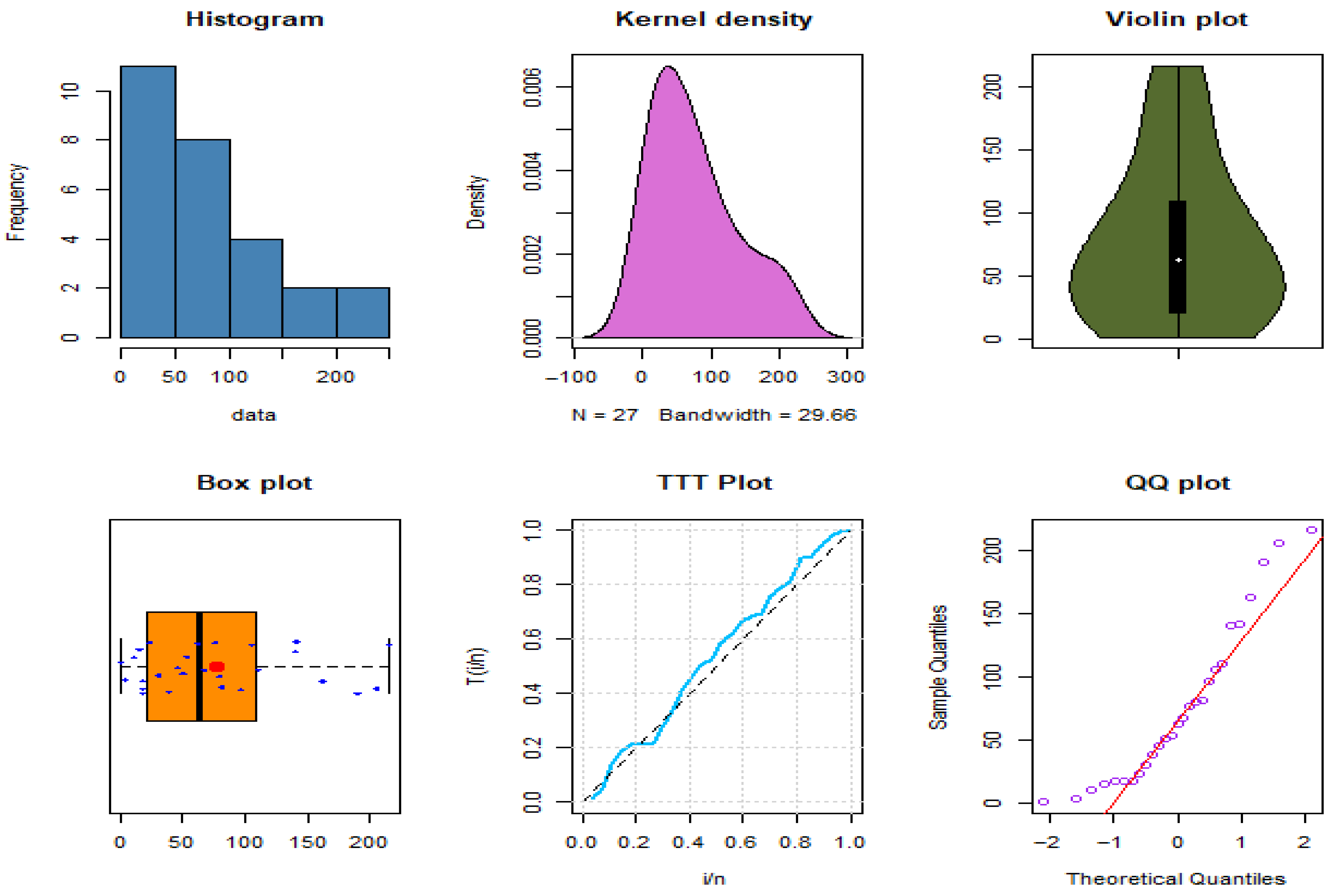
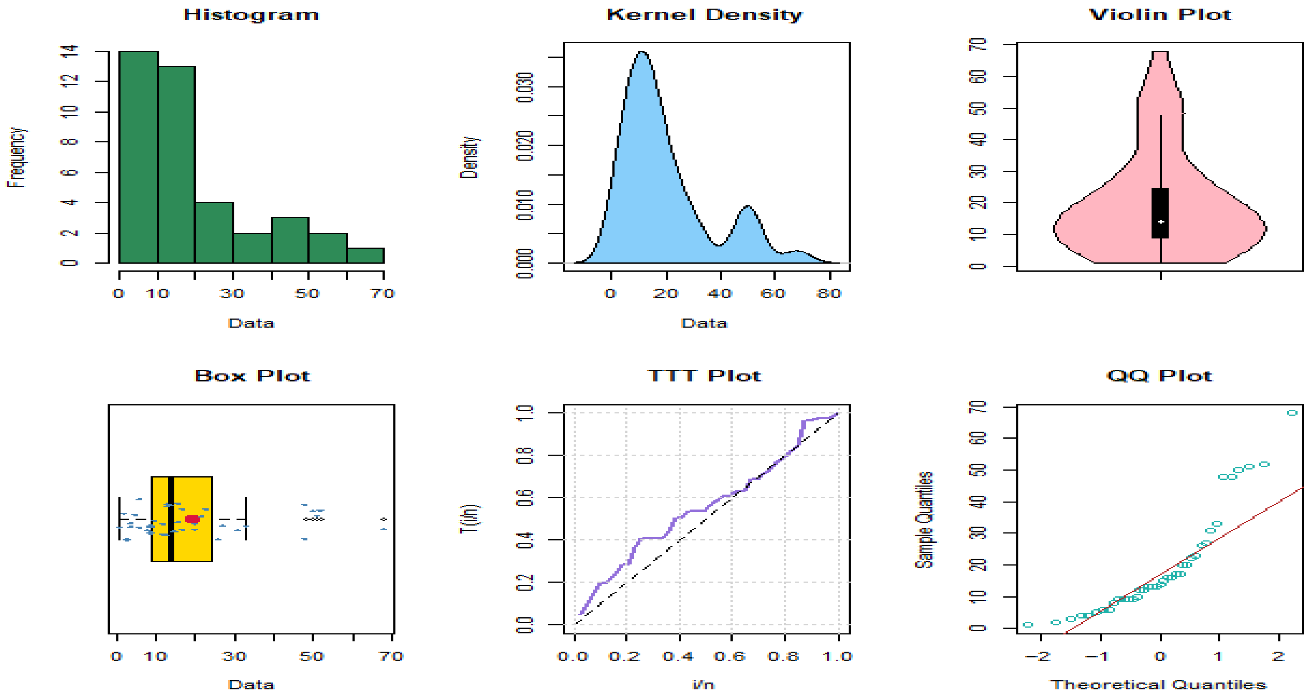
II	39	19.539	14	272.466	1.2877	3.7979	67	1	68

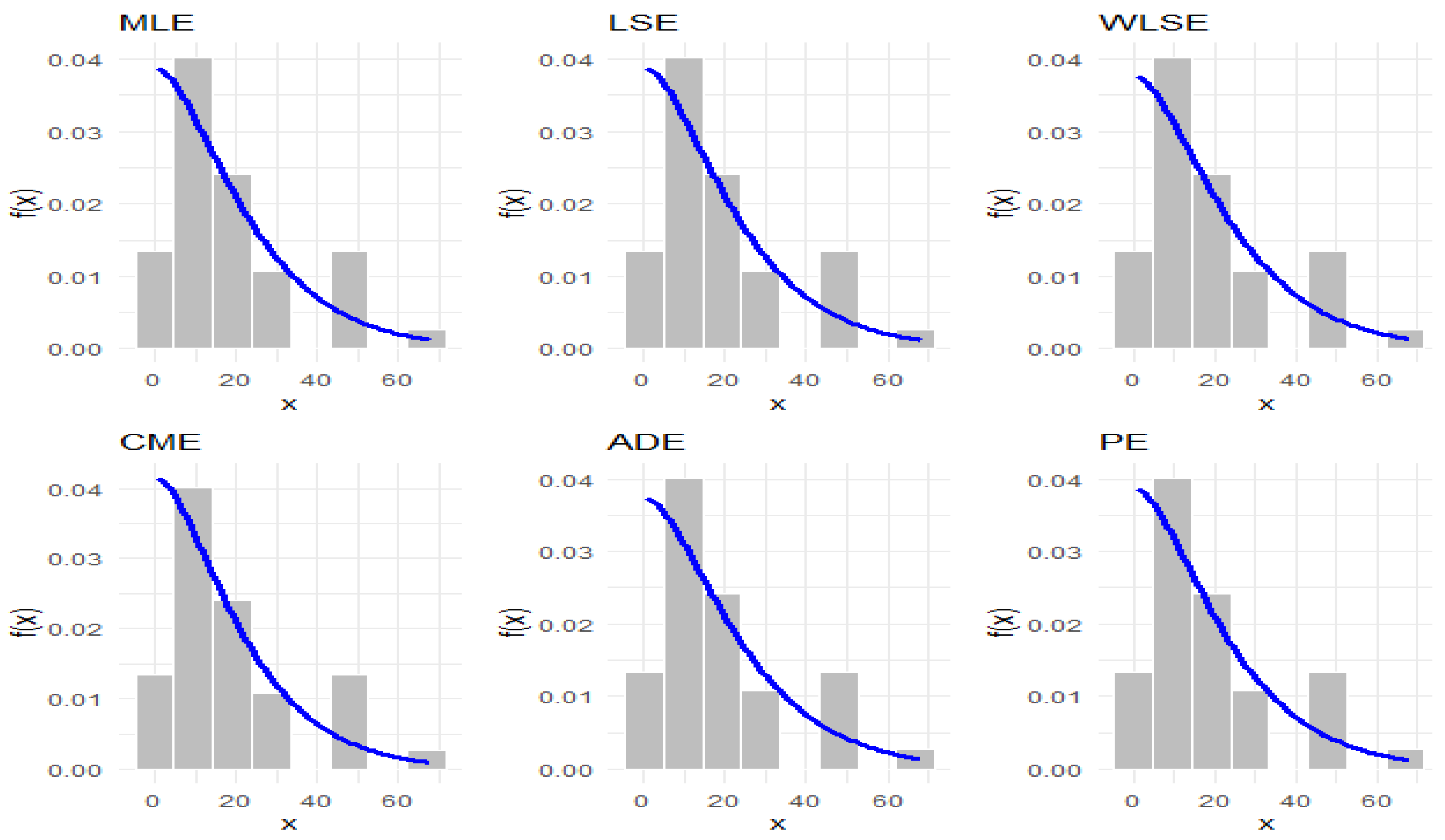
primarily examines the two datasets. Figure 4 and Figure 5 present graphical summaries of the datasets through quantile–quantile (QQ) plots, violin plots, box plots, histograms, kernel density estimates, and total time on test (TTT) plots. The results suggest that the first dataset follows a right-skewed, non-normal distribution with the presence of outliers and a bathtub-shaped hazard rate function (HRF). Similarly, the second dataset also displays right skewness, several outliers, and a bathtub-shaped HRF. The IALD, as established in the theoretical findings, can accommodate these properties.

This comparative analysis thoroughly assesses the IALD against several competing models, namely the Ailamujia (AL) [17], inverse power Ailamujia (IPAL) [25], Ishita (ISH) [41], generalized inverted exponential (GIEx) [42], and Sujatha (SU) [43] distributions. Parameter estimation and goodness-of-fit assessments were conducted using the maximum likelihood method within the R programming environment. The parameter estimates and their standard errors are reported in

Table 10. Results of MLE estimates with standard errors for dataset I.

Models	$\mathbf{Est}. \mathbf{of} \left(\mathit{\alpha }\right)$	$\mathbf{SE} \left(\widehat{\mathit{\alpha }}\right)$	$\mathbf{Est}. \mathbf{of} \left(\mathit{\lambda }\right)$	$\mathbf{SE} \left(\widehat{\mathit{\lambda }}\right)$
IAL	0.0098	0.0016	-	-
IPAL	10.114	2.2076	0.4805	0.0609
AL	0.0131	0.0018	-	-
ISH	0.0391	0.0043	-	-
SU	0.0388	0.0042	-	-
GIEx	0.5334	0.1285	8.8043	2.8362

and

Table 11. Results of MLE estimates with standard errors for dataset II.

Models	$\mathbf{Est}. \mathbf{of} \left(\mathit{\alpha }\right)$	$\mathbf{SE} \left(\widehat{\mathit{\alpha }}\right)$	$\mathbf{Est}. \mathbf{of} \left(\mathit{\lambda }\right)$	$\mathbf{SE} \left(\widehat{\mathit{\lambda }}\right)$
IAL	0.0388	0.0054	-	-
IPAL	9.8306	1.814	0.7025	0.0769
AL	0.0512	0.0058	-	-
ISH	0.1536	0.0142	-	-
SU	0.1489	0.0137	-	-
GIEx	1.2389	0.2865	9.4556	1.9875

.

Model selection was based on a range of statistical criteria, including the Akaike information criterion (S₁), Bayesian information criterion (S₂), corrected Akaike information criterion (S₃), Hannan–Quinn information criterion (S4), Kolmogorov–Smirnov distance (S₅) with associated p-value (S₆), and the Cramér–von Mises statistic (S₇). As shown in

Table 12. Results of goodness of fit of the IALD for dataset I.

Models	S1	S2	S3	S4	S5	S6	S7
IAL	289.688	290.984	289.848	290.074	0.087	0.988	0.023
IPAL	308.217	310.808	308.717	308.987	0.178	0.357	0.216
AL	296.712	298.008	296.872	297.097	0.179	0.356	0.132
ISH	312.081	313.377	312.241	312.466	0.227	0.123	0.302
SU	309.254	310.550	309.414	309.639	0.225	0.131	0.294
GIEx	320.629	323.221	321.129	321.399	0.257	0.092	0.591

and

Table 13. Outcomes of goodness of fit of the IALD for dataset II.

Models	S1	S2	S3	S4	S5	S6	S7
IAL	310.072	311.736	310.180	310.669	0.098	0.849	0.071
IPAL	319.722	323.049	320.055	320.916	0.149	0.354	0.141
AL	311.259	313.002	311.423	311.935	0.122	0.607	0.124
ISH	321.718	323.381	321.826	322.315	0.171	0.209	0.358
SU	318.405	320.068	318.513	319.002	0.159	0.279	0.319
GIEx	323.49	326.817	323.823	324.684	0.183	0.149	0.244

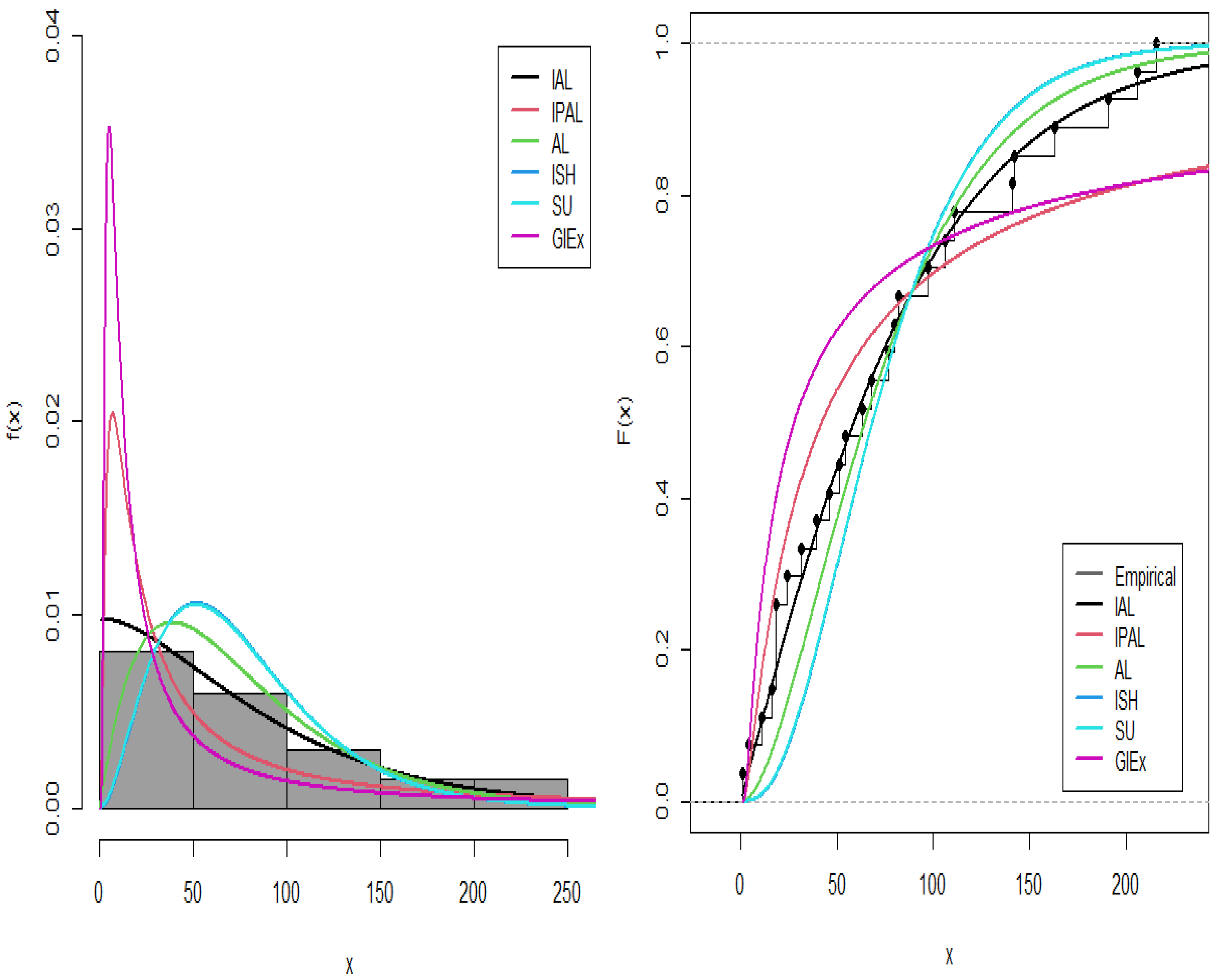
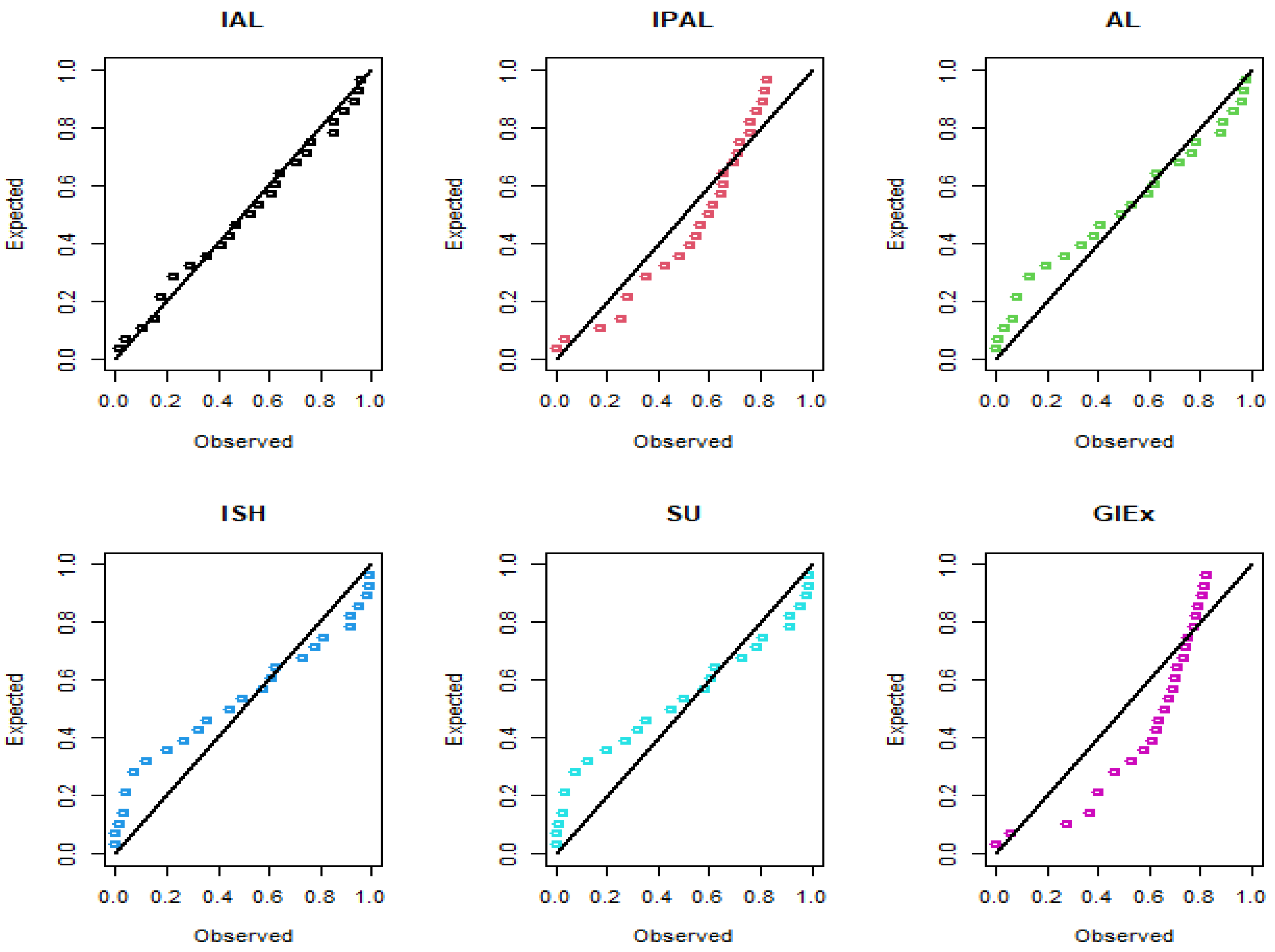
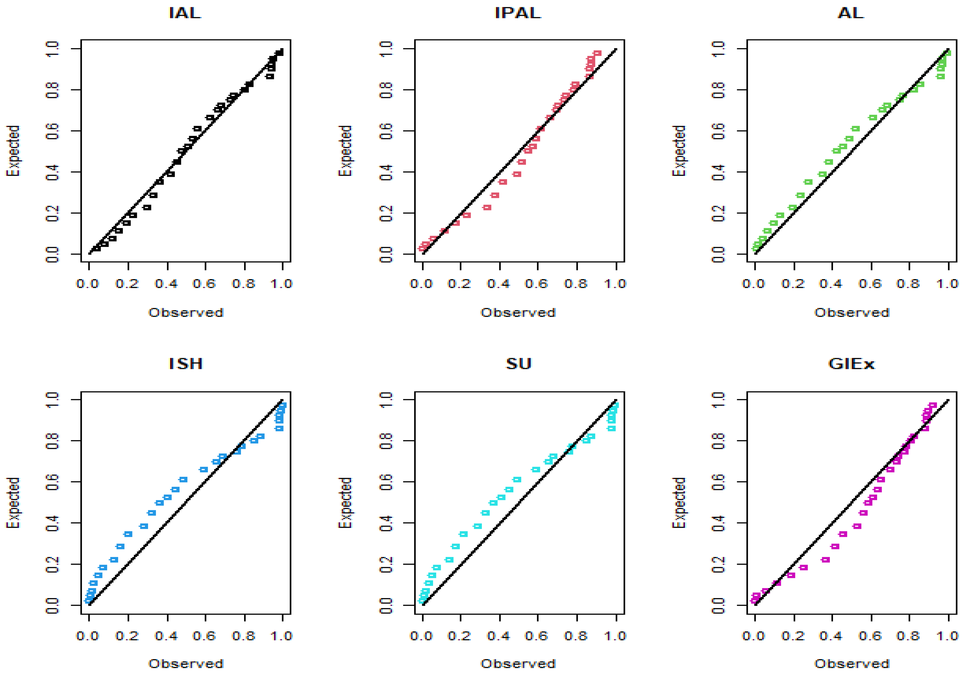
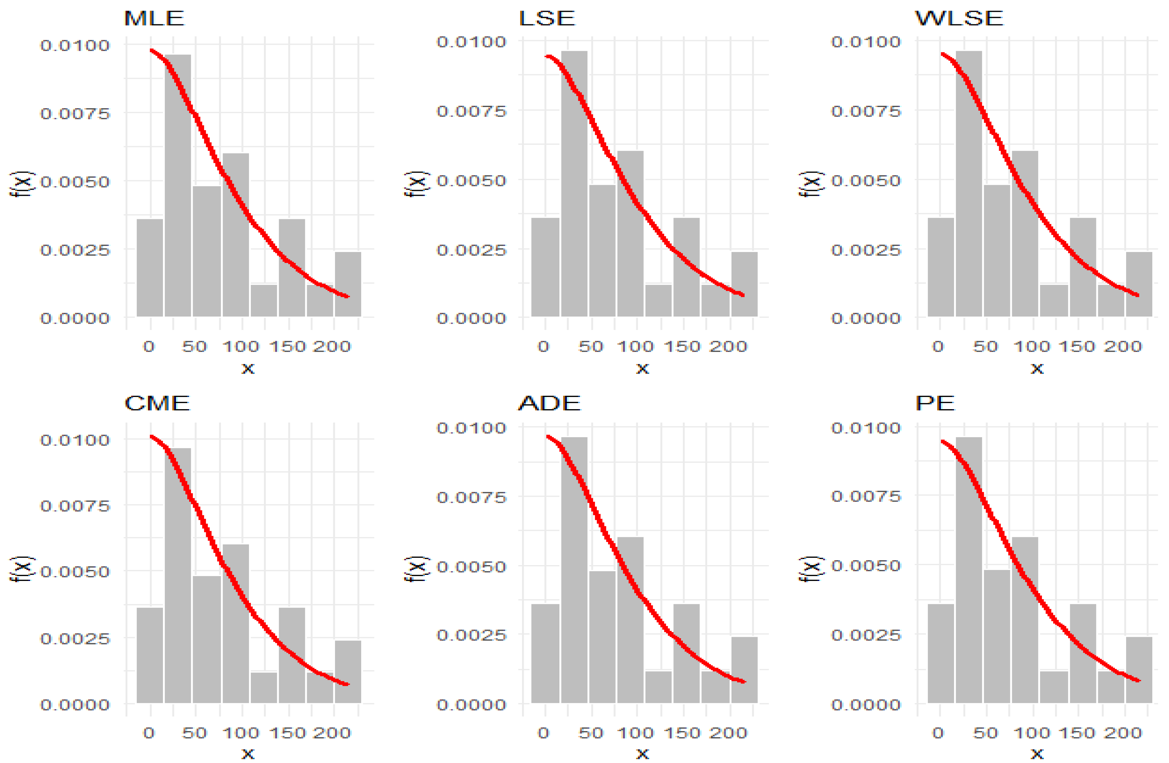
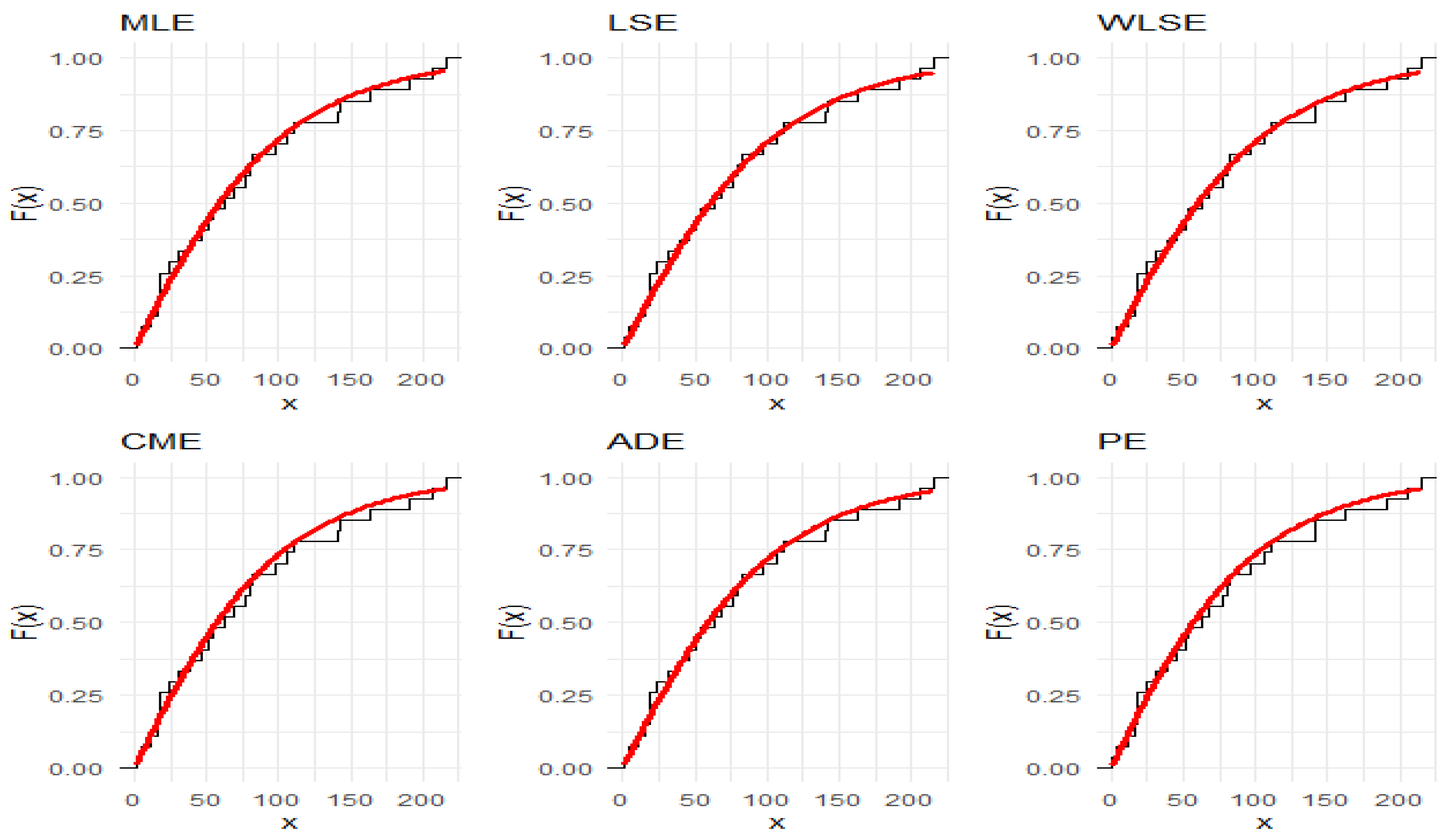
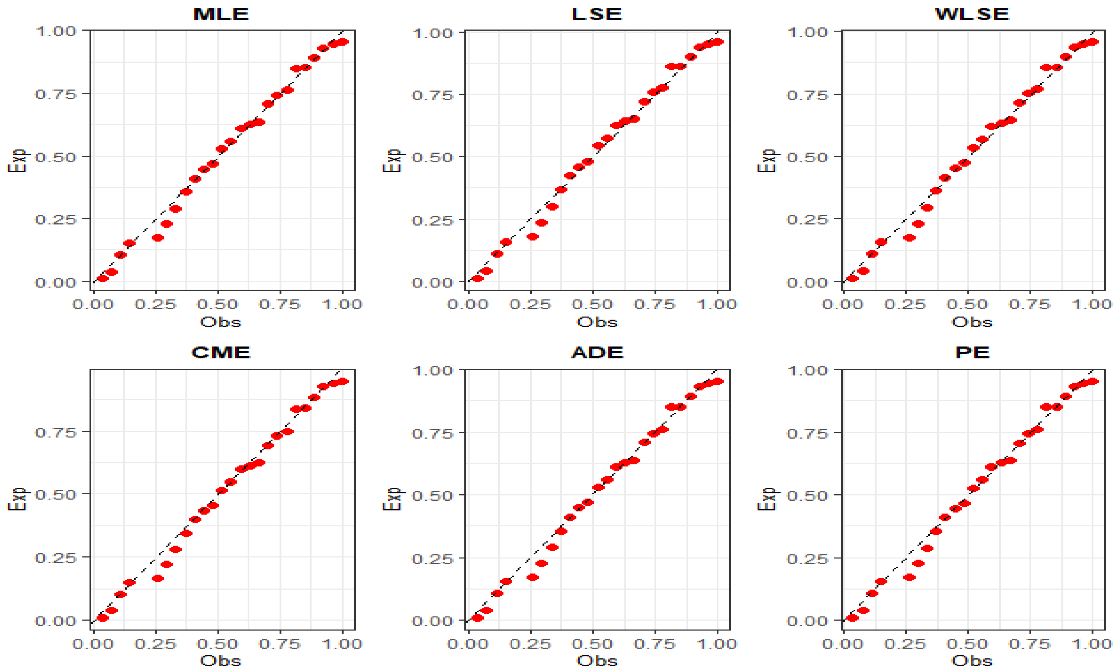
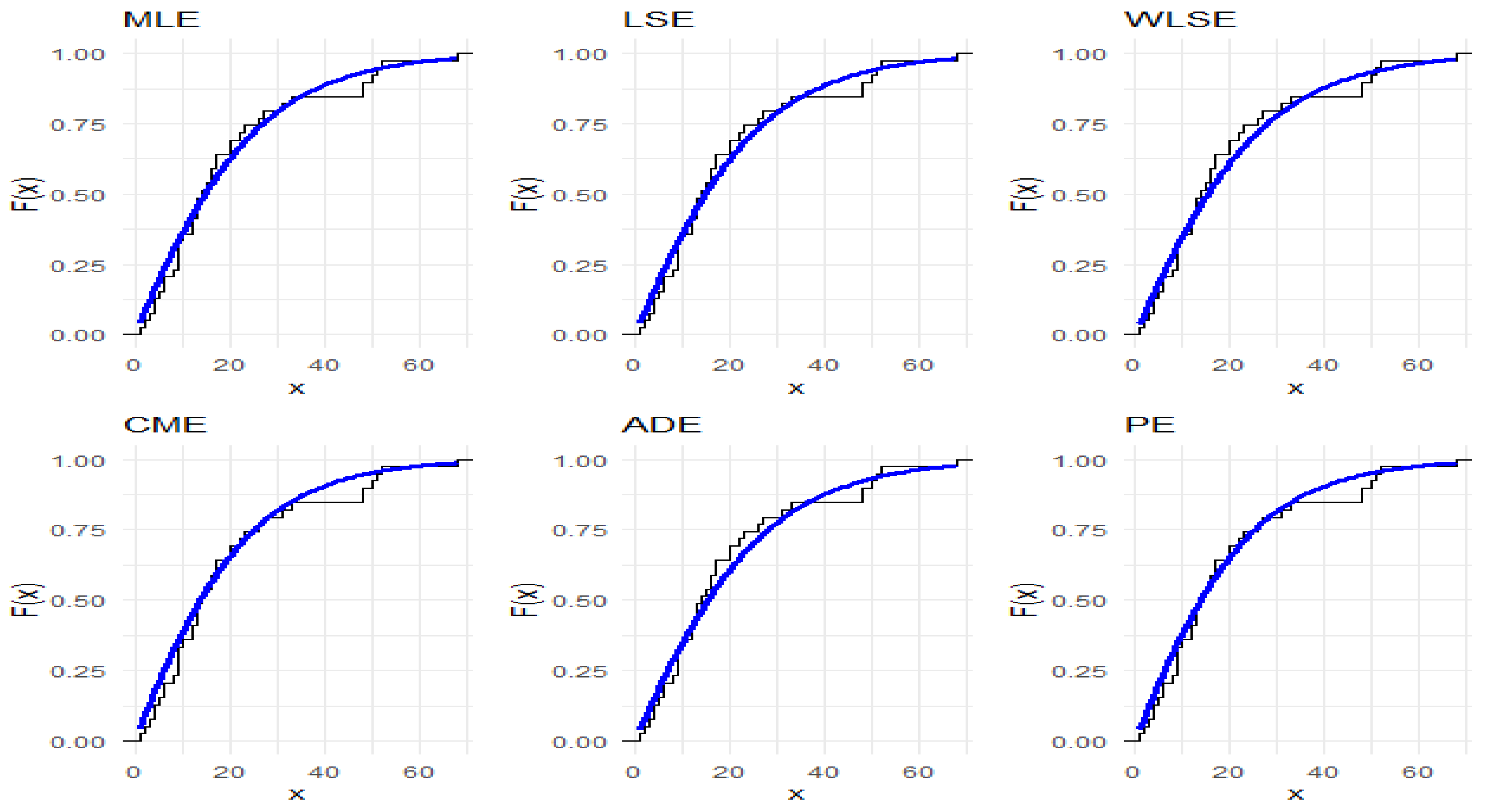
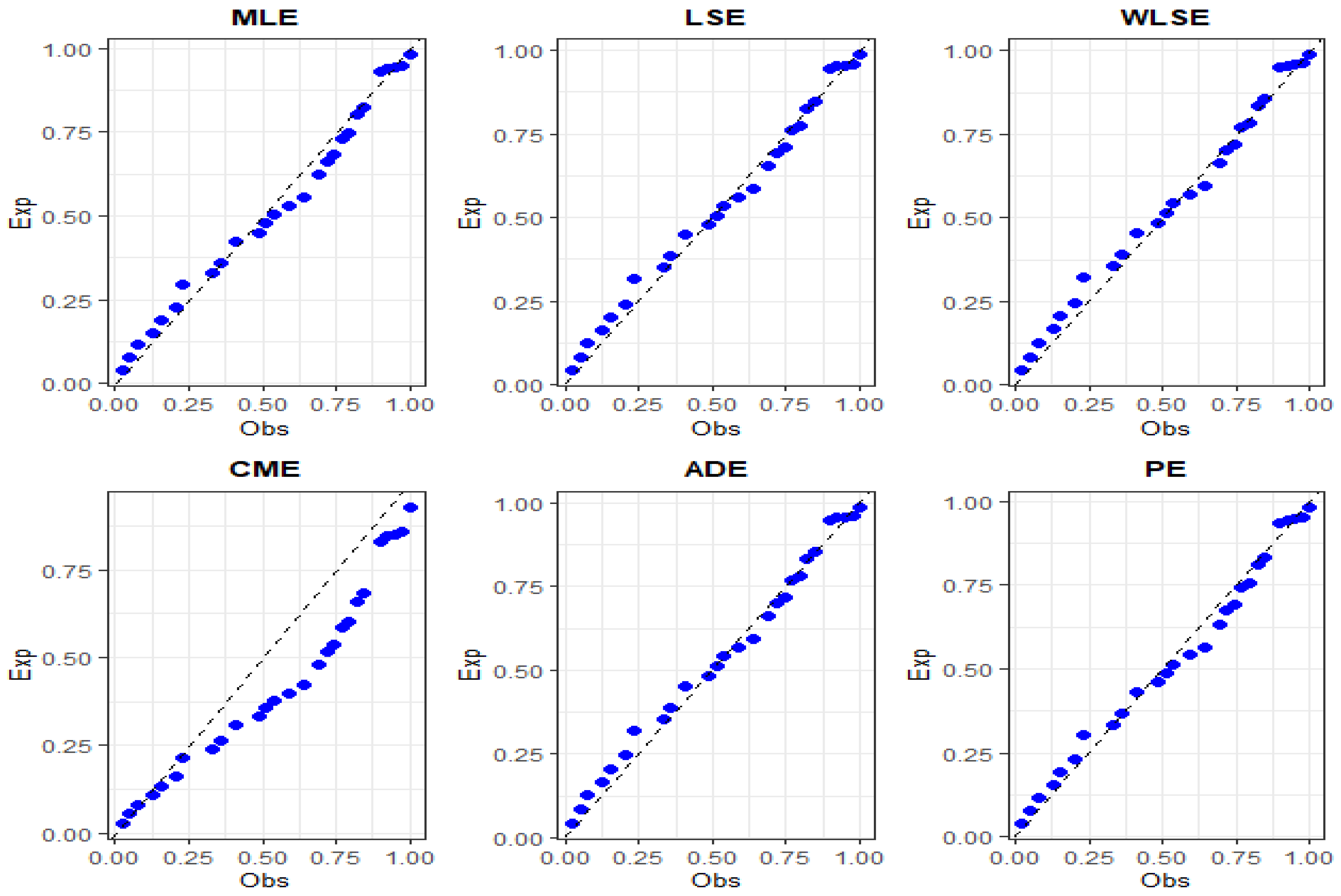
, the IALD outperforms all competitors, achieving the smallest values for S₁, S₂, S₃, S₄, S₅, S₆, and S₇, along with the largest value of S6. Additionally, graphical comparisons are presented in Figure 6 and Figure 7, which display fitted densities, empirical cumulative distribution functions, and P–P plots, while Figure 8, Figure 9, Figure 10, Figure 11, Figure 12 and Figure 13 offer visual comparisons of the two datasets with their corresponding fitted PDFs, CDFs, and P–P plots.

The comparative goodness-of-fit results confirm that the IALD consistently outperforms established lifetime models, including the Ailamujia, inverse power Ailamujia, Ishita, generalized inverted exponential, and Sujatha distributions. This superior performance is evidenced by lower values of AIC, BIC, HQIC, and Cramér–von Mises statistics, and higher K–S p-values, across both biomedical and industrial datasets.

7. Conclusions

In this study, we introduced the Induced Ailamujia Lifetime Distribution (IALD) as a flexible generalization of the Ailamujia distribution to overcome limitations in modeling complex lifetime and reliability data. The IALD can take a wide range of shapes, making it suitable for heterogeneous datasets where traditional models may fail. Several statistical properties were derived, including reliability measures, moments, quantile and generating functions, probability weighted moments, and entropy measures.

Different parameter estimation methods were applied and evaluated through simulation and real data analysis. The results confirmed the superior goodness-of-fit of the IALD compared to well-known lifetime models, underscoring its novelty and practical value in biomedical, engineering, and reliability studies. Finally, an important practical step is the development of software packages (e.g., in R14 or Python14) to provide user-friendly tools for density evaluation, parameter estimation, simulation, and goodness-of-fit testing, thereby enhancing the accessibility and applicability of the IALD in real-world research.

For future work, the IALD can be extended in multiple directions. Potential avenues include developing regression-type models, Bayesian inference approaches, and multivariate or hierarchical forms. Expanding comparisons to a broader range of distributions and applying the model to larger and more diverse datasets will further validate its robustness. Beyond reliability and biomedical studies, the IALD also shows promise in fields such as finance and social sciences, where data often displays skewness and heavy tails.