Bi-Objective Portfolio Optimization Under ESG Volatility via a MOPSO-Deep Learning Algorithm

Abstract

In this paper, we tackle a bi-objective optimization problem in which we aim to maximize the portfolio diversification and, at the same time, minimize the portfolio volatility, where the ESG (Environmental, Social, and Governance) information is incorporated. More specifically, we extend the standard portfolio volatility framework based on the financial aspects to a new paradigm where the sustainable credits are taken into account. In the portfolio’s construction, we consider the classical constraints concerning budget and box requirements. To deal with these new asset allocation models, in this paper, we develop an improved Multi-Objective Particle Swarm Optimizer (MOPSO) embedded with ad hoc repair and projection operators to satisfy the constraints. Moreover, we implement a deep learning architecture to improve the quality of estimating the portfolio diversification objective. Finally, we conduct empirical tests on datasets from three different countries’ markets to illustrate the effectiveness of the proposed strategies, accounting for various levels of ESG volatility.

1. Introduction

Diversification constitutes a key feature of portfolio management and has long been central to the decision-making process under risk and uncertainty in economics and finance [1]. In the framework of portfolio theory (e.g., the classical mean–variance model [2] and expected utility theory), diversification is based on asset dependence. Ceteris paribus, the weaker the positive dependence among portfolio assets, the greater is the portfolio diversification, thereby reducing simultaneous adverse performances across assets [3].

Therefore, the notion of diversification is linked to the portfolio risk. Nevertheless, the formalization of diversification remains conceptually complex, and debate persists regarding the most appropriate measure [4]. Recent contributions highlight the importance of constructing well-diversified portfolios and have proposed different approaches, such as Risk Parity, and entropy-based measures (see, e.g., [5,6]). Recently, the academic literature has underlined the diversification benefits of sustainable investments, particularly when green assets are incorporated into traditional bond and equity portfolios. Hoepner [7], for instance, states that Environmental, Social, and Governance (ESG) criteria can strengthen portfolio diversification by mitigating specific asset risks.

ESG scores offer a comprehensive evaluation of a company’s performance across the Environmental (E), Social (S), and Governance (G) dimensions, providing a measure of exposure to non-financial risks and long-term opportunities related to sustainable practices. The environmental pillar reflects the impact on natural resources and emissions; the social pillar captures aspects such as labor standards and stakeholder relationships; while the governance pillar measures the quality of corporate management and shareholder rights.

According to a report from Morgan Stanley (https://www.morganstanley.com/content/dam/msdotcom/en/assets/pdfs/Sustainable-Reality_2022_Final_CRC-5440003.pdf, (accessed on 11 August 2025)), in August 2020, the market value of sustainable funds surpassed USD 1 trillion for the first time. Both institutional and retail investors increasingly allocate capital to ESG-linked securities, driven by social pressures, ethical motivations, and climate-related awareness. While early approaches relied just on screening criteria, recent strategies have shifted toward ESG integration, reflecting heightened sensitivity to environmental and governance issues [8] (see also references therein). In this setting, ESG-linked signals start to acquire an interest comparable to the traditional financial indicators. For example, ESG signals related to the volatility of ESG scores may track a new source of systematic risk.

Such considerations enter into a classical multi-objective paradigm, where competing criteria must be jointly optimized.

Since the seminal contribution of Harry Markowitz in the 1950s [2], introducing the mean–variance portfolio selection framework, multi-optimization models have become fundamental tools in financial decision-making. Indeed, the domains of finance and insurance present substantial challenges for the design and implementation of advanced optimization methodologies. These challenges arise from the uncertainty and dynamic nature of financial systems, the multiplicity of stakeholders involved, the complexity characterizing global financial markets, the wide variety of financial products, and the increasing availability of large-scale data for analysis. Within this context, multi-objective optimization models are particularly relevant, where a unique optimal solution does not exist, and decision-makers’ preferences play a crucial role in selecting among Pareto-efficient alternatives. An example is the classical portfolio selection problem, where risk and return typically serve as the two primary criteria. This bi-objective framework has been extensively studied in the literature and is widely employed in practice. Nevertheless, risk is a multi-faceted notion with different origins, including systematic, unsystematic, and systemic sources, which have motivated the development of diverse risk measures extending beyond return variance. In addition, organizational and investor-specific policies (e.g., liquidity requirements, diversification preferences) and emerging considerations such as corporate social responsibility and regulatory compliance increasingly influence financial decision-making. The coexistence of these heterogeneous and often conflicting dimensions gives rise to practical challenges, and therefore the importance of the multi-objective optimization (see, e.g., [9,10,11], and references therein).

One of the first contributions to sustainable portfolio optimization problems incorporates ESG considerations as constraints within the classical Markowitz mean–variance model (see [12]). A significant advancement has been achieved by Utz et al. [13], who introduced sustainability as an objective function of the optimization problem, extending the efficient frontier into the tri-dimensional variance-profit-sustainability space. In this direction, the research activity has increased noticeably, with some approaches aiming to minimize risk and maximize diversification, and others integrating ESG criteria into classical financial metrics such as the mean, Sharpe ratio, and tracking error (see, e.g., [14,15,16,17,18]).

The present study contributes to this growing literature by introducing a novel bi-objective portfolio optimization framework that aims to minimize an augmented volatility, where ESG signals related to the volatility of ESG scores are incorporated, and to maximize the portfolio diversification à la Carmichael–Koumou–Moran [19].

To address this optimization problem, we develop a hybrid Multi-Objective Particle Swarm Optimization (MOPSO) algorithm, enhanced with a deep learning architecture and a tailored constraint-handling mechanism. For further details, we refer to Section 2 and Section 4.

Therefore, the novelties of this manuscript are threefold:

(i)

We introduce as the objective function an augmented portfolio volatility, where the standard financial volatility is expanded with ESG volatility signals via a sustainable-risk-aversion parameter;

(ii)

We analyze the interplay between this new augmented volatility and the portfolio diversification à la Carmichael–Koumou–Moran;

(iii)

We develop an improved MOPSO solver with a suitable project-and-repair mechanism to satisfy the constraints, which is also enhanced by a Long Short-Term Memory (LSTM) neural network architecture to better estimate the diversification measure.

It should be noted that, among the common approaches in the literature related to the use of ESG scores (screening, constraints, or objective-function integration), our contribution is in line with the third category, as ESG information is directly incorporated into the objective function through the augmented volatility measure (see, e.g., [8,20], and references therein.)

Findings from empirical analysis indicate that the introduction of the ESG component tends to generate more diversified portfolios, compared with the case in which purely financial risk is considered.

This work could also give some hints for the sustainable credits literature. Indeed, the ESG factors not only contribute to long-term value creation but also generate positive externalities for the broader socioeconomic environment. However, the efficient incorporation of such information into market valuations remains uncertain. Zeidan and Onabolu [21] state that sustainability credit scoring systems, which operate analogously to conventional credit rating models, represent an effective mechanism to enhance their lending practices. Such a framework should be designed to capture the full spectrum of potential outcomes by integrating both positive and negative potential interactions between environmental and social determinants and financial performance, rather than focusing exclusively on downside risks (see, e.g., [22,23,24]).

The remainder of the paper is then structured as follows. In the next section, we review the literature concerning the MOPSO solver and the deep-learning architecture. Section 3 introduces the mathematical model and its justification, while Section 4 presents the characteristics of the MOPSO algorithm and the LSTM design. Section 5 provides results related to the monthly efficient frontiers, describing the best trade-off between the augmented volatility and the portfolio diversification, and the profitability analysis of different strategies depending on a sustainable-risk-aversion parameter tested on three datasets. Section 6 offers concluding remarks and suggestions for future research directions. Finally, in Appendix A one could find the normality checks for the data and the goodness-of-fit tests for the LSTM architecture, while Appendix B is devoted to a deeper analysis concerning the Pareto front outcomes and the optimal weight allocations.

2. Literature Review

This section is devoted to a brief overview of the literature concerning the MOPSO solver and the neural network (NN) architecture.

2.1. MOPSO Solver

This section is focused on the literature linked to the Particle Swarm Optimization (PSO) algorithm and its extension to the multi-objective framework. The PSO has been initially designed for single-objective optimization in [25], and it has gained popularity due to its simplicity in implementation, efficiency, and ability to handle complicated search spaces. Over time, PSO has been improved to overcome the stagnation and local trapping issues. As a result, mutation and repair mechanics have been introduced (see, e.g., [26,27,28,29,30]). For a more recent application of a hybrid version of PSO with neural network architecture, we refer to [20], where the neural component is employed to calibrate the three key PSO parameters ($c_1$, $c_2$, w) and to generate estimates that directly feed into the objective function of the optimization problem.

Since real-world problems typically involve multiple decision objectives, the PSO paradigm has been extended to the Multi-Objective Particle Swarm Optimization (MOPSO). In this context, new strategies appear as the Pareto dominance, the leader selection mechanism, and the external archive based on the crowding distance, in order to effectively navigate in the multi-dimensional decision space.

The pioneering paper concerning the extension of PSO to multi-objective optimization problems goes back to [31]. In such a study, it has been shown that swarm-based approaches can handle multiple conflicting objectives effectively, laying the foundation for later adaptations. Afterward, in [32], the authors introduced a MOPSO algorithm incorporating Pareto dominance and an external archive to maintain solution diversity and improve convergence. The use of a double mutation strategy has been implemented in a subsequent paper [33]. In [34], a comparative analysis of MOPSO algorithms, highlighting challenges in maintaining solution diversity, is presented. The study introduces a MOPSO variant, which incorporates a velocity constraint mechanism to improve stability and diversity preservation. These findings highlight the importance of the clamping and repair mechanism in the MOPSO framework. Finally, in reference [35] is presented a detailed review of MOPSO advancements, categorizing modifications based on leader selection, archive repository, and velocity updates. They have stressed the fundamental role of mutation operators, adaptive mechanisms, and hybrid approaches in improving the standard MOPSO solver.

2.2. Neural Network Architecture

Neural networks (NN) represent a class of deep-learning-based models inspired by the functioning mechanism of the human brain. They are composed of interconnected computational units, called neurons, organized into multiple layers. Each neuron processes incoming data and transmits the transformed information to the following layers in order to provide an outcome that is as accurate as possible.

During the last decades, neural networks have become increasingly relevant in finance thanks to their ability to model non-linear relationships and to effectively handle large-scale datasets (see [36,37], among others). Furthermore, they are known as useful and potential tools for estimating quantities when no closed-form formula exists or can be applied, making them powerful approximation models. In addition to finance, neural networks have also been successfully applied in a wide range of fields, including computer vision [38] and natural language processing [39], making them a versatile tool for different goals.

In the literature, different types of architectures have been defined according to the structure of connections among units. Limiting our attention to the models at the basis of the architecture adopted in this work, the starting point is represented by Feed-Forward (FF) neural networks, in which information propagates only forward, from the input layer to the output layer [40]. In this type of network, each layer processes the information from the previous one, progressively extracting outcomes that are functional to the learning task. These networks represent the foundation for the evolution of neural architectures and a reference for numerous applications.

A natural extension is provided by Recurrent Neural Networks (RNNs), introduced by Elman [41]. Unlike the FF networks, they are characterized by cyclic connections that allow the output generated in previous steps to be reused as input. In this case, predictions take into account the past information, making these architectures particularly suited for processing temporal or sequential data. However, training a vanilla RNN is often limited by the vanishing gradient issue, which makes this architecture less effective in the presence of long-term dependencies.

To overcome these limitations, more sophisticated architectures have been developed, including the Long Short-Term Memory (LSTM) networks [42]. LSTM, compared with the RNNs, integrates additional memory cells that are able to store and process the long-term information [43]. In the literature, this type of network has shown promising results in complex domains, such as machine translation or modeling music and speech sequences, leading to their following application in other fields, including finance (another widely used variant is represented by Gated Recurrent Units (GRUs), introduced by Cho et al. [44], which simplify the structure of LSTM by reducing the number of parameters and, in some cases, show greater efficiency).

3. Mathematical Problem

This section is dedicated to the description of the theoretical framework for our optimization task, and we also present the motivation behind the problem.

The sustainable portfolio bi-objective optimization problem can be mathematically written at every fixed time $t=1,\dots ,T$ as follows,

$$\begin{array}{cc}\hfill & \underset{\mathbf{w}}{min}\sum _{i,j=1}^N{w}_i{w}_j\left(\lambda {\sigma }_{ij}^{fin}+(1-\lambda ){\sigma }_{ij}^{ESG}\right)(\mathrm{minimize}\mathrm{the}\mathrm{augmented}\mathrm{volatility})\hfill \\ \hfill & \underset{\mathbf{w}}{max}{\displaystyle \frac{1}{2}}\sum _{i,j=1}^N{d}_{ij}{w}_i{w}_j(\mathrm{maximize}\mathrm{the}\mathrm{portfolio}\mathrm{diversification})\hfill \end{array}$$

(1)

such that the following constraints are satisfied:

$$\begin{array}{cc}\hfill & \sum _{i=1}^N{w}_i=1\left(\mathrm{budget}\right)\hfill \end{array}$$

(2)

$$\begin{array}{cc}\hfill & 0\le w_i\le 1i=1,\dots ,n\left(\mathrm{box}\right).\hfill \end{array}$$

(3)

The vector $\mathbf{w}=(w_1,\dots ,w_N)\in {\mathbb{R}}^N$ represents the N weights of a portfolio, where N indicates the number of assets of the investable universe and $w_i\in \mathbb{R}$ is the proportion of wealth invested in the i-th asset, for all $i=1,\dots ,N$. Each i-th asset is associated to a real-valued return (per period) $r_i$, and each pair of assets $(i,j)$ are associated to a real-valued financial covariance ${\sigma }_{ij}^{fin}$. The matrix ${\Sigma }^{fin}\in {\mathbb{R}}^{N\times N}$ is symmetric and the diagonal element ${\sigma }_{ii}$ is the financial variance of i-th assets. The matrix ${\Sigma }^{ESG}$ is the sustainable counterpart, where ${\Sigma }^{ESG}={\left({\sigma }_{ij}^{ESG}\right)}_{i,j=1}^N$. To build such a matrix ${\Sigma }^{ESG}$, we adopt an approach analogous to [45], in which a return-like quantity is derived using ESG data as a proxy for a company’s sustainability. Following [46], we treat sustainability-related returns as stochastic, since managers’ good practices are ex-ante impossible to predict. For the empirical implementation, we employ ESG ratings from Refinitiv, which are reported on a 0–100 scale. While this standardized scaling facilitates the evaluation of a firm’s relative sustainability performance, we assess whether a firm’s ESG rating outperforms or underperforms with respect to industry standards over successive periods. Accordingly, we define the sustainable-return counterpart as the rate of return in ESG performance for each asset i at time t. Specifically, following [45], let the standardized relative sustainability performance be

$$s{p}_i^{\left(t\right)}={\displaystyle \frac{ES{G}_i^{\left(t\right)}}{{\overline{ESG}}^{\left(t\right)}}},$$

where ${\overline{ESG}}^{\left(t\right)}$ is the average ESG rating of all companies in the current rating universe across industries. Therefore, we can define the sustainable-return as

$$s{r}_i^{\left(t\right)}={\displaystyle \frac{s{p}_i^{\left(t\right)}}{s{p}_i^{(t-1)}}}-1.$$

A positive sustainable-return indicates that the firm has improved its relative ESG rating over a given period, thereby reflecting progress in the adoption of ESG-oriented practices. Hence, analogously to the financial counterpart, we build the sustainable-covariance matrix, denoted by ${\Sigma }^{ESG}$, which captures the dynamics of ESG-related risk over time. Formally, for each asset i the expected return of ESG at time t is computed over the past L observations as

$${\overline{sr}}_i^{\left(t\right)}={\displaystyle \frac{1}{L}}\sum _{\ell =1}^{L}s{r}_i^{(t-\ell )}.$$

The ESG covariance (it should be noted that if $i=j$, ${\sigma }_{ii}^{ESG,\left(t\right)}$ corresponds to the ESG variance of asset i) between assets i and j at the same time is defined by

$${\sigma }_{ij}^{ESG,\left(t\right)}={\displaystyle \frac{1}{L}}\sum _{\ell =1}^L\left(s{r}_i^{(t-\ell )}-{\overline{sr}}_i^{\left(t\right)}\right)\left(s{r}_j^{(t-\ell )}-{\overline{sr}}_j^{\left(t\right)}\right).$$

Accordingly, the ESG covariance matrix at time t is

$${\Sigma }^{ESG,\left(t\right)}={\left({\sigma }_{ij}^{ESG,\left(t\right)}\right)}_{i,j=1}^N$$

and the ESG volatility of asset i is given by the standard deviation

$${\sigma }_i^{ESG,\left(t\right)}=\sqrt{{\sigma }_{ii}^{ESG,\left(t\right)}}.$$

For the sake of simplicity, in the following we drop the explicit time index and simply write ${\Sigma }^{ESG}={\left({\sigma }_{ij}^{ESG}\right)}_{i,j=1}^N$.

By construction, ESG volatility satisfies the standard properties of a variability index (see, e.g., [47] among others): (i) non-negativity and (ii) being equal to zero if and only if all ESG returns are identical across the sample. Furthermore, it also satisfies homogeneity under linear transformations, namely $\sigma \left(Y\right)=\left|\alpha \right|\sigma \left(X\right)$ if $Y=\alpha X+\beta$.

Given this framework, the augmented volatility to be minimized in (1) is then given by the combination of the two matrices ${\Sigma }^{fin}$ and ${\Sigma }^{ESG}$, where $\lambda \in [0,1]$ is the sustainable-risk-aversion parameter which describes the agent’s appetite for the ESG volatility information. It is worth stressing that, since ESG returns are defined in analogy with financial returns, both ${\Sigma }^{fin}$ and ${\Sigma }^{ESG}$ are expressed in homogeneous units of variability. Hence, $\lambda$ acts as a preference parameter between financial and sustainable risk.

As a second aim, we aim to maximize the diversification of the portfolio, which is encoded through the dissimilarity matrix $D={\left(d_{ij}\right)}_{i,j=1}^N$, where $d_{ij}$ measures the degree of dissimilarity between asset i and asset j. Following the approach proposed in [19], this dissimilarity is defined as

$$d_{ij}=(1-{\rho }_{ij}){\left({\displaystyle \frac{{\sum }_{k=1}^N{\mathrm{CVaR}}_{\alpha }\left(r_k\right)}{N·{\mathrm{CVaR}}_{\alpha }\left(r_i\right)}}\right)}^{{\displaystyle \frac{1}{2}}}·{\left({\displaystyle \frac{{\sum }_{k=1}^N{\mathrm{CVaR}}_{\alpha }\left(r_k\right)}{N·{\mathrm{CVaR}}_{\alpha }\left(r_j\right)}}\right)}^{{\displaystyle \frac{1}{2}}}$$

(4)

with $\alpha =0.05$ and ${\rho }_{ij}$ is the Pearson correlation coefficient between asset i and asset j (this formulation implies that pairs of assets with low (or negative) correlations are associated with higher dissimilarity values, reflecting a high potential for diversification, as also stated in [19]). In (4), the notion of Conditional Value-at-Risk (CVaR) is introduced as

$${\mathrm{CVaR}}_{\alpha }\left(r_i\right)=\mathbb{E}[r_i\mid r_i\le {\mathrm{VaR}}_{\alpha }\left(r_i\right)]$$

where ${\mathrm{VaR}}_{\alpha }\left(r_i\right)=inf\{R\in \mathbb{R}:\mathbb{P}(r_i\le R)\ge \alpha \}$.

It is worth noting that the CVaR is a coherent risk measure (see, e.g., [48]) capturing the average tail loss, and $r_i$ has a continuous and strictly increasing distribution (see also [49]).

Finally, in (1) we consider the standard constraints given by the budget and box requirements. The budget constraint (2) translates the requirement that all the available capital has to be invested. At the same time, the weight of asset i has to be in the range $[0,1]$ in order to exclude short sales.

Remark 1.  

It is straightforward to show that the augmented matrix presented in the objective function of problem (1) is positive semidefinite since it is a convex combination of positive semidefinite matrices.

Remark 2.  

We underline that our optimization process is rebalanced month-by-month for a total of $T=60$ rebalancing phases. Rebalancing occurs on the last business day of each month, and trades are executed at the closing prices.

3.1. Motivation of the Problem

One of the two objectives of the optimization problem defined in (1) is minimizing the augmented volatility, which incorporates the uncertainty component associated with the variability of ESG scores. To motivate this choice, we explore the correlation structure among the ESG of the different constituents of a financial index. To better understand this exploration, in Figure 1 we show, for three financial indices—the Dow Jones Industrial (USA), the Euro Stoxx 50 (Europe), and the FTSE 100 (UK), provided by Refinitiv (www.refinitiv.com)—two heatmaps: one relating to the correlation matrix of the daily returns of assets (left side), and the latter referring to the correlation matrix of the ESG scores (right side). Pearson correlation coefficients of the two matrices are calculated on daily data over the period 2006–2020, and they express the degree of linear co-movement for each pair of securities, both from a financial perspective and from a sustainability point of view.

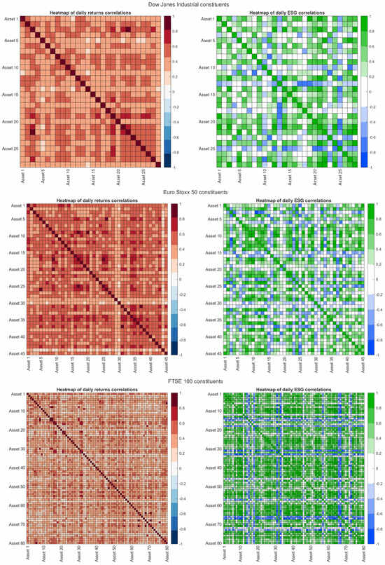
Figure 1. Heatmaps of correlation matrices of daily returns (left) and correlation matrices of ESG scores (right) for the constituents of the Dow Jones Industrials, Euro Stoxx 50, and FTSE 100 over 2006–2020.

For returns (maps on the left), as expected, correlations between couples of assets are mainly positive and medium-high, confirming that stocks belonging to the same market tend to move together in response to macroeconomic shocks and systemic factors.

On the other hand, the three maps relating to ESG variability are characterized by greater heterogeneity. It should be noted that there exist several blocks associated to positive correlations, which indicate similar trends for different pairs of stocks. Nevertheless, several correlations are almost absent or even negative, indicating that an improvement in the ESG profile of a company corresponds to a worsening in the same profile for another one. This phenomenon can be attributed to the different ways in which companies balance the environmental (E), corporate behavior (S), and governance (G) strategies to improve their ESG profile. As a result, ESG scores do not evolve independently over time, but follow a dynamic structure of interconnection among them. To take this dynamics into account, we introduce an augmented volatility, which combines the financial risk component with the sustainable one.

In the previous analysis, the heatmaps were created from the three different datasets, which cover the United States (Dow Jones Industrial), Europe (Euro Stoxx 50), and the United Kingdom (FTSE 100).

We focus on these three different markets that comprise the largest and most liquid stocks in their respective regions, making them suitable for portfolio construction and risk assessment. Furthermore, their different market structures and ESG disclosure practices enable us to test whether our bi-objective optimizer behaves consistently in each different geographical context.

Each dataset consists of daily prices and ESG ratings (provided by Refinitiv) covering the period from the 6th October 2006 to the 31st December 2020 for a total of 3715 observations. More details about the datasets can be found in Table 1.

Table 1. The three datasets with the corresponding number of observations, number of market constituents (N), and the corresponding currency.

Dataset Name	Daily Observations	Assets (N)	Currency
Dow Jones Industrial	3715	28	$
Euro Stoxx 50	3715	45	€
FTSE 100	3715	80	£

The empirical panel is balanced since only full-history assets are considered. Datasets are publicly available at [50].

More specifically, we employ an out-of-sample window, from January 2016 to December 2020, to point out the effects of the market changes on the behavior of the investments. Furthermore, the in-sample window is represented by the period from January 2012 to December 2015, updated in each rebalancing phase.

3.2. Scenario Generation Technique

To simulate the rate of returns, we use a bootstrap procedure [51]. More specifically, we consider a stationary bootstrap that employs a random block size (i.e., a set of consecutive scenarios) to bring some robustness with respect to the standard block bootstrap (which instead employs fixed block size). We start by selecting the optimal average block size $B^{*}$ through the technique presented in [52], which is fully automatic. Then, we randomly extract, from the in-sample data, a block of length $B^{*}$. We repeat this procedure until the extracted sample reaches the desired size H (we remark that H represents the number of business days in a month), adjusting the last block length if necessary.

Finally, we a simulated bootstrap sample of H rates of simple-return for each asset i, denoted as ${\widehat{r}}_i^{\left(t^{\prime }\right)}$, with $i=1,\dots ,N$ and $t^{\prime }=1,\dots ,H$. We calculate the simulated H-step ahead rate of simple-return of the i-th asset by ${\widehat{r}}_i^{\left(H\right)}={\prod }_{t^{\prime }=1}^H\left(1+{\widehat{r}}_i^{\left(t^{\prime }\right)}\right)$ and the simulated H-step ahead rate of simple-return of portfolio $\mathbf{w}$ in the following way, ${\widehat{r}}_{\mathbf{w}}^{\left(H\right)}={\sum }_{i=1}^N{w}_i{\widehat{r}}_i^{\left(H\right)}$. We repeat this procedure S times to have an estimate of the empirical distribution.

In this paper, the number of scenarios is set at 10,000. For all the details, we refer the interested reader to [52].

4. Overview of the Solver

We describe below the hybrid solver developed to tackle the bi-objective problem presented in (1). Firstly, we illustrate the structure of the MOPSO solver (implemented in MATLAB R2025a) with some improvements. Next, we design the LSTM architecture needed to effectively estimate the dissimilarity matrix.

4.1. MOPSO Description

Multi-Objective Particle Swarm Optimization (MOPSO) was introduced in an unpublished document and subsequently proposed by Moore and Chapman [31] as an extension of the standard PSO algorithm. MOPSO is specifically designed to tackle optimization problems involving multiple conflicting objectives, a common occurrence in real-world scenarios. Unlike single-objective optimization, where the goal is to find a single optimal solution, multi-objective optimization seeks to find a set of solutions that represent the trade-offs among competing objectives, the so-called Pareto front. We present in Figure 2 the flowchart of the algorithm.

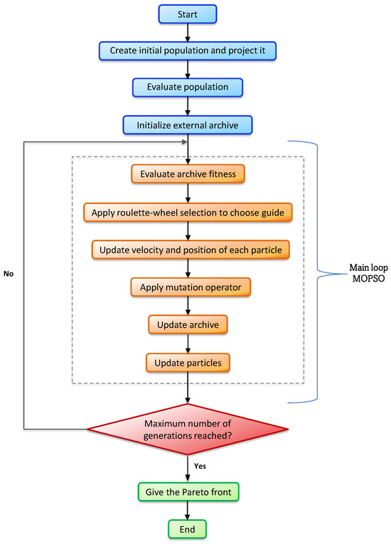
Figure 2. A graphical representation of the MOPSO solver.

While in the standard PSO algorithm, each particle has one global best position to track and move toward to, in MOPSO, each particle can have multiple potential leaders, each representing a different Pareto optimal solution. The particle selects one of these leaders at each iteration to update its position and velocity, allowing the swarm to explore multiple optimal regions of the solution space simultaneously. These multiple leaders are stored in an external archive. The archive serves as a repository for the best-found solutions, which are stored based on the Pareto dominance principle.

The archive plays a crucial role in ensuring that the solutions found by the swarm remain diverse and representative of the entire Pareto front. In this respect, we employ the Pareto dominance principle and the crowding distance mechanism (see [32]).

In addition to modifying the swarm dynamics, MOPSO also corrects the positions and velocities of the particles that exceed the boundaries. The velocity update rule is designed to balance exploration (searching for new regions of the solution space) with exploitation (refining already discovered solutions). By doing so, MOPSO is able to effectively navigate complex, multi-dimensional solution spaces and identify high-quality solutions that lie along the Pareto front.

Finally, to improve the basic MOPSO, we implement a mutation strategy that divides the swarm into three subgroups. The first subgroup is not affected by the mutation process, the second one is mutated through a uniform mutation, and the last one is enhanced via the mutation operator developed by Coello et al. in [32].

Algorithm 1 describes the pseudocode of the MOPSO algorithm.

Algorithm 1: Multi-Objective Particle Swarm Optimization (MOPSO)

1: Input: Number of particles $N_{pop}$, search space bounds $[0,1]$, maximum iterations $max\_iter$, inertia weight $\omega$, social coefficient $c_1$, and cognitive coefficient $c_2$ 2: Output: Pareto front archive with non-dominated solutions 3: Initialize $N_{pop}$ particles with random positions ${\mathbf{w}}^p$ and zero velocities ${\mathbf{v}}^p$ 4: Project the particles in the feasible region via (5) and (6) 5: Evaluate objective functions $f_1\left({\mathbf{w}}^p\right),f_2\left({\mathbf{w}}^p\right)$ in (1) for each particle p 6: Set personal best position ${\mathbf{w}}_{best}^p={\mathbf{w}}^p$ and cost $cos{t}_{best}^p=[f_1\left({\mathbf{w}}^p\right),f_2\left({\mathbf{w}}^p\right)]$ 7: Initialize archive to store non-dominated solutions 8: for $iter=1$ to $max\_iter$ do 9:    for each particle p do 10:      Select global best $gbest$ randomly from archive if not empty, otherwise from particles 11:      Update velocity component-wise: $v_i^p=\omega ·v_i^p+c_1·r_1·(gbes{t}_i-w_i^p)+c_2·r_2·(w_{best,i}^p-w_i^p)$ 12:      Update position component-wise: $w_i^p=w_i^p+v_i^p$ 13:      Apply the mutation mechanism with percentage $mu{t}_{\%}$ 14:      Correct the positions and velocities of the particles that exceed the boundaries and project them into the feasible region 15:      Evaluate objectives: $f_1\left({\mathbf{w}}^p\right),f_2\left({\mathbf{w}}^p\right)$ 16:      if current solution dominates personal best then 17:         Update personal best: ${\mathbf{w}}_{best}^p={\mathbf{w}}^p$ and $cos{t}_{best}^p=[f_1\left({\mathbf{w}}^p\right),f_2\left({\mathbf{w}}^p\right)]$ 18:      end if 19:      Update archive through the Pareto principle: 20:      Remove dominated solutions by ${\mathbf{w}}^p$ 21:      if ${\mathbf{w}}^p$ is not dominated by any archive member then 22:         Add ${\mathbf{w}}^p$ to archive 23:      end if 24:    end for 25:    if archive size exceeds $A_{max}$ then 26:      Reduce archive by crowding distance mechanism to maintain $A_{max}$ solutions 27:    end if 28: end for 29: Return: Archive containing Pareto optimal solutions

The initialization phase ensures that the swarm begins with a well-distributed set of candidate solutions with zero velocities. In line 3, each of the $N_{pop}$ particles, for $i=1,\dots ,N$, is initialized with a random position $w_i^p$ within the problem’s search bounds $[0,1]$ (in our context) and assigned a velocity $v_i^p=0$. In line 4, after defining the initial positions, the particles are projected into the feasible region through a project-and-repair mechanism (see [20]). For further details of such a process, we refer to Section “Project-and-Repair Mechanism”.

In line 5, the objective functions $f_1\left({\mathbf{w}}^p\right)$ and $f_2\left({\mathbf{w}}^p\right)$ of (1) are evaluated for each particle via the use of the LSTM framework (see Section 4.2). These function values determine the quality of the initial solutions.

In line 6, the personal best position ${\mathbf{w}}_{best}^p$ for each particle is set to its initial position, and its corresponding objective values are stored as $cos{t}_{best}^p=[f_1\left({\mathbf{w}}^p\right),f_2\left({\mathbf{w}}^p\right)]$. The personal best is taken as a reference for future updates, ensuring that each particle tracks its own progress. In line 7, an archive is initialized to store non-dominated solutions found throughout the optimization process. This archive is employed as an external memory to approximate the Pareto front by retaining the best trade-off solutions encountered.

The main loop of the algorithm executes the optimization process, iterating through the swarm until the maximum number of iterations $max\_iter$ is reached, which is the stopping criteria adopted in this paper. For each iteration, the algorithm processes all the particles sequentially and performs the following steps: in line 10, the global best $gbest$ is selected randomly from the archive if it contains solutions; otherwise, it is chosen from the swarm. In line 11, the velocity is updated via the formula $v_i^p(iter+1)=\omega ·v_i^p\left(iter\right)+c_1·r_1·\left(gbes{t}_i\left(iter\right)-w_i^p\left(iter\right)\right)+c_2·r_2·\left(w_{best,i}^p\left(iter\right)-w_i^p\left(iter\right)\right)$, combining the particle’s previous velocity $\omega ·v_i^p\left(iter\right)$, its attraction toward the global best position $gbes{t}_i\left(iter\right)$, and its attraction toward its own best position found so far $w_{best,i}^p\left(iter\right)$. In addition, $\omega$, $c_1,c_2$ are fixed parameters and $r_1,r_2$ are random numbers generated at every iteration uniformly distributed in $[0,1]$. In line 12, the position of the particle is updated by adding the new velocity to its current position. To enhance the ability of our solver, we introduced a mutation mechanism in line 13. If the updated position exceeds the search bounds, it is corrected via the project-and-repair process to ensure feasibility (line 14). After updating positions, in line 15, the objective functions are re-evaluated for the new positions. In lines 16–18, if the new position dominates the previous personal best, the particle’s personal best position is updated accordingly. This ensures that each particle preserves the best trade-off it has encountered during the optimization process. In lines 19–23, the archive is updated to maintain only non-dominated solutions. First, solutions dominated by the newly evaluated position ${\mathbf{w}}^p$ are removed. Then, if ${\mathbf{w}}^p$ itself is not dominated by any existing archive member, it is added to the archive. Since the archive size can grow indefinitely, in lines 25–27, if it exceeds a prefixed limit $A_{max}$, solutions are removed via the crowding distance evaluation. This mechanism controls memory usage while preserving solution diversity. All of the process is repeated until the maximum number of iterations is reached.

In line 29, the algorithm returns the final archive, which contains a well-distributed set of non-dominated solutions forming the desired Pareto front. These solutions represent the best trade-offs found among the objectives.

Remark 3. 

We remark that the augmented volatility objective function $f_1\left(\mathbf{w}\right)$, which involves both the financial covariance matrix ${\Sigma }^{fin}$ and the ESG covariance matrix ${\Sigma }^{ESG}$, is evaluated through the shrinkage estimator proposed in [53]. In this way, shrinkage regularization is applied to the entire augmented covariance structure. On the other hand, the portfolio diversification $f_2\left(\mathbf{w}\right)$ is estimated thanks to the deep-learning architecture presented in Section “A Multivariate Quantile-LSTM for CVaR Estimate”.

Remark 4.  

We stress that the implementation of the LSTM paradigm in the MOPSO solver to enhance the estimate of the objective function is new in this context.

Project-and-Repair Mechanism

Since we introduced a mutation mechanism in line 13, it may happen that the particles no longer satisfy the constraints (2) and (3). Therefore, we implement a project-and-repair technique which, as a first step, employs the following standard projection:

$$w_i^p=min\left\{max\left\{w_i^p,0\right\},1\right\}$$

(5)

where $p=1,\dots ,N_{pop}$ and $i=1,\dots ,N$. It is worth noting that the previous operator projects each component of the vector on the interval $[0,1]$ satisfying the (3) requirement (see, e.g., [54]).

After the previous projection, the candidate solutions may give a sum different from 1. Then, as a second step of the project-and-repair mechanism, we use the repair transformations presented in [55] to manage constraint (2). In particular, for each particle $p=1,\dots ,N_{pop}$, we adjust the candidate solution ${\mathbf{w}}^p$ as

$$w_i^p=\left\{\begin{array}{cc}\hfill & {\displaystyle \frac{w_i^p}{{\sum }_{j=1}^N{w}_j^p}}\mathrm{if}\sum _{j=1}^N{w}_j^p>1\hfill \\ \hfill & w_i^p\mathrm{if}\sum _{j=1}^N{w}_j^p=1\hfill \\ \hfill & 1-{\displaystyle \frac{(1-w_i^p)(N-1)}{N-{\sum }_{j=1}^N{w}_j^p}}\mathrm{if}\sum _{j=1}^N{w}_j^p<1\hfill \end{array}\right.$$

(6)

for all $i=1,\dots ,N$.

Remark 5. 

It is worth noting that the repair operator in (6) adjusts the candidate solutions such that they satisfy the sum-to-one constraint (2) while maintaining the proportions among the assets’ weight.

4.2. LSTM Design

Long Short-Term Memory (LSTM) networks represent a subfamily of Recurrent Neural Networks (RNNs), designed to overcome the vanishing gradient problem (the vanishing gradient issue consists of the tendency of the gradient to vanish or, conversely, to explode), typical of the RNNs. For this reason, LSTM results are particularly efficient when the time intervals between input and learning signals are very long.

We consider a multivariate time series ${\mathit{z}}_t\in \mathcal{Z}\subseteq {\mathbb{R}}^{d_0}$, $0<t\le T$, where $d_0\in \mathbb{N}$ denotes the input dimension. Given $d_1\in \mathbb{N}$ the dimension of the hidden layer (thus, $(d_0,d_1)\in {\mathbb{N}}^2$ represent the number of units of the input and hidden layers, respectively), the dynamics of an RNN layer can be expressed as

$$\begin{array}{ccc}\hfill {\mathit{h}}_t\left(\mathit{z}\right)& =& \varphi (W{\mathit{z}}_t+U{\mathit{h}}_{t-1}\left(\mathit{z}\right)+\mathit{b}),t=1,\dots ,T\hfill \end{array}$$

(7)

$$\begin{array}{ccc}{\mathit{h}}_0\left(\mathit{z}\right)\hfill & =& \mathit{0}\hfill \end{array}$$

(8)

where $W\in {\mathbb{R}}^{d_1\times d_0}$ is the weight matrix that projects the current input into the hidden state space; $U\in {\mathbb{R}}^{d_1\times d_1}$ is the weight matrix associated with the output generated from the previous step; $\mathit{b}\in {\mathbb{R}}^{d_1}$ is the bias vector; and $\varphi :\mathbb{R}\to \mathbb{R}$ is an elementary activation function (typically tanh or ReLU), applied component-wise to vectors. In this way, the hidden state ${\mathit{h}}_t$ incorporates both the information from the current input ${\mathit{z}}_t$ and the memory from the previous step ${\mathit{h}}_{t-1}$, allowing the network to learn from the past. Nevertheless, as already mentioned above, the calibration of the weights $(W,U,\mathit{b})$ often encounters the challenge of vanishing gradients.

Unlike the RNN layer, an LSTM unit presents additional memory cells able to store and process long-term sequential data.

Formally, we denote by $W^{\left(k\right)}\in {\mathbb{R}}^{d_1\times d_0}$, $U^{\left(k\right)}\in {\mathbb{R}}^{d_1\times d_1}$, and ${\mathit{b}}^{\left(k\right)}\in {\mathbb{R}}^{d_1}$ the corresponding weight matrices and bias vector, for each subnet $k\in \{i,f,C,o\}$. The mechanism of an LSTM layer, for $t=1,\dots ,T$, can be formalized as follows:

$$\begin{array}{ccc}\hfill {\mathit{f}}_t& =& \sigma \left(W^{\left(f\right)}{\mathit{z}}_t+U^{\left(f\right)}{\mathit{h}}_{t-1}+{\mathit{b}}^{\left(f\right)}\right)\hfill \end{array}$$

(9)

$$\begin{array}{ccc}\hfill {\mathit{i}}_t& =& \sigma \left(W^{\left(i\right)}{\mathit{z}}_t+U^{\left(i\right)}{\mathit{h}}_{t-1}+{\mathit{b}}^{\left(i\right)}\right)\hfill \end{array}$$

(10)

$$\begin{array}{ccc}\hfill {\tilde{\mathit{C}}}_t& =& tanh\left(W^{\left(C\right)}{\mathit{z}}_t+U^{\left(C\right)}{\mathit{h}}_{t-1}+{\mathit{b}}^{\left(C\right)}\right)\hfill \end{array}$$

(11)

$$\begin{array}{ccc}\hfill {\mathit{C}}_t& =& {\mathit{f}}_t\odot {\mathit{C}}_{t-1}+{\mathit{i}}_t\odot {\tilde{\mathit{C}}}_t\hfill \\ \hfill {\mathit{C}}_0& =& \mathit{0}\hfill \end{array}$$

(12)

$$\begin{array}{ccc}\hfill {\mathit{o}}_t& =& \sigma \left(W^{\left(o\right)}{\mathit{z}}_t+U^{\left(o\right)}{\mathit{h}}_{t-1}+{\mathit{b}}^{\left(o\right)}\right)\hfill \end{array}$$

(13)

$$\begin{array}{ccc}\hfill {\mathit{h}}_t& =& {\mathit{o}}_t\odot tanh\left({\mathit{C}}_t\right)\hfill \\ \hfill {\mathit{h}}_0& =& \mathit{0}\hfill \end{array}$$

(14)

where $\sigma (·):\mathbb{R}\mapsto (0,1)$ and tanh $(·):\mathbb{R}\mapsto (-1,1)$ are the sigmoid and the hyperbolic tangent activation functions, respectively, and ${\mathit{C}}_t$ is the memory cell state at time t.

Figure 3 represents the LSTM architecture, designed to dynamically and appropriately process the flow of information along the timeline. Information is handled by three gates: forget ${\mathit{f}}_t$, input ${\mathit{i}}_t$, and output ${\mathit{o}}_t$ gates. These gates define which elements of the internal memory should be retained, updated, or provided externally, respectively.

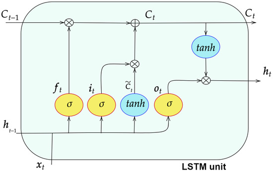
Figure 3. Architecture of the LSTM unit.

The process starts with the forget gate (see (9)), establishing which parts of the previous state can be considered irrelevant and therefore deleted. Consequently, it also determines the portion of information that will be retained for subsequent steps. The input gate (see (10)) selects the share of information that enters the internal state. In parallel, a tanh layer produces the candidate values ${\tilde{\mathit{C}}}_t$ (see (11)) to be integrated into the cell state together with ${\mathit{C}}_{t-1}$. At this point, the memory is updated as a linear combination of ${\mathit{C}}_{t-1}$ and ${\tilde{\mathit{C}}}_t$ through the weights ${\mathit{f}}_t$ and ${\mathit{i}}_t$, respectively, as stated in (12). Then, the output gate (see (13)) controls which part of the state ${\mathit{C}}_t$ should be returned. The final output of the LSTM layer, ${\mathit{h}}_t$, emerges from the interaction between ${\mathit{o}}_t$ and the cell state (see (14)), processed by a tanh function.

From a computational perspective, each LSTM unit involves the estimation of $4\times d_1\times (d_0+d_1+1)$ parameters. Indeed, for each subnet $k\in \{i,f,C,o\}$, there are: the input weights $W^{\left(k\right)}$ (dimensions $d_1\times d_0$), the hidden state weights $U^{\left(k\right)}$ (dimensions $d_1\times d_1$), and the bias term $b^{\left(k\right)}$ (dimensions $d_1\times 1$). Considering the four gates (input, forget, cell, and output), the total number of parameters grows accordingly.

A Multivariate Quantile-LSTM for CVaR Estimate

Following the approach proposed in [56], a multivariate quantile LSTM (q-LSTM) is designed to simultaneously estimate the CVaR at the $\alpha$ quantile for each asset in the portfolio. These estimates are subsequently provided as input for the computation of dissimilarities between each couple of assets, as stated in (4). As extensively discussed in [56], this choice is motivated by the lack of a closed-form solution when some strong assumptions—such as Gaussian distributions of returns and constant conditional correlations between each asset and the portfolio over time—do not hold.

Figure 4 illustrates the architecture of the q-LSTM model, which combines an LSTM unit with fully connected (FCN) layers.

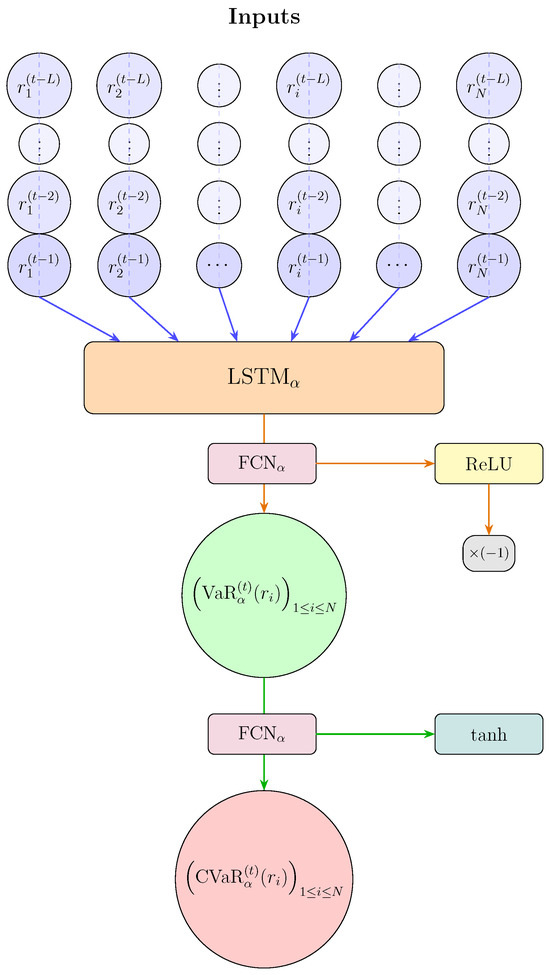
Figure 4. Diagram of the q-LSTM network for the CVaR estimation.

For each month t in the out-of-sample window, the LSTM unit (orange block) processes the time series of returns and generates a hidden state, represented by a latent vector. This vector serves as input to the branch responsible for the estimate of the distress quantile. The yellow block corresponds to the use of the ReLU activation function, while the blue block indicates the use of the tanh function. Initially, the LSTM output is fed into a fully connected layer (pink block) with a ReLU activation function, which produces the estimate of the Value-at-Risk at the $\alpha$ level for each asset (the green circle). Subsequently, the VaR values are passed as input to an additional fully connected layer with tanh activation, which yields the final output, i.e., the CVaR vector for the same quantile level $\alpha$. This architecture enables the joint modeling of multivariate VaR and CVaR, ensuring internal consistency between the two measures and reducing problems associated with the quantile crossing.

Denoted by $L\in \mathbb{N}$ a lookback period, we consider the lagged time series ${\mathit{r}}^{(t-\ell )}={\left(r_i^{(t-\ell )}\right)}_{1\le i\le N}$, for $\ell =1,\dots ,L$. The hidden state ${\mathit{h}}_{\alpha ,t}\in {\mathbb{R}}^{d_{\alpha }}$ (with $d_{\alpha }\in \mathbb{N}$), generated from the LSTM unit, is used to compute the VaR at the $\alpha$ quantile. Let ${\mathbf{VaR}}_{\alpha }^{\left(t\right)}={\left({\mathrm{VaR}}_{\alpha }^{\left(t\right)}\left(r_i\right)\right)}_{1\le i\le N}$ be defined as the vector of all VaR at the $\alpha$ quantile at time t, and it is given by

$${\mathbf{VaR}}_{\alpha }^{\left(t\right)}={\varphi }_{\alpha }^{\left(\mathrm{VaR}\right)}\left(W_{\alpha }^{\left(\mathrm{VaR}\right)}{\mathit{h}}_{\alpha ,t}+{\mathit{b}}_{\alpha }^{\left(\mathrm{VaR}\right)}\right)$$

(15)

where $W_{\alpha }^{\left(\mathrm{VaR}\right)}\in {\mathbb{R}}^{N\times d_{\alpha }}$ is the weight matrix, ${\mathit{b}}_{\alpha }^{\left(\mathrm{VaR}\right)}\in {\mathbb{R}}^N$ is the bias vector, and ${\varphi }_{\alpha }^{\left(\mathrm{VaR}\right)}$ is the ReLU activation function, applied with an ad hoc correction through the multiplication by $(-1)$. Subsequently, via an FCN layer, the ${\mathbf{CVaR}}_{\alpha }^{\left(t\right)}={\left({\mathrm{CVaR}}_{\alpha }^{\left(t\right)}\left(r_i\right)\right)}_{1\le i\le N}$ at time t is then generated as

$${\mathbf{CVaR}}_{\alpha }^{\left(t\right)}={\varphi }_{\alpha }^{\left(\mathrm{CVaR}\right)}\left(W_{\alpha }^{\left(\mathrm{CVaR}\right)}{\mathbf{VaR}}_{\alpha }^{\left(t\right)}+{\mathit{b}}_{\alpha }^{\left(\mathrm{CVaR}\right)}\right)$$

(16)

where $W_{\alpha }^{\left(\mathrm{CVaR}\right)}\in {\mathbb{R}}^{N\times N}$, ${\mathit{b}}_{\alpha }^{\left(\mathrm{CVaR}\right)}\in {\mathbb{R}}^N$, and ${\varphi }_{\alpha }^{\left(\mathrm{CVaR}\right)}$ is the tanh activation function.

The chosen hyperparameter configuration is summarized in Table 2 (see bottom side). Regarding the number of neurons per layer, after some preliminary tests, we set the value to $u_{\alpha }=50$ for the distress quantile. The dropout rate has been set to $10\%$ to prevent overfitting. This choice reflects that, for lower values of $\alpha$, the model can better capture extreme events. We set the batch size to 8 and the number of epochs to 500 for the VaR calculation. Since the architecture is integrated within an MOPSO framework, a limited number of epochs has been chosen to limit computational times. Empirical tests confirm that this configuration is adequate and avoids overfitting (see Appendix A).

Table 2. Parameter setting for the MOPSO solver and the LSTM architecture.

Parameter	Value
MOPSO solver
$N_{pop}$	600
$max\_iter$	500
$A_{max}$	200
$\omega$	0.4
$c_1$	2
$c_2$	2
$mu{t}_{\%}$	50%
LSTM architecture
$\alpha$	$0.05$
$u_{\alpha }$	50
dropoutα	$10\%$
batch-sizeα	8
epochsα	500
Activation Functions
${\mathrm{VaR}}_{\alpha }$	ReLU ×(−1)
${\mathrm{CVaR}}_{\alpha }$	tanh

The network parameters are estimated using the backpropagation (BP) algorithm. For quantile-based forecasts, CVaR is evaluated at the quantile level $\alpha =0.05$, as standard in the literature (see, e.g., [57]). Consistently, the pinball loss function is used, which measures the discrepancy between the $0.05$-quantile forecasts and the observed values. Weight optimization is performed via the Adam algorithm, particularly suited to deep learning because it dynamically adapts the learning rate based on the gradient’s first- and second-order moments. This adaptation allows for faster and more stable convergence, enabling the LSTM network to capture complex patterns in the data and minimize the loss function considered (see, e.g., [56] and references therein).

Remark 6. 

We remark that the inputs of the LSTM architecture are represented by the rate of returns, generated by the bootstrap technique, while the outputs are the CVaRs. Finally, the MOPSO algorithm designs the optimal weight allocation that solves the bi-objective optimization problem (1).

5. Experimental Results

In this section, we describe the parameter settings employed in the numerical analysis and present the efficient frontiers obtained month by month that show the best trade-offs between the augmented volatility and the portfolio diversification (see Section 5.1). Finally, we assess a profitability analysis for the efficient portfolio strategy that reaches the maximum Sharpe ratio for the three different sustainable-risk-aversion parameters $\lambda \in \{0,0.5,1\}$, for each dataset.

In Table 2, we introduce the parameter setting for the MOPSO solver and the LSTM architecture. Such a setting is based on some preliminary tests and is also coherent with the literature (see, e.g., [20,32,33,58]).

We recall that we employ an out-of-sample window, from January 2016 to December 2020, to point out the effects of the market changes on the behavior of the investments. Moreover, the in-sample window is represented by the period from January 2012 to December 2015, updated in each rebalancing phase. We execute the analysis on an Intel Core i5 with 8 GB RAM and a macOS 11.6.8 system using MATLAB R2025a.

5.1. Efficient Frontiers

We construct, for the three markets considered—Dow Jones Industrial, Euro Stoxx 50, and FTSE 100—the frontiers of efficient portfolios, i.e., the Pareto-efficient set of portfolios in the augmented volatility-diversification plane (we indicate the augmented volatility by $\sigma$). The frontiers are generated on the last day of December for each year in the out-of-sample window (2016–2020), and they are collected in Figure 5, distinguishing the cases according to the sustainable-risk-aversion parameter $\lambda$. We recall that $\lambda \in \{0,0.5,1\}$, corresponding, respectively, to sustainable (green frontier), balanced (blue frontier), and purely financial (black frontier) volatility cases.

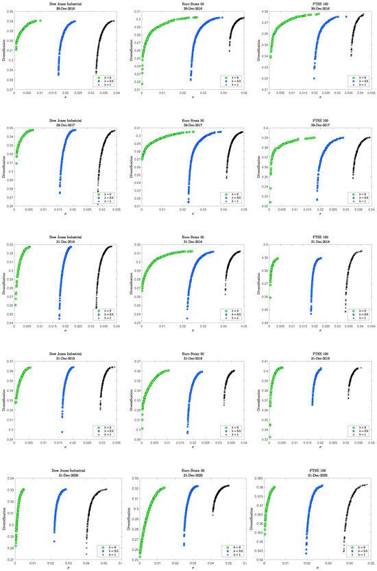
Figure 5. Efficient frontiers in the augmented volatility-diversification plane, for the three datasets on the last day of December for each year in the out-of-sample window—from 2016 (first row) to 2020 (last row). The x-axis reports the augmented volatility $\sigma$, i.e., $f_1\left(\mathbf{w}\right)$, while the y-axis represents the diversification index value, i.e., $f_2\left(\mathbf{w}\right)$. The colors indicate different levels of the sustainable-risk-aversion parameter.

The results reveal some interesting shared features. First, we can observe that over time, diversification requires a modest increase in volatility, especially for $\lambda =0$ and $\lambda =0.5$, as illustrated by vertical gaps on the left tails. This feature indicates that sustainable or balanced portfolios achieve better diversification without excessive risk costs. This behavior is repeated across the three different markets.

Looking at the differences among markets, as the number of assets increases, obtaining more diversified portfolios requires a more significant increase in volatility. This effect, once again, is more pronounced in the cases of $\lambda =0$ and $\lambda =0.5$, while it is attenuated for $\lambda =1$. This occurs because the introduction of the sustainability component in volatility encourages a more homogeneous distribution of portfolio weights. Graphically, this greater diversification appears as a longer right tail with horizontal gaps (see, for instance, Euro Stoxx 50 and FTSE 100 in 2016–2017).

Moreover, the black curves ($\lambda =1$), where only financial volatility is considered, show a steeper shape and a shift to the right. This shape suggests that, without an ESG component, diversification requires greater increases in pure risk. However, increasing the financial volatility tends to generate portfolios that are more concentrated compared with the other two cases.

Finally, we refer to Appendix B for a deeper analysis concerning the Pareto front outcomes and the optimal weight allocations. Specifically, we included an illustrative example where it should be noted that the optimal allocations are different depending on the sustainable-risk-aversion parameter.

5.2. Profitability Analysis

We consider a frictionless market in which no short selling is allowed, and all investors act as price takers. We indicate by ${\mathbf{w}}_t$ the optimal portfolio at the ex-post month t, with $t=1,\dots ,60$. The mean time of execution of each monthly rebalancing phase is reported in Table 3 for each dataset.

Table 3. Mean time of execution of each monthly allocation problem for each dataset.

Dataset Name	Computational Time (s)
Dow Jones Industrial	26.2567
Euro Stoxx 50	28.4240
FTSE 100	35.9011

Since the investment plan is time dependent, we assume an initial wealth $W_0=10,000,000$ (in each local currency) and we explicitly evaluate the magnitude of the trading through the cost function $c({\mathbf{w}}_t,{\mathbf{w}}_{t^{-}})$ introduced in [59]. In particular, concerning the transaction cost function, following [59], we considered the general complex structure that was offered by OCBC Securities, a broking firm in Singapore (www.iocbc.com), with five different trading segments, whose characteristics are reported in Table 4. For more details, we refer interested readers to Sections 3 and 5 of [59].

Table 4. Structure of transaction costs as in [59].

Trading Segment ${\mathit{t}}_{\mathit{s}}$ (Local Currency)	Fixed Fee (Local Currency)	Proportional Cost (%)
$0\le t_s\le 8000$	40	0
$8000<t_s\le 50,000$	0	0.5
$50,000<t_s\le 100,000$	0	0.4
$100,000<t_s\le 200,000$	0	0.25
$t_s>200,000$	400	0

5.3. Ex-Post Performance Measures

In this subsection, we present the ex-post measures considered to evaluate the profitability of the investment strategies with $\lambda \in \{0,0.5,1\}$. We denote by $r_{\mathbf{w},t}^{ex-post}$ the ex-post portfolio rate of return realized at time t, with $t=1,\dots ,60$. First of all, we introduce the so-called ex-post Sharpe ratio, defined as

$$SR={\displaystyle \frac{{\mu }^{ex-post}}{{\sigma }^{ex-post}}}$$

(17)

where ${\mu }^{ex-post}$ and ${\sigma }^{ex-post}$ are the mean and the standard deviation of the ex-post portfolio rates of return, respectively.

Further, to measure the profitability of the investment at time t, we compute the net wealth given by the following formula,

$$W_t=W_{t-1}\left(1+r_{\mathbf{w},t}^{ex-post}\right)-c({\mathbf{w}}_t,{\mathbf{w}}_{t^{-}}).$$

(18)

In the previous equation, ${\mathbf{w}}_{t^{-}}=(w_{t^{-},1},\dots ,w_{t^{-},N})$ represents the re-normalized portfolio weight before the rebalancing at time t (see [60]), which is defined for $t=2,\dots ,60$ as

$$w_{t^{-},i}={\displaystyle \frac{w_{t-1,i}{r}_{t-1,i}^{gross}}{{\sum }_{j=1}^N{w}_{t-1,j}{r}_{t-1,j}^{gross}}}$$

(19)

where the denominator is the gross portfolio return at month $t-1$. The gross return of asset i at month t is defined as $r_{t-1,i}^{\mathrm{gross}}={\displaystyle \frac{p_{i,t}}{p_{i,t-1}}}$, where $p_{i,t}$ is the price (adjusted for splits and dividends) of the i-th asset at the end of month t.

At time $t=1$, we set ${\mathbf{w}}_{t^{-}}=\mathbf{0}$.

In this way, the turnover is calculated as

$$TR=\sum _{i=1}^N|w_{t,i}-w_{t^{-},i}|.$$

(20)

Remark 7. 

According to the change in the portfolio weights between consecutive rebalancing periods, $w_{t,i}-w_{t^{-},i}$ represents the trades of rebalancing the i-th asset at time t. The changes in positions during each rebalancing period are related to the transaction costs.

In addition, we evaluate the so-called compound annual growth rate, calculated as

$$CAGR={\left({\displaystyle \frac{W_{60}}{W_0}}\right)}^{{\displaystyle \frac{12}{60}}}-1$$

(21)

where $W_0$ represents the initial wealth and $W_{60}$ is the final wealth of the last month.

At this point, in order to assess the capacity of a strategy to avoid high losses, we introduce the drawdown measure [61]

$$D{D}_t=min\left\{0,{\displaystyle \frac{W_t-W_{peak}}{W_{peak}}}\right\}$$

(22)

where $W_{peak}$ is the maximum amount of wealth reached by the strategy until time t. In particular, we consider the mean (mean DD), the standard deviation (std DD), and the maximum (max DD) of the drawdown measure over time.

Finally, to understand the ex-post portfolio diversification, we exploit the diversification index [62], defined as

$$DI=1-HI=1-\sum _{i=1}^N{w}_i^2$$

(23)

where $HI$ represents the Herfindahl Index.

5.4. Ex-Post Performance Analysis

In the ex-post analysis, we investigate the profitability of different allocation strategies concerning the agent’s sustainable-risk-aversion parameter $\lambda$. We recall that the selected efficient portfolio is the one that reaches the maximum Sharpe ratio on the Pareto front.

The empirical results are summarized in Table 5. We recall that for $\lambda =0$, the agent is completely sustainable-risk-adverse; if $\lambda =1$, one considers only the financial volatility, while for $\lambda =0.5$, there is a balance between the financial and sustainable volatilities.

Table 5. Ex-post performance measures of the proposed portfolio allocation model for different allocation strategies on the three datasets. The bold formatting indicates the significant values in the table to facilitate the reading of the results.

$\mathit{\lambda }$ Value	$\mathit{\lambda }=0$	$\mathit{\lambda }=0.5$	$\mathit{\lambda }=1$	EW
Dow Jones Industrial
CAGR	0.3151	0.2883	0.2966	0.1294
SR	0.5954	0.6127	0.6615	0.2716
${\mu }^{ex-post}$	0.0245	0.0226	0.0230	0.0113
${\sigma }^{ex-post}$	0.0413	0.0370	0.0349	0.0418
mean DD	−0.0121	−0.0109	−0.0100	−0.0247
std DD	0.0271	0.0243	0.0234	0.0405
max DD	−0.1359	−0.1114	−0.1097	−0.2039
TR	0.6584	0.6648	0.6378	–
IQRTR	0.3772	0.4964	0.4810	–
$c_{reb}$	8618.7	8393.5	7965.6	–
DI	0.7951	0.7983	0.8022	–
nnz assets (avg)	22	21	21	28
nnz assets (min)	12	11	13	28
Euro Stoxx 50
CAGR	0.3711	0.3300	0.2726	0.0671
SR	0.6201	0.6929	0.6207	0.1343
${\mu }^{ex-post}$	0.0283	0.0254	0.0215	0.0071
${\sigma }^{ex-post}$	0.0457	0.0367	0.0347	0.0533
mean DD	−0.0104	−0.0075	−0.0070	−0.0514
std DD	0.0283	0.0212	0.0168	0.0627
max DD	−0.1753	−0.1336	−0.1009	−0.2744
TR	0.7522	0.8165	0.6536	–
IQRTR	0.4175	0.6460	0.4758	–
$c_{reb}$	10343	9937.4	8174.1	–
DI	0.8552	0.8534	0.8461	–
nnz assets (avg)	30	30	27	45
nnz assets (min)	13	12	10	45
FTSE 100
CAGR	0.3101	0.2484	0.2447	0.0649
SR	0.5816	0.5839	0.5844	0.1517
${\mu }^{ex-post}$	0.0246	0.0202	0.0199	0.0066
${\sigma }^{ex-post}$	0.0423	0.0347	0.0341	0.0439
mean DD	−0.0151	−0.0113	−0.0098	−0.0464
std DD	0.0322	0.0236	0.0206	0.0678
max DD	−0.1636	−0.1276	−0.1139	−0.2634
TR	0.8893	0.8401	0.8099	–
IQRTR	0.3752	0.3349	0.4565	–
$c_{reb}$	15502	15022	13627	–
DI	0.9380	0.9518	0.9490	–
nnz assets (avg)	56	54	51	80
nnz assets (min)	19	20	18	80

Such a table shows the results for the ex-post performance measures presented in the previous Section 5.3 for the three different levels of $\lambda \in \{0,0.5,1\}$ and for the three different datasets. Moreover, we compare such strategies with the traditional Equally Weighted (EW) portfolio allocation strategy (see [63]). Specifically, the last two rows, nnz assets (avg) and nnz assets (min), indicate, respectively, the average (it is worth underlining that the average number is rounded to the lower integer) and the minimum number of non-zero assets across the 60 out-of-sample months. In addition, $c_{reb}$ represents the costs due to the rebalancing phases, calculated via the Table 4.

Finally, in Figure 6 we present the net wealth trend for all the datasets.

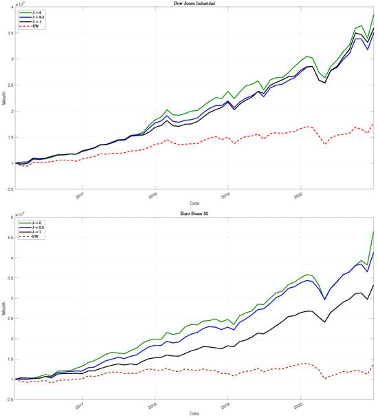
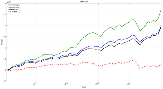
Figure 6. Evolution of the net wealth for the three different $\lambda$ levels and the Equally Weighted (EW) allocation, using the assets in the three datasets.

Remark 8. 

It is worth mentioning that the allocation strategies presented are active investing and not index-linked strategies.

In general, from the results of Table 5, we can infer that strategies with $\lambda =0$ have higher profits but result in higher volatility values. The balanced strategy with $\lambda =0.5$ shows better profit/risk trade-offs, presenting higher Sharpe ratio measures and generally higher diversification benefits. Finally, allocations with $\lambda =1$ present lower overall portfolio risk. In particular, one has lower risk measures (standard deviation and drawdown). As a consequence, the turnover is better controlled as well as the rebalancing costs. The results are preserved for all three datasets, although they are more pronounced as the number of assets increases. Regarding stability, the interquartile ranges of turnover (IQRs_TR) indicate the lowest dispersion at $\lambda =0$ for the Dow Jones Industrial and Euro Stoxx 50, and at $\lambda =0.5$ for the FTSE 100, confirming that turnover stability is dataset-specific.

The previous analysis could be justified considering that the financial volatility seems to be heavier than the sustainable one, and it influences the allocation process.

In any case, the introduction of the volatility information gives good results, showing a balanced strategy (with $\lambda =0.5$) for a moderate agent who looks for a trade-off between profit and risk in the different cases analyzed, taking into account the diversification benefits.

Such an analysis is graphically corroborated by the findings in Figure 6.

Remark 9. 

It is worth stressing that all the strategies proposed outperform the Equally Weighted (EW) portfolio allocation.

6. Conclusions and Future Works

In this paper, we tackled a bi-objective optimization problem in which we aim to maximize the portfolio diversification and, at the same time, minimize the augmented portfolio volatility, where the ESG information is incorporated. Moreover, we developed an improved MOPSO embedded with a repair-and-projection mechanism to satisfy the constraints, and we implemented a deep learning architecture to improve the quality of estimating the portfolio diversification goal. Finally, we conducted empirical tests on datasets from three different countries’ markets to illustrate the effectiveness of the proposed strategies, accounting for various sustainable-risk-aversion appetites.

For future work, we plan to extend the bi-objective paradigm to a tri-objective framework where a profit measure is incorporated in the optimization process. Furthermore, we would also like to develop suitable constraint-handling techniques to keep the transaction costs under control. Finally, another interesting direction might be to examine how the results vary across the three different markets when exchange-rate effects are taken into account and to explore the use of the proposed methodology for hedging purposes.

References

- Hagin, R.L. Investment Management: Portfolio Diversification, Risk, and Timing–Fact and Fiction; John Wiley & Sons: Hoboken, NJ, USA, 2004; Volume 235. [Google Scholar]
- Markowitz, H. Modern portfolio theory. J. Financ. 1952, 7, 77–91. [Google Scholar]
- Koumou, G.B. Diversification and portfolio theory: A review. Financ. Mark. Portf. Manag. 2020, 34, 267–312. [Google Scholar] [CrossRef]
- Meucci, A. Managing diversification. Risk 2009, 22, 74–79. [Google Scholar]
- Pola, G. On entropy and portfolio diversification. J. Asset Manag. 2016, 17, 218–228. [Google Scholar] [CrossRef]
- Ararat, Ç.; Cesarone, F.; Pınar, M.Ç.; Ricci, J.M. MAD risk parity portfolios. Ann. Oper. Res. 2024, 336, 899–924. [Google Scholar] [CrossRef]
- Hoepner, A.G. Corporate Social Responsibility and Investment Portfolio Diversification. 2010. Available online: https://papers.ssrn.com/sol3/papers.cfm?abstract_id=1599334 (accessed on 11 August 2025).
- Sbaiz, G. Sustainable information into portfolio optimization models. J. Appliedmath 2023, 1, 125. [Google Scholar] [CrossRef]
- Brauers, W.K. Optimization Methods for a Stakeholder Society: A Revolution in Economic Thinking by Multi-Objective Optimization; Springer Science & Business Media: Berlin/Heidelberg, Germany, 2003; Volume 73. [Google Scholar]
- Coello, C.A.C. Evolutionary multi-objective optimization in finance. In Handbook of Research on Nature-Inspired Computing for Economics and Management; IGI Global: Hershey, PA, USA, 2007; pp. 74–89. [Google Scholar]
- Doumpos, M.; Zopounidis, C. Multi-objective optimization models in finance and investments. J. Glob. Optim. 2020, 76, 243–244. [Google Scholar] [CrossRef]
- Fabretti, A.; Herzel, S. Delegated portfolio management with socially responsible investment constraints. Eur. J. Financ. 2012, 18, 293–309. [Google Scholar] [CrossRef]
- Utz, S.; Wimmer, M.; Hirschberger, M.; Steuer, R.E. Tri-criterion inverse portfolio optimization with application to socially responsible mutual funds. Eur. J. Oper. Res. 2014, 234, 491–498. [Google Scholar] [CrossRef]
- Coqueret, G. Diversified minimum-variance portfolios. Ann. Financ. 2015, 11, 221–241. [Google Scholar] [CrossRef]
- Gasser, S.M.; Rammerstorfer, M.; Weinmayer, K. Markowitz revisited: Social portfolio engineering. Eur. J. Oper. Res. 2017, 258, 1181–1190. [Google Scholar] [CrossRef]
- Pedersen, L.H.; Fitzgibbons, S.; Pomorski, L. Responsible investing: The ESG-efficient frontier. J. Financ. Econ. 2021, 142, 572–597. [Google Scholar] [CrossRef]
- Steuer, R.E.; Utz, S. Non-contour efficient fronts for identifying most preferred portfolios in sustainability investing. Eur. J. Oper. Res. 2023, 306, 742–753. [Google Scholar] [CrossRef]
- Ling, A.; Li, J.; Wen, L.; Zhang, Y. When trackers are aware of ESG: Do ESG ratings matter to tracking error portfolio performance? Econ. Model. 2023, 125, 106346. [Google Scholar] [CrossRef]
- Carmichael, B.; Koumou, G.B.; Moran, K. Unifying portfolio diversification measures using Rao’s quadratic entropy. J. Quant. Econ. 2023, 21, 769–802. [Google Scholar] [CrossRef]
- Aprea, I.L.; Sbaiz, G. A neural network-particle swarm solver for sustainable portfolio optimization problems. In Decisions in Economics and Finance; Springer: Berlin/Heidelberg, Germany, 2025; pp. 1–40. [Google Scholar]
- Zeidan, R.; Onabolu, S. The generalized sustainability credit rating system. Braz. Rev. Financ. 2023, 21, 21–47. [Google Scholar] [CrossRef]
- Poveda, C.A.; Lipsett, M.G. A review of sustainability assessment and sustainability/environmental rating systems and credit weighting tools. J. Sustain. Dev. 2011, 4, 36. [Google Scholar] [CrossRef]
- Zeidan, R.; Boechat, C.; Fleury, A. Developing a sustainability credit score system. J. Bus. Ethics 2015, 127, 283–296. [Google Scholar] [CrossRef]
- Gutiérrez-Nieto, B.; Serrano-Cinca, C.; Camón-Cala, J. A credit score system for socially responsible lending. J. Bus. Ethics 2016, 133, 691–701. [Google Scholar] [CrossRef]
- Kennedy, J.; Eberhart, R. Particle swarm optimization. In Proceedings of the ICNN’95-International Conference on Neural Networks, Perth, WA, Australia, 27 November–1 December 1995; Volume 4, pp. 1942–1948. [Google Scholar]
- Mostaghim, S.; Teich, J. Strategies for finding good local guides in multi-objective particle swarm optimization (MOPSO). In Proceedings of the 2003 IEEE Swarm Intelligence Symposium. SIS’03 (Cat. No. 03EX706), Indianapolis, IN, USA, 26–26 April 2003; pp. 26–33. [Google Scholar]
- Zheng, X.; Liu, H. A hybrid vertical mutation and self-adaptation based MOPSO. Comput. Math. Appl. 2009, 57, 2030–2038. [Google Scholar] [CrossRef]
- Lalwani, S.; Singhal, S.; Kumar, R.; Gupta, N. A comprehensive survey: Applications of multi-objective particle swarm optimization (MOPSO) algorithm. Trans. Comb. 2013, 2, 39–101. [Google Scholar]
- Sun, Y.; Gao, Y. A multi-objective particle swarm optimization algorithm based on gaussian mutation and an improved learning strategy. Mathematics 2019, 7, 148. [Google Scholar] [CrossRef]
- Chen, J.; Liu, Y.; Luo, Y.; Ouyang, A.; Yang, J.; Bai, W. Multi-objective particle swarm optimization algorithm for task allocation and archived guided mutation strategies. Sci. Rep. 2025, 15, 15821. [Google Scholar] [CrossRef] [PubMed]
- Moore, J. Application of Particle Swarm to Multiobjective Optimization. Technical Report. 1999. Available online: https://cir.nii.ac.jp/crid/1571980076089705344 (accessed on 11 August 2025).
- Coello, C.A.C.; Pulido, G.T.; Lechuga, M.S. Handling multiple objectives with particle swarm optimization. IEEE Trans. Evol. Comput. 2004, 8, 256–279. [Google Scholar] [CrossRef]
- Sierra, M.R.; Coello Coello, C.A. Improving PSO-based multi-objective optimization using crowding, mutation and ϵ-dominance. In Proceedings of the International Conference on Evolutionary Multi-Criterion Optimization, Guanajuato, Mexico, 9–11 March 2005; Springer: Berlin/Heidelberg, Germany, 2005; pp. 505–519. [Google Scholar]
- Durillo, J.J.; García-Nieto, J.; Nebro, A.J.; Coello, C.A.C.; Luna, F.; Alba, E. Multi-objective particle swarm optimizers: An experimental comparison. In Proceedings of the Evolutionary Multi-Criterion Optimization: 5th International Conference, EMO 2009, Nantes, France, 7–10 April 2009; Springer: Berlin/Heidelberg, Germany, 2009; pp. 495–509. [Google Scholar]
- Reyes-Sierra, M.; Coello, C.C. Multi-objective particle swarm optimizers: A survey of the state-of-the-art. Int. J. Comput. Intell. Res. 2006, 2, 287–308. [Google Scholar] [CrossRef]
- Chalvatzis, C.; Hristu-Varsakelis, D. High-performance stock index trading via neural networks and trees. Appl. Soft Comput. 2020, 96, 106567. [Google Scholar] [CrossRef]
- Heaton, J.B.; Polson, N.G.; Witte, J.H. Deep learning for finance: Deep portfolios. Appl. Stoch. Model. Bus. Ind. 2017, 33, 3–12. [Google Scholar] [CrossRef]
- Garcia-Garcia, A.; Orts-Escolano, S.; Oprea, S.; Villena-Martinez, V.; Martinez-Gonzalez, P.; Garcia-Rodriguez, J. A survey on deep learning techniques for image and video semantic segmentation. Appl. Soft Comput. 2018, 70, 41–65. [Google Scholar] [CrossRef]
- Nassif, A.B.; Elnagar, A.; Shahin, I.; Henno, S. Deep learning for Arabic subjective sentiment analysis: Challenges and research opportunities. Appl. Soft Comput. 2021, 98, 106836. [Google Scholar] [CrossRef]
- Rosenblatt, F. The perceptron: A probabilistic model for information storage and organization in the brain. Psychol. Rev. 1958, 65, 386. [Google Scholar] [CrossRef]
- Elman, J.L. Finding structure in time. Cogn. Sci. 1990, 14, 179–211. [Google Scholar] [CrossRef]
- Hochreiter, S.; Schmidhuber, J. Long short-term memory. Neural Comput. 1997, 9, 1735–1780. [Google Scholar] [CrossRef] [PubMed]
- Md, A.Q.; Kapoor, S.; AV, C.J.; Sivaraman, A.K.; Tee, K.F.; Sabireen, H.; Janakiraman, N. Novel optimization approach for stock price forecasting using multi-layered sequential LSTM. Appl. Soft Comput. 2022, 134, 109830. [Google Scholar] [CrossRef]
- Cho, K.; Van Merriënboer, B.; Bahdanau, D.; Bengio, Y. On the properties of neural machine translation: Encoder-decoder approaches. arXiv 2014, arXiv:1409.1259. [Google Scholar] [CrossRef]
- Aslan, A.; Posch, P.N. How do investors value sustainability? A utility-based preference optimization. Sustainability 2022, 14, 15963. [Google Scholar] [CrossRef]
- Dorfleitner, G.; Utz, S. Safety first portfolio choice based on financial and sustainability returns. Eur. J. Oper. Res. 2012, 221, 155–164. [Google Scholar] [CrossRef]
- Borra, S.; Hill, A.D.C.M. Statistica-Metodologie per le Scienze Economiche e Sociali/2e; McGraw-Hill: New York, NY, USA, 2014. [Google Scholar]
- Rockafellar, R.T.; Uryasev, S. Optimization of conditional value-at-risk. J. Risk 2000, 2, 21–42. [Google Scholar] [CrossRef]
- Leitner, J. A short note on second-order stochastic dominance preserving coherent risk measures. Math. Financ. Int. J. Math. Stat. Financ. Econ. 2005, 15, 649–651. [Google Scholar] [CrossRef]
- Cesarone, F.; Martino, M.L.; Carleo, A. Does ESG impact really enhance portfolio profitability? Sustainability 2022, 14, 2050. [Google Scholar] [CrossRef]
- Politis, D.N.; Romano, J.P. The stationary bootstrap. J. Am. Stat. Assoc. 1994, 89, 1303–1313. [Google Scholar] [CrossRef]
- Politis, D.N.; White, H. Automatic block-length selection for the dependent bootstrap. Econom. Rev. 2004, 23, 53–70. [Google Scholar] [CrossRef]
- Ledoit, O.; Wolf, M. Honey, I shrunk the sample covariance matrix. J. Portf. Manag. 2004, 30, 110–119. [Google Scholar] [CrossRef]
- Beck, A. First-Order Methods in Optimization; SIAM: Philadelphia, PA, USA, 2017. [Google Scholar]
- Meghwani, S.S.; Thakur, M. Multi–criteria algorithms for portfolio optimization under practical constraints. Swarm Evol. Comput. 2017, 37, 104–125. [Google Scholar] [CrossRef]
- Aprea, I.L.; Scognamiglio, S.; Zanetti, P. Systemic risk measurement: A quantile long short-term memory network approach. Appl. Soft Comput. 2024, 152, 111224. [Google Scholar] [CrossRef]
- Tobias, A.; Brunnermeier, M.K. CoVaR. Am. Econ. Rev. 2016, 106, 1705. [Google Scholar] [CrossRef]
- Goodfellow, I.; Bengio, Y.; Courville, A.; Bengio, Y. Deep Learning; MIT Press Cambridge: Cambridge, MA, USA, 2016; Volume 1. [Google Scholar]
- Beraldi, P.; Violi, A.; Ferrara, M.; Ciancio, C.; Pansera, B.A. Dealing with complex transaction costs in portfolio management. Ann. Oper. Res. 2021, 299, 7–22. [Google Scholar] [CrossRef]
- Shen, W.; Wang, J.; Ma, S. Doubly regularized portfolio with risk minimization. In Proceedings of the AAAI Conference on Artificial Intelligence, Québec City, QC, Canada, 27–31 July 2014; Volume 28. [Google Scholar]
- Chekhlov, A.; Uryasev, S.; Zabarankin, M. Drawdown measure in portfolio optimization. Int. J. Theor. Appl. Financ. 2005, 8, 13–58. [Google Scholar] [CrossRef]
- Woerheide, W.; Persson, D. An index of portfolio diversification. Financ. Serv. Rev. 1992, 2, 73–85. [Google Scholar] [CrossRef]
- DeMiguel, V.; Garlappi, L.; Uppal, R. Optimal versus naive diversification: How inefficient is the 1/N portfolio strategy? Rev. Financ. Stud. 2009, 22, 1915–1953. [Google Scholar] [CrossRef]
- Schott, J.R. Fault Tolerant Design Using Single and Multicriteria Genetic Algorithm Optimization. Master’s Thesis, Massachusetts Institute of Technology, Cambridge, MA, USA, 1995. [Google Scholar]
- Wang, Y.N.; Wu, L.H.; Yuan, X.F. Multi-objective self-adaptive differential evolution with elitist archive and crowding entropy-based diversity measure. Soft Comput. 2010, 14, 193–209. [Google Scholar] [CrossRef]
Disclaimer/Publisher’s Note: The statements, opinions and data contained in all publications are solely those of the individual author(s) and contributor(s) and not of MDPI and/or the editor(s). MDPI and/or the editor(s) disclaim responsibility for any injury to people or property resulting from any ideas, methods, instructions or products referred to in the content. |
© 2025 by the authors. Licensee MDPI, Basel, Switzerland. This article is an open access article distributed under the terms and conditions of the Creative Commons Attribution (CC BY) license (https://creativecommons.org/licenses/by/4.0/).