Deep Learning-Based Back-Projection Parameter Estimation for Quantitative Defect Assessment in Single-Framed Endoscopic Imaging of Water Pipelines

Abstract

Aging water pipelines are increasingly prone to structural failure, leakage, and ground subsidence, creating critical risks to urban infrastructure. Closed-circuit television endoscopy is widely used for internal assessment, but it depends on manual interpretation and lacks reliable quantitative defect information. Traditional vanishing point detection techniques, such as the Hough Transform, often fail under practical conditions due to irregular lighting, debris, and deformed pipe surfaces, especially when pipes are water-filled. To overcome these challenges, this study introduces a deep learning-based method that estimates inverse projection parameters from monocular endoscopic images. The proposed approach reconstructs a spatially accurate two-dimensional projection of the pipe interior from a single frame, enabling defect quantification for cracks, scaling, and delamination. This eliminates the need for stereo cameras or additional sensors, providing a robust and cost-effective solution compatible with existing inspection systems. By integrating convolutional neural networks with geometric projection estimation, the framework advances computational intelligence applications in pipeline condition monitoring. Experimental validation demonstrates high accuracy in pose estimation and defect size recovery, confirming the potential of the system for automated, non-disruptive pipeline health evaluation.

1. Introduction

Water pipelines are one of the most critical infrastructures in urban water supply systems, as they ensure the safe delivery of hygienic and pressurized drinking water to end-users in sufficient quantities. In response to rising urban population density and water demand, these pipelines were installed in large numbers, primarily in the 1980s. Consequently, a significant portion of the pipeline infrastructure has entered a stage of severe aging. According to recent statistics, pipelines older than 21 years comprise approximately 93,969 km, accounting for 38.2% of the total network; when including pipelines aged 16–20 years, this proportion exceeds 50% [1]. However, the annual replacement and rehabilitation rates remain at only 0.3% and 0.4%, respectively, leading to a steady increase in the proportion of aged pipelines. Over time, aging pipelines accumulate structural degradation owing to a combination of external environmental factors (e.g., groundwater infiltration, freezing, and vibration) and internal operational stress (e.g., pressure fluctuation and flow of foreign matter). This results in a significantly higher failure rate compared to newer pipelines, causing increased occurrences of water outages, repeated maintenance costs, and water loss, ultimately imposing direct inconvenience to consumers [2,3]. Furthermore, because most water pipelines are buried underground, early visual inspection and preventive diagnosis are difficult. Failures typically become evident only after damage has already occurred. Leaks caused by pipe failures not only reduce pressure and wastewater but can also lead to secondary damage, such as soil erosion, void formation, and ground subsidence [4,5,6,7], occasionally escalating to road collapse or life-threatening incidents.

Periodic condition assessments are essential to prevent such risks and ensure sustainable asset management of urban water networks [8]. Modern asset management systems evaluate pipelines throughout their lifecycle to make informed decisions regarding maintenance, repair, or replacement. These assessments are classified into indirect and direct methods. Indirect assessment estimates pipe aging using data such as the pipe material, installation year, corrosion environment, and maintenance history. When high-risk segments are identified, a direct inspection is performed. Direct assessment involves physical or visual inspection using various techniques such as optical (CCTV, laser scan), electromagnetic (magnetic flux leakage and remote field eddy current), and acoustic methods (sonar, Sahara, etc.) [9,10,11].

Among these, closed-circuit television (CCTV) inspection is the most widely adopted because of its cost-effectiveness and applicability to various pipe environments [12,13]. However, this method relies heavily on manual analysis and requires significant time and labor to interpret large amounts of video footage. These results are often subject to analyst biases and inconsistencies. Moreover, lens distortion, lighting variation, and perspective effects can distort the shape and size of defects, thereby reducing the assessment accuracy.

To overcome these limitations, recent studies have explored the application of deep-learning-based image analysis for defect detection and classification [14,15,16,17,18,19]. Techniques such as object detection using YOLO, CNN-based classification, and segmentation-based shape analysis have been used to automatically identify defects, such as cracks, scaling, and delamination [20,21,22]. These approaches have contributed to improved accuracy, reduced analysis time, and enhanced data-driven management systems [23,24]. Nevertheless, most existing deep learning models are trained on data collected in static and controlled environments. In real-world pipeline inspection scenarios, particularly under fully filled pipe (full-water) conditions, the models often face challenges such as uneven illumination, image blurring caused by internal contamination, and ambiguous defect boundaries. Additionally, many methods are limited to qualitative assessments and cannot recover the 3D spatial information required for accurate defect sizing.

The vanishing point within a pipeline image is a key element in a quantitative assessment. This is crucial for estimating the geometric orientation of the camera and enables the reconstruction of planar images via back-projection for spatial measurement. The Hough Transform has been traditionally employed to estimate vanishing points by detecting linear patterns in pipe wall textures or joint lines [25,26,27,28,29]. However, in practice, the accuracy of line detection is significantly reduced by uneven lighting and contamination, resulting in unreliable vanishing point estimations. Furthermore, for flexible or non-circular pipes, the assumption of geometric regularity no longer holds, rendering the method inapplicable [26,29].

Therefore, this paper proposes a novel computational intelligence method for estimating the back-projection parameters of monocular endoscopic images without the need for additional sensors. The proposed AI-based back-projection parameter estimation method reconstructs a spatially accurate planar image of the water pipeline interior using only a single frame. This reconstructed image enables the quantitative evaluation of internal defects, such as cracks, scaling, and peeling, providing a consistent and objective analysis. A major advantage of this approach is its sensor-free applicability in existing non-disruptive endoscopic systems. By leveraging AI to estimate the pose of the camera (i.e., back-projection parameters) with high precision, this method provides quantitative 2D spatial information and offers a new paradigm for automated, standardized, and digitized pipeline condition monitoring. Finally, this study establishes a technical foundation for transforming water infrastructure maintenance through objective and quantitative defect evaluation.

2. AI-Based Back-Projection Parameter Estimation for Quantitative Assessment of Internal Defects in Water Pipelines

In this study, an AI-based methodology is proposed to estimate the back-projection parameters necessary for the quantitative evaluation of internal defects within water pipelines using monocular endoscopic inspection images. The complete procedural flow is illustrated in Figure 1.

As an initial step, a dedicated annotation toolkit was developed to manually label key geometric features such as vanishing points and pipeline centerlines from images captured inside the pipeline. These features serve as foundational references for estimating the spatial position and orientation of the camera. Based on the annotated data, a training dataset was constructed for monocular internal inspection. An AI model was subsequently trained to perform regression of the back-projection parameters using a single video frame as the input. The effectiveness of the estimated back-projection was validated by assessing whether the quantitative measurements of the defects projected onto the reference image surface were consistent with the actual physical dimensions of the reference markers embedded in the environment.

2.1. Analysis of the Relationship Between Back-Projection Parameters and Image Features

The methodology relies on a back-projection approach, whereby 2D image coordinates are transformed back into their corresponding positions in 3D space. This transformation is critical for reconstructing the three-dimensional geometric structure of the internal surface of a water pipeline and for accurately measuring the location and size of the detected internal defects. Accurate back-projection depends on the precise estimation of the camera’s extrinsic parameters, which define the camera’s spatial position and orientation at the time of image acquisition. To this end, a mathematical relationship between the observable image features and extrinsic parameters was first derived to enable learning-based regression of these parameters using only a single frame from a monocular camera.

The imaging process is modeled using a pinhole camera configuration, which mathematically defines the projection of a 3D point onto a 2D image plane via the following projection matrix, as shown in Equation (1) [30]:

$$w·\left[\begin{array}{c}x\\ y\\ 1\end{array}\right]=K·R|t·\left[\begin{array}{c}r·\mathrm{c}\mathrm{o}\mathrm{s}\left(\phi \right)\\ r·\mathrm{s}\mathrm{i}\mathrm{n}\left(\phi \right)\\ \begin{array}{c}Z\\ 1\end{array}\end{array}\right]$$

(1)

$$K=\left[\begin{array}{ccc}{f}_x& 0& c_x\\ 0& f_y& c_y\\ 0& 0& 1\end{array}\right]$$

(2)

$$R|t=\left[\begin{array}{ccc}{r}_{11}& r_{12}& \begin{array}{cc}{r}_{13}& t_x\end{array}\\ r_{21}& r_{22}& \begin{array}{cc}{r}_{23}& t_y\end{array}\\ r_{31}& r_{32}& \begin{array}{cc}{r}_{33}& t_z\end{array}\end{array}\right]=\left.R_z·R_x·R_y\right|t$$

(3)

where K, the intrinsic parameter matrix, includes the focal lengths (fₓ, fᵧ) and optical center (cₓ, cᵧ). [R | t] represents the extrinsic parameters, consisting of a rotation matrix R and translation vector t. Moreover, the 3D coordinate point [X, Y, Z] resides on the internal cylindrical surface of the pipeline and is parameterized in terms of radius r and angular coordinate φ. Scalar w denotes the homogeneous scale factor in projective space.

Owing to the inherent rotational symmetry of cylindrical water pipelines, certain transformations, specifically camera roll (rotation about the Z-axis) and translation along the Z-axis, do not alter the projection results. Consequently, the estimation of back-projection parameters is limited to four key extrinsic variables: tₓ, tᵧ, θₓ (rotation about the X-axis), and θᵧ (rotation about the Y-axis).

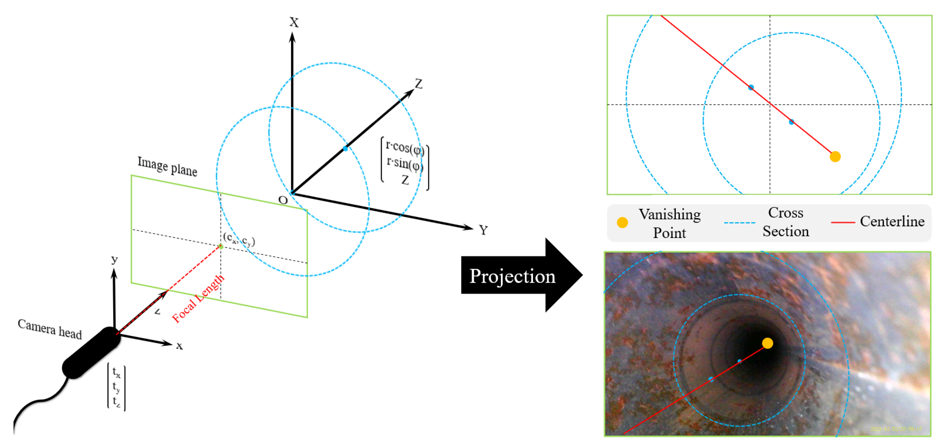
Several image features were extracted and analyzed to facilitate the estimation of these parameters, as illustrated in Figure 2. These include vanishing points (internal circular cross-sections that appear to converge owing to perspective), centerlines (representing virtual linear paths connecting cross-sectional centers along the pipeline), and illumination patterns (induced by onboard light sources, which vary with distance and orientation).

By eliminating the projection-invariant parameters (Z-axis rotation and translation), a reduced mathematical model was derived to quantify the correlation between observable image features and the remaining four extrinsic parameters. When rotation about the Y-axis (θᵧ) and translation along the X and Y axes (tₓ, tᵧ) are considered, the transformation of a 3D point into image coordinates can be approximated using Equation (4):

$$\left[\begin{array}{c}{X}^{\prime }\\ Y^{\prime }\\ Z^{\prime }\end{array}\right]=\left[\begin{array}{ccc}\mathrm{c}\mathrm{o}\mathrm{s}\left({\theta }_y\right)& 0& \mathrm{s}\mathrm{i}\mathrm{n}\left({\theta }_y\right)\\ 0& 1& 0\\ -\mathrm{s}\mathrm{i}\mathrm{n}\left({\theta }_y\right)& 0& \mathrm{c}\mathrm{o}\mathrm{s}\left({\theta }_y\right)\end{array} \begin{array}{c}{t}_x\\ t_y\\ 0\end{array}\right]\left[\begin{array}{c}r·\mathrm{c}\mathrm{o}\mathrm{s}\left(\phi \right)\\ r·\mathrm{s}\mathrm{i}\mathrm{n}\left(\phi \right)\\ \begin{array}{c}Z\\ 1\end{array}\end{array}\right]=\left[\begin{array}{c}r·\cos \left(\phi \right)·\cos \left({\theta }_y\right)+Z·\sin \left({\theta }_y\right)+t_x\\ r·\mathrm{s}\mathrm{i}\mathrm{n}\left(\phi \right)+t_y\\ -r·\cos \left(\phi \right)·\sin \left({\theta }_y\right)+Z·\cos \left({\theta }_y\right)\end{array}\right]$$

(4)

From this relationship, the vanishing point along the X-axis can be derived by taking the limit as Z → ∞, as in Equations (5) and (6):

$$Vanishing Poin{t}_x=\underset{Z\to \infty }{\lim }{\displaystyle \frac{f_x{·X}^{\prime }+c_x{Z}^{\prime }}{Z^{\prime }}}=\underset{Z\to \infty }{\lim }{\displaystyle \frac{f_x·Z·\sin \left({\theta }_y\right)+c_{x}Z·\cos \left({\theta }_y\right)}{Z·\cos \left({\theta }_y\right)}}=f_x·\tan \left({\theta }_y\right)+c_x$$

(5)

Similarly, for rotation about the X-axis, the Y-coordinate of the vanishing point is given by

$$Vanishing Poin{t}_y=f_y·\tan \left({\theta }_x\right)+c_y$$

(6)

This mathematical formulation demonstrates that the horizontal position of the vanishing point is influenced by the Y-axis rotation angle, whereas the vertical position is determined by the X-axis rotation angle. The evolution of the location of the vanishing point in response to these rotational variations is shown in Figure 3.

In addition, the projection of a virtual pipeline centerline, represented as [0, 0, Z, 1]^T and subjected to camera translation and rotation, can be expressed as a function of Z in Equation (7).

$$\left[\begin{array}{c}x\left(Z\right)\\ y\left(Z\right)\\ 1\end{array}\right]=\left[\begin{array}{c}{\displaystyle \frac{f_x(Zsin\left({\theta }_y\right)\cos \left({\theta }_x\right)+t_x)}{Zcos\left({\theta }_y\right)\mathrm{c}\mathrm{o}\mathrm{s}\left({\theta }_x\right)}}+c_x\\ -{\displaystyle \frac{f_y(Zsin\left({\theta }_x\right)+t_y)}{Zcos\left({\theta }_y\right)\mathrm{c}\mathrm{o}\mathrm{s}\left({\theta }_x\right)}}+c_y\\ 1\end{array}\right]$$

(7)

The deviation in the projected centerline from the vanishing point is quantified by displacement vectors Δx(Z) and Δy(Z), computed as differences from Equations (5) and (6), as given in Equation (8):

$$\left\{\begin{array}{c}∆x\left(Z\right)\\ ∆y\left(Z\right)\end{array}\right.=\left\{\begin{array}{c}{\displaystyle \frac{f_x{t}_x}{Zcos\left({\theta }_y\right)\mathrm{c}\mathrm{o}\mathrm{s}\left({\theta }_x\right)}}\\ -{\displaystyle \frac{f_y{t}_y}{Zcos\left({\theta }_y\right)\mathrm{c}\mathrm{o}\mathrm{s}\left({\theta }_x\right)}}\end{array}\right.$$

(8)

Assuming fₓ = fᵧ, the displacement vectors define a slope θ corresponding to the angle of the projected centerline, and the translation components can be rewritten using trigonometric relationships in Equations (9) and (10):

$$t_x=-\cos \left(\theta \right)\sqrt{t_x^2+t_y^2}$$

(9)

$$t_y=-\mathit{sin}\left(\theta \right)\sqrt{t_x^2+t_y^2}$$

(10)

Furthermore, the total displacement magnitude √(tₓ² + tᵧ²) can be parameterized in terms of the pipeline’s physical radius r and the geometric ratio G_ratio, derived from observed cross-sectional deformation patterns in Equations (11) and (12):

$$t_x=-\cos \left(\theta \right)·r·G_{ratio}$$

(11)

$$t_y=-\mathit{sin}\left(\theta \right)·r·G_{ratio}$$

(12)

These equations collectively establish the foundational relationship between the observable features in monocular inspection images and the external parameters necessary for back-projection. They enable the robust estimation of camera poses, even from a single frame, thereby supporting the accurate and automated quantification of internal defects in water pipeline systems.

2.2. Endoscopic Inspection Data

A combination of previously collected in-service (non-disruptive) pipeline inspection videos and newly captured experimental footage was used to construct a dataset suitable for training AI models aimed at estimating back-projection parameters from monocular endoscopic inspection images. The experimental setup included pipelines fabricated from various materials commonly used in both operational and degraded water distribution systems, including cast iron, polyethylene, steel, and polyvinyl chloride. Additionally, mock-defect environments were created using 3D-printed pipelines and paper-based cylindrical models. These diverse conditions were selected to ensure robustness across a wide range of pipeline types and inspection scenarios.

The diameter specifications of each pipe type used in the experiment are listed in

Table 1. Pipe types and diameters used in the experiments.

Type	Steel Pipe (SP)	Polyvinyl Chloride Pipe (PVC)	3D Printing Pipe	Paper Pipe (PP)	Cost Iron Pipe (CIP)	Polyethylene Pipe (PE)
Diameter (mm)	23	84, 116	84	34	86, 150	52

. The video data were recorded using a monocular endoscopic camera at various imaging resolutions: Full HD (1920 × 1080), HD (1280 × 720), and SD (720 × 480). The frames were captured under randomized camera poses to reflect diverse inspection conditions. Furthermore, both water-filled and empty pipelines were considered to simulate environments with and without internal fluids, thereby enhancing the generality of the dataset. From each video sequence, image frames were uniformly sampled at regular intervals.

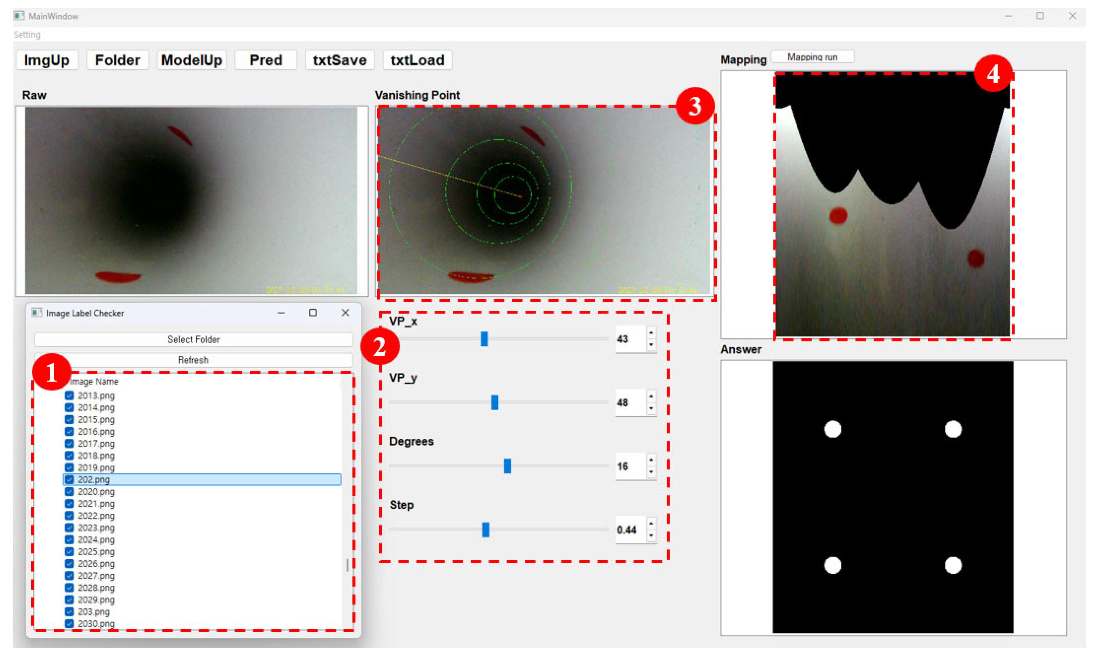
To annotate the collected inspection data with the corresponding back-projection parameters, a dedicated annotation toolkit was developed, as shown in Figure 4. The toolkit enables efficient and precise labeling of the key geometric features defined in Section 2.1, including the vanishing points and centerlines, without the need for additional sensing equipment. Instead, a reference marker of known geometry was placed within the pipeline to establish the ground truth for the spatial-scale calibration.

The annotation interface is structured as follows:

➀

A window displaying the current state of the inspection dataset.

➁

Scrollbars and text boxes for inputting numerical values of the parameters.

➂

A rendered image frame highlighting annotated features such as vanishing points.

➃

Unwrapped 2D projection of cylindrical pipe, aiding in the visual consistency of the annotation.

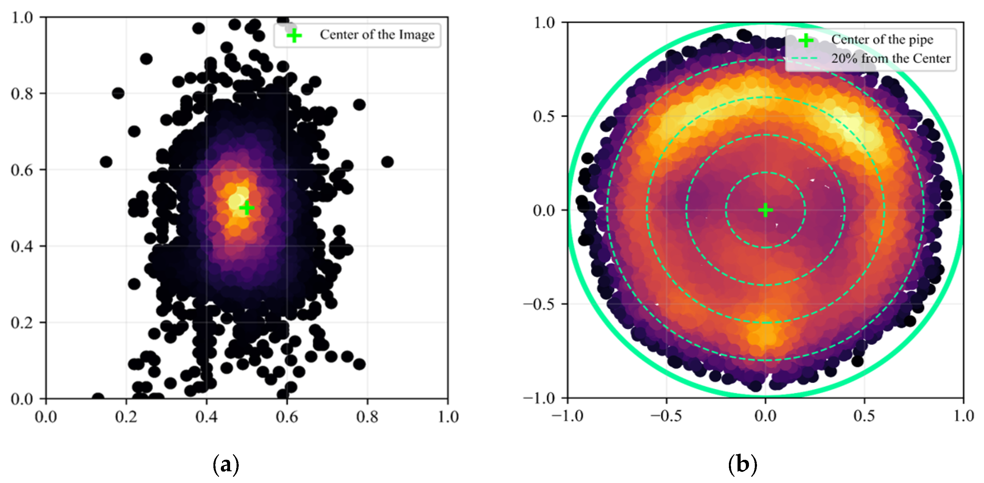
Using this toolkit, 9379 images were annotated, including 337 images obtained from previously conducted real-world in-service inspections and 9042 images generated under controlled experimental conditions. The spatial distribution of the key geometric features across the dataset is shown in Figure 5. As shown in Figure 5a, the vanishing point locations were primarily distributed within the central ±20% region of the image width. This distribution reflects the constrained rotation of the camera head, which is often restricted in operational settings to capture the full internal circumference of the pipe. As shown in Figure 5b, the camera position estimated by projecting the lens head location onto the image tends to cluster between 60% and 70% of the image height. This clustering is attributed to the relative positioning of the camera head within the pipelines of various diameters.

By incorporating heterogeneous imaging conditions, pipe materials, and defect structures, this dataset enables robust model generalization across different pipeline inspection scenarios. Moreover, the annotation strategy grounded in geometric references and visual features facilitates the accurate regression of back-projection parameters, which is crucial for reliable 3D reconstruction and defect quantification.

2.3. AI-Based Back-Projection Parameter Estimation Model

To estimate the back-projection parameters from monocular inspection images of water pipelines, a residual neural network (ResNet) originally proposed by He et al. [31] was employed in this study. ResNet is a deep convolutional neural network (CNN) architecture that introduces the concept of residual learning to alleviate the degradation problems encountered in deep networks. By leveraging identity mappings across shortcut connections, ResNet facilitates effective training of deep networks and has demonstrated superior performance in a variety of visual tasks. ResNet has been successfully utilized in heuristic-free feature extraction tasks such as road segmentation for autonomous driving [32], road marking recognition [33], and vanishing point detection [34,35]. In addition, it has shown promising results in infrastructure maintenance and defect detection systems [36,37,38], as well as in clinical diagnostic imaging applications where it is used to identify disease-associated risk factors [39,40,41,42].

The complexity and computational demands of ResNet architectures vary depending on the network depth.

Table 2. Number of parameters and FLOPs for various ResNet architectures.

Layer Name	ResNet-18	ResNet-34	ResNet-50	ResNet-101	ResNet-152
Parameters	11.4 M	21.5 M	23.9 M	42.8 M	58.5 M
FLOPs	1.8 × 109	3.6 × 109	3.8 × 109	7.6 × 109	11.3 × 109

summarizes the number of trainable parameters and floating-point operations (FLOPs) required for a single forward pass across different ResNet variants.

Among the variants known for minimal classification errors, namely ResNet-50, ResNet-101, and ResNet-152, the ResNet-101 model was selected, considering its balance between depth and computational efficiency [43]. Global average pooling (GAP) [44] was applied before the fully connected layer to preserve the spatial integrity of the extracted features. The final architecture of the ResNet-101 model, as illustrated in Figure 6, accepts a three-channel RGB image with a resolution of 224 × 224 as the input and generates a spatially encoded feature map of size 7 × 7 × 2048. This output is then aggregated into a 1 × 1 × 2048 vector using GAP and passed to a regression layer to estimate the four back-projection parameters.

3. Experiments and Results

3.1. Training Results for the Back-Projection Parameter Estimation Model

The proposed model was trained using the environment detailed in

Table 3. Training Environment Specifications.

Hardware	Specification	Software	Specification
CPU	Inter Core i7-13700	Python	3.11.7
GPU	NVIDIA GeForce RTX 3060 12 GB	Pytorch	2.1.2
Memory capacity	32 GB	Operation System	Windows 10
Optimizer	Learning Rate	Epoch	Decrease rate
Adam	1 × 10−3	400	0.8/50 Epoch

. To mitigate overfitting and promote generalization, the dataset was shuffled every 50 epochs, and the learning rate was reduced to 80% of its previous value. The training utilized a hybrid loss function, as defined in Equations (13)–(15), which combines the mean absolute error (MAE) and mean squared error (MSE). This approach allows the network to suppress large errors during early training via the MSE, whereas the MAE contributes to stable convergence during later stages.

$$MAE={\displaystyle \frac{\sum |y-\widehat{y}|}{n}}$$

(13)

$$MSE={\displaystyle \frac{\sum {\left(y-\widehat{y}\right)}^2}{n}}$$

(14)

$$Loss function=0.5MAE+MSE$$

(15)

where y denotes the predicted value, ŷ the ground truth, and n the number of samples.

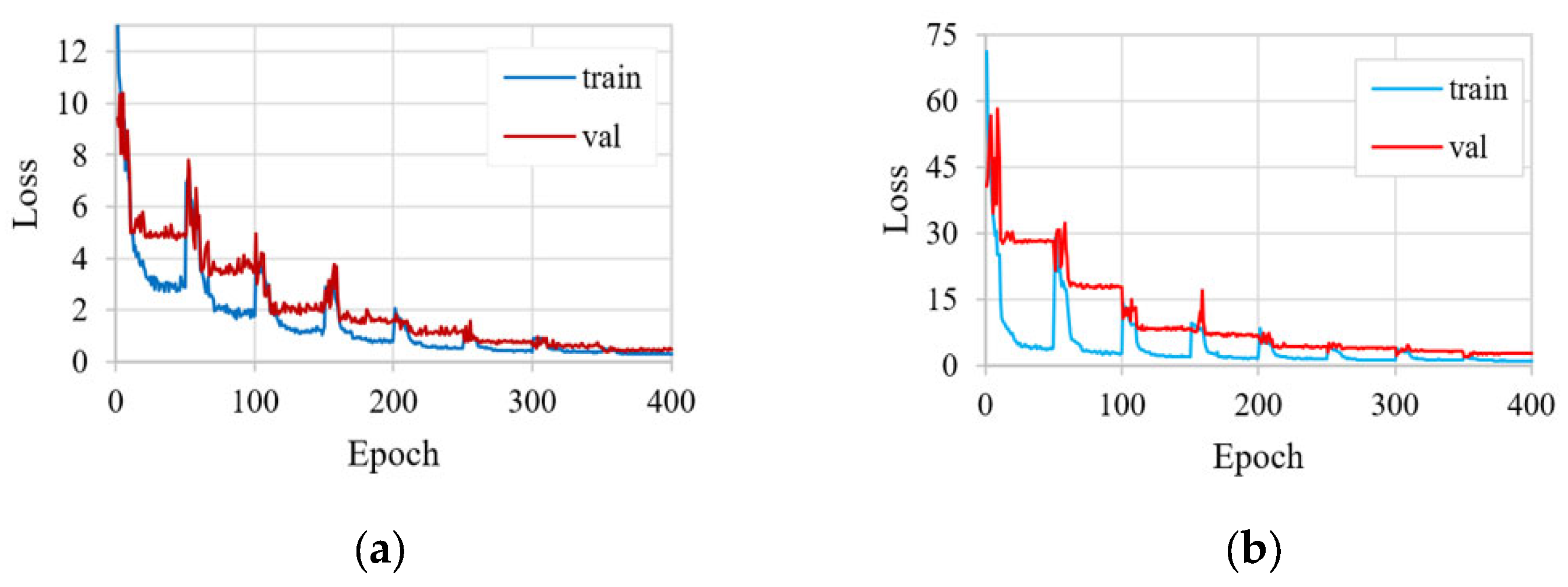
The training losses are shown in Figure 7. At the 398th epoch, the model yielded a rotation loss of 0.420 and a location loss of 2.665. The higher error associated with location estimation indicates that rotational features, particularly vanishing points, are more consistently identifiable than location-specific cues in monocular endoscopic images.

3.2. Accuracy Verification of Back-Projection Parameter Estimation

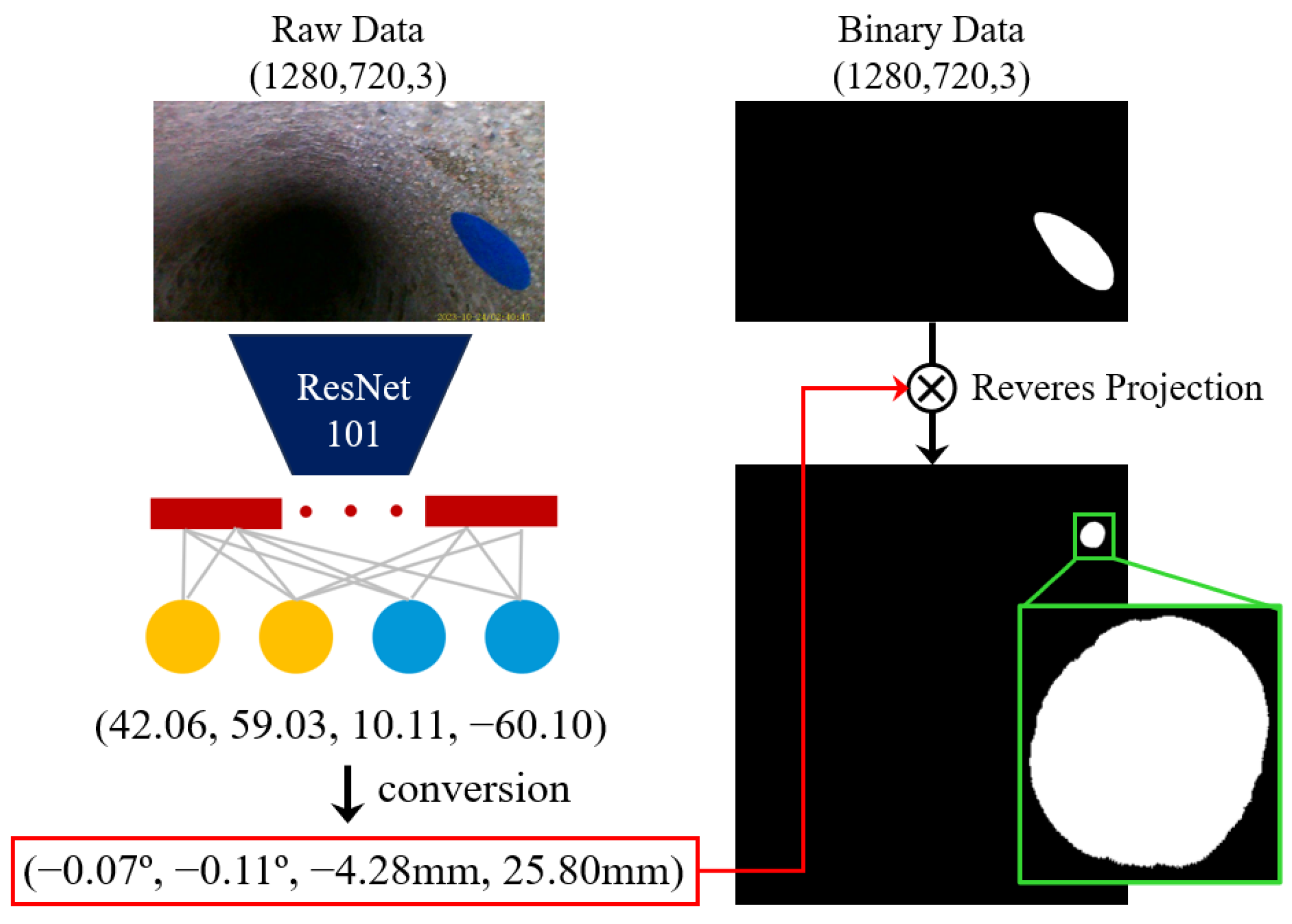
To validate the estimation accuracy, a binary reference marker image was generated using the predicted back-projection parameters from the original input containing the physical reference marker (Figure 8). The area of the marker in the reprojected image was measured and compared against a baseline approach using Hough circle detection.

Because the cylindrical projection preserves the spatial structure, the pixel area of the reference marker in the reprojected image reflects the actual physical area in mm². Error metrics, including absolute percentage error (APE) and mean absolute percentage error (MAPE), were calculated using Equations (16) and (17).

$$APE(\%)=100·\sum |{\displaystyle \frac{A-\widehat{A}}{\widehat{A}}}|$$

(16)

$$MAPE(\%)={\displaystyle \frac{100}{n}}·\sum |{\displaystyle \frac{A-\widehat{A}}{\widehat{A}}}|$$

(17)

where A is the area of the reprojected marker, Â is the true pixel area of a 19 mm reference circle, and n is the number of samples. In total, 308 validation images were used across different pipe types: cast iron pipe (CIP) 100, steel pipe (SP) 30, PVC 91, and paper pipe (PP) 87.

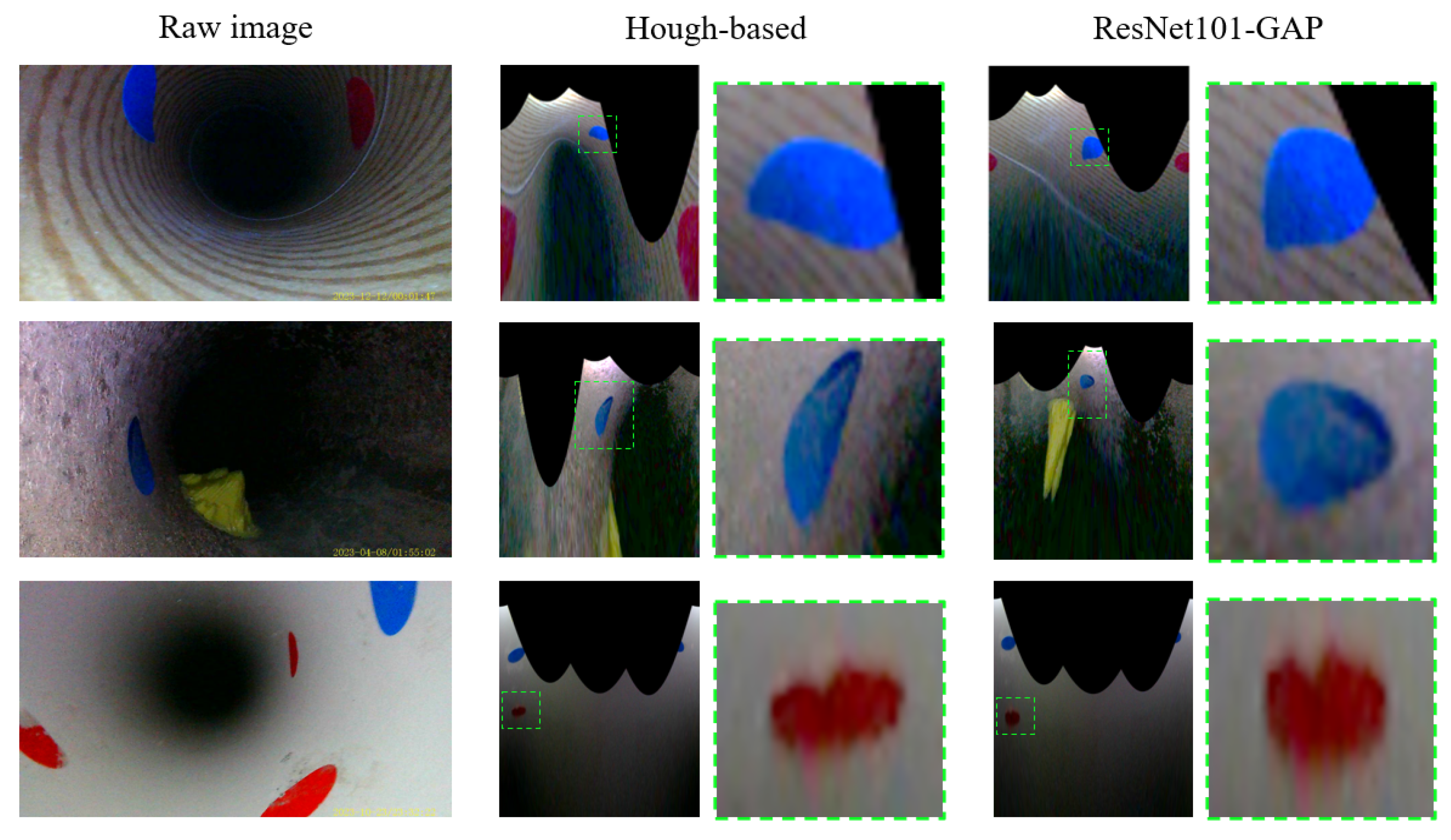
The results are summarized in

Table 4. Area accuracy comparison between methods.

Type	Diameter	Number of Data	Hough-Based				ResNet101-GAP
			MAPE	Top5	Bottom5	Miss Rate	MAPE	Top5	Bottom5
CIP	86 mm	100	181	3.2	1056.8	53/100	10.7	0.7	26.4
SP	34 mm	30	132.9	2.6	558.4	0/30	6.2	0.9	14.6
PVC	84 mm	91	26.6	6.1	50.4	12/91	7.0	0.1	28.5
PP	32 mm	87	97.8	1.0	854.2	8/87	6.7	0.4	23.9
Summary		308	109.6	3.2	630.0		7.7	0.5	23.4
Inference speed			2000 ms				8 ms

. The proposed ResNet101-GAP model achieved an average MAPE of 7.7%, significantly outperforming the Hough-based approach, which exhibited a high variance and an average MAPE of 109.6%. Moreover, the top five results from the ResNet-based model had an average error of only 0.5%, compared with 3.2% for the Hough method. In contrast, the bottom five samples revealed significant differences: the Hough method yielded a 630.0% error, whereas the ResNet101-GAP model maintained a 23.4% error. Notably, the Hough method failed to detect the marker in up to 53% of the PVC images, owing to specular reflection and noise.

In terms of inference speed, the ResNet model processes a frame in 8 ms, which is up to 250 times faster than the Hough-based method (2000 ms/frame), making it highly suitable for real-time applications.

The qualitative evaluations of the bottom-ranked APE samples are shown in Figure 9. In scenarios with poor lighting or occlusions, the Hough-based method failed to reliably detect the circular markers, resulting in significant errors. By contrast, the ResNet101-GAP model maintained stable predictions, demonstrating superior generalizability under various environmental constraints.

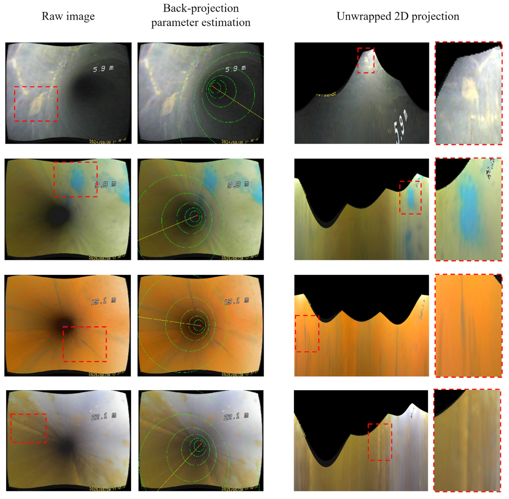
In practical inspections, noise introduced by camera motion—such as motion blur, highly colored defects, occlusions, turbulence effects, and variations in pipeline materials—is not as controlled or refined as the data obtained under experimental conditions. Therefore, we conducted a qualitative evaluation of the unwrapped 2D projection of cylindrical pipes transformed using deep-learning-based back-projection parameter estimation under various realistic noise conditions. First, as shown in Figure 10, qualitative evaluation of real inspection data where defects could be recognized demonstrates that perspective-aware unwrapped 2D projection is achievable regardless of variations in pipeline materials.

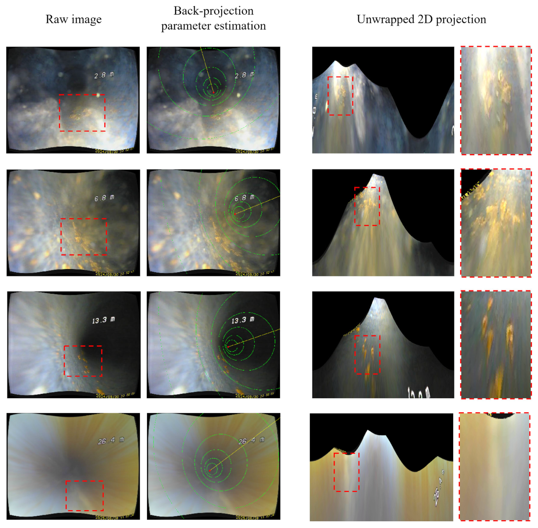
Furthermore, as illustrated in Figure 11, even under strong noise conditions caused by camera motion, such as motion blur, occlusions, and turbulence, the method can perform back-projection parameter estimation while accounting for cylindrical illumination conditions (darker at a distance, brighter when closer). However, although back-projection parameter estimation remains possible in such noisy environments, accurate defect recognition for quantitative evaluation can be highly challenging. Noise not only degrades the quality of the original endoscopic images but also propagates to the cylindrical projection, making defect boundaries unclear and leading to inaccuracies in quantitative assessment.

Since wired inspection cameras inevitably come into contact with the interior pipe surface, completely eliminating such noise is extremely challenging. To mitigate these potential limitations and obtain reliable inspection data, careful operational strategies are necessary. For instance, as illustrated in Figure 12, temporarily pausing to allow disturbed particles to settle sufficiently before identifying defects can help achieve more accurate measurements.

4. Conclusions

This paper proposes a deep-learning-based approach to estimate back-projection parameters from monocular endoscopic inspection images for the quantitative assessment of internal defects in cylindrical water pipelines. A mathematical framework was established to derive the relationships between image-space features such as vanishing points, pipeline centerlines, and extrinsic camera parameters, which serve as essential inputs for accurate 3D back-projection. To implement this framework, a ResNet-101 convolutional neural network augmented with global average pooling (GAP) was utilized to regress four key parameters: translation along the X and Y axes and rotation around the X and Y axes.

A hybrid dataset was constructed comprising both real-world in-service inspection images and experimentally generated data across a variety of pipe materials, diameters, and environmental conditions. An annotation toolkit was developed to manually label the back-projection parameters and geometric features using reference markers, enabling the generation of a well-structured dataset of 9379 labeled images. Experimental validation showed that the proposed AI model achieved significantly lower mean absolute percentage errors (MAPE: 7.7%) than conventional Hough-transform-based methods (MAPE: 109.6%). The model also demonstrated high robustness across different pipe types and imaging conditions, including reflective surfaces and varying camera positions. Notably, the proposed approach significantly improves the processing speed, achieving inference times of approximately 8 ms per frame, making it highly suitable for real-time applications.

Despite these promising results, this study has several limitations that warrant further investigation. First, the model was trained and validated on static single-frame data, which does not capture temporal dynamics or camera motion information present in video sequences. Second, the manual annotation of four back-projection parameters is labor-intensive and requires considerable effort. Third, although the model demonstrates generalizability under challenging conditions such as turbulence, biofilm coverage, and variations in pipeline materials, these factors hinder accurate quantitative defect measurement.

To address these limitations, future research should incorporate temporal modeling using recurrent or transformer-based architectures. Given that inspection cameras typically operate under restricted motion, incorporating temporal cues such as frame rate and inter-frame camera dynamics is expected to reduce errors compared with inferences based solely on single frames. In addition, although four back-projection parameters were manually annotated in this study, future work should explore weak or semi-supervised learning approaches that enable regression using partially annotated data combined with unannotated data. Expanding the dataset to include more severe environmental conditions and applying domain adaptation techniques could further enhance model robustness. During dataset expansion, careful operation of inspection equipment is essential to obtain refined data that support accurate quantitative defect assessment.

In summary, the proposed approach demonstrates a significant advancement in the automatic estimation of spatial parameters from monocular inspection images and lays the foundation for the future development of intelligent pipeline assessment systems capable of operating under diverse and dynamic field conditions.

References

1. Ministry of Environment Korea. Water Supply Statistics; Ministry of Environment Korea: Sejong, Republic of Korea, 2023. [Google Scholar]
2. Jun, H.J.; Park, J.K.; Bae, C.H. Factors affecting steel water-transmission pipe failure and pipe-failure mechanisms. J. Environ. Eng. 2020, 146, 04020034. [Google Scholar] [CrossRef]
3. Taiwo, R.; Shaban, I.A.; Zayed, T. Development of sustainable water infrastructure: A proper understanding of water pipe failure. J. Clean. Prod. 2023, 398, 136653. [Google Scholar] [CrossRef]
4. Mukunoki, T.; Kumano, N.; Otani, J.; Kuwano, R. Visualization of three dimensional failure in sand due to water inflow and soil drainage from defective underground pipe using X-ray CT. Soils Found. 2009, 49, 959–968. [Google Scholar] [CrossRef]
5. Cui, J.; Liu, F.; Chen, R.; Wang, S.; Pu, C.; Zhao, X. Effects of internal pressure on urban water supply pipeline leakage-induced soil subsidence mechanisms. Geofluids 2024, 2024, 9577375. [Google Scholar] [CrossRef]
6. Jacobsz, S.W. Responsive Pipe Networks; Water Research Commission Report; Water Research Commission: Pretoria, South Africa, 2019. [Google Scholar]
7. Zhao, R.; Li, L.; Chen, X.; Zhang, S. Mechanical response of pipeline leakage to existing tunnel structures: Insights from numerical modeling. Buildings 2025, 15, 1771. [Google Scholar] [CrossRef]
8. Rajani, B.; Kleiner, Y. Non-destructive inspection techniques to determine structural distress indicators in water mains. Eval. Control. Water Loss Urban Water Netw. 2004, 47, 21–25. [Google Scholar]
9. Mazumder, R.K.; Salman, A.M.; Li, Y.; Yu, X. Performance evaluation of water distribution systems and asset management. J. Infrastruct. Syst. 2018, 24, 03118001. [Google Scholar] [CrossRef]
10. Bado, M.F.; Casas, J.R. A review of recent distributed optical fiber sensors applications for civil engineering structural health monitoring. Sensors 2021, 21, 1818. [Google Scholar] [CrossRef]
11. Abegaz, R.; Wang, F.; Xu, J.; Pierce, T. Developing soil internal erosion indicator to quantify erosion around defective buried pipes under water exfiltration. Geotech. Test. J. 2025, 48, 623–641. [Google Scholar]
12. Jahnke, S.I. Pipeline Leak Detection Using in-situ Soil temperature and Strain Measurements. Ph.D. Thesis, University of Pretoria, Pretoria, South Africa, 2018. [Google Scholar]
13. Dave, M.; Juneja, A. Erosion of soil around damaged buried water pipes a critical review. Arab. J. Geosci. 2023, 16, 317. [Google Scholar] [CrossRef]
14. Kumar, S.S.; Abraham, D.M.; Jahanshahi, M.R.; Iseley, T.; Starr, J. Automated defect classification in sewer closed circuit television inspections using deep convolutional neural networks. Automat. Construct. 2018, 91, 273–283. [Google Scholar] [CrossRef]
15. Meijer, D.; Scholten, L.; Clemens, F.; Knobbe, A. A defect classification methodology for sewer image sets with convolutional neural networks. Automat. Construct. 2019, 104, 281–298. [Google Scholar] [CrossRef]
16. Dang, L.M.; Kyeong, S.; Li, Y.; Wang, H.; Nguyen, T.N.; Moon, H. Deep learning-based sewer defect classification for highly imbalanced dataset. Comput. Ind. Eng. 2021, 161, 107630. [Google Scholar] [CrossRef]
17. Moradi, S.; Zayed, T. Defect Detection and Classification in Sewer Pipeline Inspection Videos Using Deep Neural Networks. Ph.D. Thesis, Concordia University, Montreal, QC, Canada, 2020. [Google Scholar]
18. Shen, D.; Liu, X.; Shang, Y.; Tang, X. Deep learning-based automatic defect detection method for sewer pipelines. Sustainability 2023, 15, 9164. [Google Scholar] [CrossRef]
19. Sun, L.; Zhu, J.; Tan, J.; Li, X.; Li, R.; Deng, H.; Zhang, X.; Liu, B.; Zhu, X. Deep learning-assisted automated sewage pipe defect detection for urban water environment management. Sci. Total Environ. 2023, 882, 163562. [Google Scholar] [CrossRef] [PubMed]
20. Zhang, J.; Liu, X.; Zhang, X.; Xi, Z.; Wang, S. Automatic detection method of sewer pipe defects using deep learning techniques. Appl. Sci. 2023, 13, 4589. [Google Scholar] [CrossRef]
21. Li, Y.; Wang, H.; Dang, L.M.; Piran, M.J.; Moon, H. A robust instance segmentation framework for underground sewer defect detection. Measurement 2022, 190, 110727. [Google Scholar] [CrossRef]
22. Jung, J.T.; Reiterer, A. Improving sewer damage inspection: Development of a deep learning integration concept for a multi-sensor system. Sensors 2024, 24, 7786. [Google Scholar] [CrossRef]
23. Mostafa, K.; Hegazy, T. Review of image-based analysis and applications in construction. Automat. Construct. 2021, 122, 103516. [Google Scholar] [CrossRef]
24. Liu, J.C.; Tan, Y.; Wang, Z.Y.; Long, Y.Y. Experimental and numerical investigation on internal erosion induced by infiltration of defective buried pipe. Bull. Eng. Geol. Environ. 2025, 84, 38. [Google Scholar] [CrossRef]
25. Pridmore, T.P.; Cooper, D.; Taylor, N. Estimating camera orientation from vanishing point location during sewer surveys. Automat. Construct. 1997, 6, 393–401. [Google Scholar]
26. Kolesnik, M.; Baratoff, G. 3D interpretation of sewer circular structures. In Proceedings of the 2000 ICRA, IEEE International Conference on Robotics and Automation, Paris, France, 31 May–4 June 2020; IEEE: New York, NY, USA, 2020; Volume 4, pp. 3770–3775. [Google Scholar]
27. Kwon, G.O.; Kwon, H.G.; Choi, Y.H. Development of computer vision-based water pipe internal defect quantification technique. J. Korea Water Resour. Assoc. 2024, 57, 835–845. [Google Scholar]
28. Hengmeechai, J. Automated Analysis of Sewer Inspection Closed Circuit Television Videos Using Image Processing Techniques. Master’s Thesis, University of Waterloo, Waterloo, ON, Canada, 2013. [Google Scholar]
29. Brammer, K. Feasibility of Active Vision for Inspection of Continuous Concrete Pipes. Ph.D. Thesis, Sheffield Hallam University, Sheffield, UK, 2003. [Google Scholar]
30. Dawson-Howe, K.M.; Vernon, D. Simple pinhole camera calibration. Int. J. Imaging Syst. Technol. 1994, 5, 1–6. [Google Scholar] [CrossRef]
31. He, K.; Zhang, X.; Ren, S.; Sun, J. Deep residual learning for image recognition. In Proceedings of the IEEE Conference on Computer Vision and Pattern Recognition, Las Vegas, NV, USA, 26 June–1 July 2016; IEEE: New York, NY, USA, 2016; pp. 770–778. [Google Scholar]
32. Fan, R.; Wang, Y.; Qiao, L.; Yao, R.; Han, P.; Zhang, W.; Pitas, I.; Liu, M. PT-ResNet: Perspective transformation-based residual network for semantic road image segmentation. In Proceedings of the 2019 IEEE International Conference on Imaging Systems and Techniques (IST), Abu Dhabi, United Arab Emirates, 8–10 December 2019; IEEE: New York, NY, USA, 2019; pp. 1–5. [Google Scholar]
33. Hoang, T.M.; Nam, S.H.; Park, K.R. Enhanced detection and recognition of road markings based on adaptive region of interest and deep learning. IEEE Access 2019, 7, 109817–109832. [Google Scholar] [CrossRef]
34. Choi, H.S.; An, K.; Kang, M. Regression with residual neural network for vanishing point detection. Image Vision Comput. 2019, 91, 103797. [Google Scholar] [CrossRef]
35. Li, X.; Zhu, L.; Yu, Z.; Guo, B.; Wan, Y. Vanishing point detection and rail segmentation based on deep multi-task learning. IEEE Access 2020, 8, 163015–163025. [Google Scholar] [CrossRef]
36. Cheng, J.C.; Wang, M. Automated detection of sewer pipe defects in closed-circuit television images using deep learning techniques. Automat. Construct. 2018, 95, 155–171. [Google Scholar]
37. Halfawy, M.R.; Hengmeechai, J. Integrated vision-based system for automated defect detection in sewer closed circuit television inspection videos. J. Comput. Civil Eng. 2015, 29, 04014065. [Google Scholar] [CrossRef]
38. Kagami, S.; Taira, H.; Miyashita, N.; Torii, A.; Okutomi, M. 3D pipe network reconstruction based on structure from motion with incremental conic shape detection and cylindrical constraint. In Proceedings of the 2020 IEEE 29th International Symposium on Industrial Electronics (ISIE), Delft, The Netherlands, 17–19 June 2020; IEEE: New York, NY, USA, 2020; pp. 1345–1352. [Google Scholar]
39. Zheng, Z.; Zhang, H.; Li, X.; Liu, S.; Teng, Y. ResNet-based model for cancer detection. In Proceedings of the 2021 IEEE International Conference on Consumer Electronics and Computer Engineering (ICCECE), Guangzhou, China, 15–17 January 2021; IEEE: New York, NY, USA, 2021; pp. 325–328. [Google Scholar]
40. Praveen, S.P.; Srinivasu, P.N.; Shafi, J.; Wozniak, M.; Ijaz, M.F. ResNet-32 and FastAI for diagnoses of ductal carcinoma from 2D tissue slides. Sci. Rep. 2022, 12, 20804. [Google Scholar]
41. Mehnatkesh, H.; Jalali, S.M.J.; Khosravi, A.; Nahavandi, S. An intelligent driven deep residual learning framework for brain tumor classification using MRI images. Exp. Syst. Appl. 2023, 213, 119087. [Google Scholar] [CrossRef]
42. Gopi, A.; Sudha, L.R.; Thanakumar, J.S.I. Resnet for blood sample detection: A study on improving diagnostic accuracy. AG Salud 2025, 3, 193. [Google Scholar] [CrossRef]
43. Khan, A.; Sohail, A.; Zahoora, U.; Qureshi, A.S. A survey of the recent architectures of deep convolutional neural networks. Artif. Intell. Rev. 2020, 53, 5455–5516. [Google Scholar] [CrossRef]
44. Lin, M.; Chen, Q.; Yan, S. Network in network. arXiv 2013, arXiv:1312.4400. [Google Scholar]
Figure 1. Flowchart of AI-based endoscopic inspection image back-projection parameter estimation model development.
Mathematics 13 03291 g001
Figure 2. Image features arising from imaging a cylindrical surface.
Mathematics 13 03291 g002
Figure 3. Vanishing point variation with a single rotation.
Mathematics 13 03291 g003
Figure 4. Toolkit for annotating back−projection parameters from monocular endoscopic inspection images.
Mathematics 13 03291 g004
Figure 5. Distribution visualization of annotated dataset features. (a) Distribution of vanishing points across image width. (b) Vertical distribution of camera position estimates. Where brighter colors indicate higher data density, meaning that samples are more concentrated in those regions.
Mathematics 13 03291 g005
Figure 6. ResNet-101 architecture with GAP for back-projection parameter estimation.
Mathematics 13 03291 g006
Figure 7. Training Loss Curves: (a) Rotation Loss. (b) Location Loss.
Mathematics 13 03291 g007
Figure 8. Accuracy verification method using reprojected marker area. Where the red box represents the estimated camera pose (rotation and translation along the X- and Y-axes), and the green box shows an enlarged view of the marker in the unwrapped 2D projection.
Mathematics 13 03291 g008
Figure 9. Qualitative evaluation of high-APE samples across detection methods. Where the green box indicates a magnified view of the marker.
Mathematics 13 03291 g009
Figure 10. Qualitative evaluation of Back-Projection Parameter Estimation under relatively refined conditions. Where the red box in the raw image and the red box in the unwrapped 2D projection indicate the same corresponding region.
Mathematics 13 03291 g010
Figure 11. Qualitative evaluation of Back-Projection Parameter Estimation under severe noise conditions. Where the red box in the raw image and the red box in the unwrapped 2D projection indicate the same corresponding region.
Mathematics 13 03291 g011
Figure 12. Example of back-projection with recognizable defects for quantitative measurement. Where the red box in the raw image and the red box in the unwrapped 2D projection indicate the same corresponding region.
Mathematics 13 03291 g012