On Probabilistic Convergence Rates of Symmetric Stochastic Bernstein Polynomials

Abstract

This paper analyzes the exponential convergence properties of Symmetric Stochastic Bernstein Polynomials (SSBPs), a novel approximation framework that combines the deterministic precision of classical Bernstein polynomials (BPs) with the adaptive node flexibility of Stochastic Bernstein Polynomials (SBPs). Through innovative applications of order statistics concentration inequalities and modulus of smoothness analysis, we derive the first probabilistic convergence rates for SSBPs across all $L_p$ ($1\le p\le \infty$) norms and in pointwise approximation. Numerical experiments demonstrate dual advantages: (1) SSBPs achieve comparable $L_{\infty }$ errors to BPs in approximating fundamental stochastic functions (uniform distribution and normal density), while significantly outperforming SBPs; (2) empirical convergence curves validate exponential decay of approximation errors. These results position SSBPs as a principal solution for stochastic approximation problems requiring both mathematical rigor and computational adaptability.

1. Introduction

Modern engineering systems increasingly rely on function approximation from irregular measurements, for example, medical imaging reconstruction [1], robotic sensor networks [2], and shape design problems [3], to name a few. During various approximation methods, classical Bernstein polynomials exhibit excellent properties and have broad applications [4,5,6,7]. For a function $f\in C[0,1]$, the degree n Bernstein polynomial $B_{n}f$ is constructed as follows:

$$B_{n}f(t)=\sum _{k=0}^{n}f\left({\displaystyle \frac{k}{n}}\right)B_k^n(t),t\in [0,1],$$

where $B_k^n(t)=\left({\displaystyle \genfrac{}{}{0pt}{}{n}{k}}\right)t^k{(1-t)}^{n-k}$, and $\left({\displaystyle \genfrac{}{}{0pt}{}{n}{k}}\right)$ represents the binomial coefficient. This polynomial approximates the function f in the Banach space $C[0,1]$, and the approximation error is bounded by the inequality (see, e.g., [8]):

$$\parallel B_n{f(t)-f(t)\parallel }_{C[0,1]}\le {\omega }_2\left(f,{\displaystyle \frac{1}{\sqrt{n}}}\right),f\in C[0,1],$$

(1)

where the second-order modulus of smoothness ${\omega }_2(f,h)$ is defined as:

$${\omega }_2(f,h):=\underset{\begin{array}{c}t\pm \tau \in [a,b]\\ |\tau |\le h\end{array}}{sup}|f(t+\tau )+f(t-\tau )-2f(t)|.$$

(2)

However, as Wu et al. [9] pointed out, their performance may be limited when handling scattered or noisy data. They can also face challenges in accurately approximating complex functions in high-dimensional spaces. In many real-world problems, data at equally spaced points may not be available, and even when it appears evenly distributed, it may suffer from random errors caused by signal delays or measurement inaccuracies.

Let X be the random variable uniformly distributed on $[0,1]$. Let ${\{X_{n,k}\}}_{k=0}^n$ be $(n+1)$ independent copies of X, which we list in ascending order (Here, we have ignored the event: some of the random variables take the same value, which has probability zero).

$$X_{n,0}^{*}<X_{n,1}^{*}<\dots <X_{n,n}^{*},$$

to obtain ordered statistics [10]. For brevity of notation, we suppress the asterisks in the displayed inequalities above, and stick with the notations ${\{X_{n,k}\}}_{k=0}^n$ for order statistics.

To mitigate uncertainties brought on by unreliable sampling sites, Wu et al. [9] introduced a class of SBP:

$$B_n^{X}f(t):=\sum _{k=0}^{n}f(X_{n,k})B_k^n(t),$$

(3)

and proved the following result: Let $ϵ>0$ and suppose that ${\displaystyle \omega \left(f,\frac{1}{\sqrt{n}}\right)<\frac{ϵ}{4.2}.}$ Then,

$$\mathbb{P}\left\{\parallel B_n^X{f(t)-f(t)\parallel }_{\infty }>ϵ\right\}\le {\displaystyle \frac{15}{64}}·{\displaystyle \frac{n{\omega }^6\left(f,\frac{1}{\sqrt{n}}\right)}{{ϵ}^6}},$$

in which $\omega \left(f,·\right)$ denotes the modulus of continuity of f defined by

$$\omega (f,h):=\underset{\begin{array}{c}0\le x,y\le 1\\ |x-y|\le h\end{array}}{sup}\left|f(x)-f(y)\right|,0\le h\le 1.$$

Sun et al. [11,12,13] analyzed the polynomial error of the classical SBP method. Adell and Cárdenas-Morales [14,15,16] have recently introduced a type of SBPs which enhance probabilistic error estimates for smooth functions. On that basis, Gao et al. [17,18] constructed a series of stochastic quasi-interpolations for scattered data problems, which showed efficiency in computation and high accuracy in approximation. Gal et al. [19] examined efficient approximation methods for random functions using stochastic Bernstein polynomials within capacity spaces. Bouzebda [20] combined k-nearest neighbors with single index modeling to handle high-dimensional functional mixing data through dimension reduction, effectively mitigating the curse of dimensionality. These estimates are similar to those established in the learning theory paradigm advocated by Cucker and Smale [21] and Cucker and Zhou [22].

Moreover, Wu et al. [12] analyzed the exponential convergence of SBP, which is crucial for stochastic problems in practice, such as probability density estimation, numerical solutions to stochastic differential equations, and denoising problems. Taking these factors into account, Sun [12] conducted an analysis of the exponential convergence of the classical SBP method. In order to analyze the overall error of SBPs, Sun [12] introduced the concept of “$L_p$-probabilistic convergence” for SBP: For $1\le p\le \infty$ and $f\in C[0,1]$, we define

$${\parallel f\parallel }_p:=\left\{\begin{array}{cc}{\left({\int }_0^1{|f(t)|}^{p}dt\right)}^{1/p},\hfill & \mathrm{if}1\le p<\infty ,\hfill \\ \underset{t\in [0,1]}{max}|f(t)|,\hfill & \mathrm{if}p=\infty .\hfill \end{array}\right.$$

On that basis, they gave the power and exponential convergence rates using the modulus of continuity and established Gaussian tail bounds $1\le p\le 2$, and the case $p=\infty$. The pointwise exponential error estimate is also given.

In order to improve the approximation power of SBPs and let it possess the same approximation power of the classical Bernstein polynomials given by Equation (1), Gao et al. [23] introduced a family of symmetric stochastic Bernstein polynomials (SSBPs) which is called optimal in the sense that it possess the same order of error estimates as classical Bernstein polinomials. The SSBPs is defined as

$$B_n^{T}f(t):={\displaystyle \frac{1}{2}}\sum _{k=0}^n\left[f(X_{n,k})+f(Y_{n,k})\right]B_k^n(t),$$

(4)

in which $Y_{n,k}={\displaystyle \frac{2k}{n}}-X_{n,k}$. SSBPs are stochastic variants of classical Bernstein polynomials. Among other flexible features, SSBPs allow the underlying sampling operation to take place at scattered sites, which is a more practical way of collecting data for many real world problems. Ref. [23] established the order of convergence in probability in terms of modulus of smoothness, which epitomizes an optimal pointwise error estimate for the classical Bernstein polynomial approximation. Given $ϵ>0$ and assume that ${\omega }_{\phi }^2(f,{\displaystyle \frac{1}{\sqrt{n}}})<{\displaystyle \frac{ϵ}{33}}$. Then, for any $0\le t\le 1$, the following probabilistic estimate holds true:

$$\begin{array}{c}\hfill \mathbb{P}\left\{\left|B_n^{T}f(t)-f(t)\right|>ϵ\right\}\le 152{\displaystyle \frac{max\left(59{\left[{\omega }_{\phi }^2\left(f,\frac{1}{\sqrt{n}}\right)\right]}^2,100{\left[{\omega }^2\left(f,\frac{1}{n}\right)\right]}^2\right)}{{ϵ}^2}},\end{array}$$

(5)

where the second-order Ditzian–Totik $\phi$-modulus of smoothness is defined by

$${\omega }_{\phi }^2(f,h)=\underset{\begin{array}{c}t\pm \phi (t)\tau \in [0,1]\\ |\tau |\le h\end{array}}{sup}|f(t+\phi (t)\tau )+f(t-\phi (t)\tau )-2f(t)|,h\ge 0,$$

which characterizes the approximation order of $B_{n}f$ to f in the Banach space $C[0,1]$.

Motivated by the method in [12], this paper studies the exponential convergence of SSBP. By employing concentration inequalities for order statistics and properties of the modulus of smoothness, we establish probabilistic convergence rates for SSBPs in both the $L_p$ norm, for $0<p\le \infty$, and pointwise. Numerical experiments approximating two standard functions demonstrate that SSBPs achieve approximation errors comparable to those of classical Bernstein polynomials while outperforming SBPs. SSBPs present a promising tool for function approximation in stochastic settings, particularly when dealing with scattered and noisy data, and open new avenues for research in stochastic approximation theory and numerical solutions of stochastic partial differential equations.

The paper is structured as follows: Section 2 covers the necessary preliminaries. Section 3 presents error estimates for the exponential convergence in the $L_p$ norm, while Section 4 addresses pointwise exponential convergence estimates. In Section 5, numerical examples are provided to validate the theoretical findings. Finally, Section 6 concludes the paper with a summary of the key results and potential directions for future research.

2. Preliminaries

2.1. Concentration Inequalities for Order Statistics

For a given $n\in \mathbb{N}$, let

$$0\le X_{n,0}<X_{n,1}<\cdots <X_{n,n}\le 1,$$

(6)

be the order statistics of $(n+1)$ independent copies of the random variable X uniformly distributed in $(0,1)$. The following is a standard result in order statistics (e.g., [10,24]).

Theorem 1.

If X is a random variable that has density function $f(x)$ and distribution function $F(x)$, and if

$$X^{(1)}<X^{(2)}<\cdots <X^{(n)}$$

are the order statistics of the n sample values of X, then the density function $f_{X^{(j)}}$ of $X^{(j)}$ is given by

$$f_{X^{(j)}}(x)={\displaystyle \frac{n!}{(j-1)!(n-j)!}}{[F(x)]}^{(j-1)}{[1-F(x)]}^{(n-j)}f(x).$$

Proposition 1.

The random variables $X_{n,k}$ (as described in (6)) have, respectively, density functions: $p_{n,k}(x):=(n+1)·B_k^n(x),k=0,1,\dots ,n$. That is, $X_{n,k}$ obeys the law $B(k+1,n-k+1)$, the beta distribution with parameters $k+1$ and $n-k+1.$

Order statistics are intrinsically dependent random variables, and must be studied as such. Direct calculation gives

$$\begin{array}{cc}\hfill & \mathbb{E}(X_{n,k})={\displaystyle \frac{k+1}{n+2}},\mathrm{and}\hfill \\ \hfill & \mathrm{Var}(X_{n,k})={\displaystyle \frac{(k+1)(n-k+1)}{{(n+2)}^2(n+3)}}.\hfill \end{array}$$

(7)

For $0\le j<k\le n$, the covariance $\mathrm{Cov}(X_{n,j},X_{n,k})$ of the two random variables $X_{n,j},X_{n,k}$ is

$$\begin{array}{cc}\hfill \mathrm{Cov}(X_{n,j},X_{n,k})& ={\displaystyle \frac{(j+1)(n-k+1)}{{(n+2)}^2(n+3)}}.\hfill \end{array}$$

(8)

The last equation can be found in [10]. Recall that $Y_{n,k}={\displaystyle \frac{2k}{n}}-X_{n,k}$. It then follows that

$$\begin{array}{cc}\hfill & \mathbb{E}(Y_{n,k})={\displaystyle \frac{2k}{n}}-{\displaystyle \frac{k+1}{n+2}},\mathrm{Cov}(Y_{n,j},Y_{n,k})=\mathrm{Cov}(X_{n,j},X_{n,k}).\hfill \end{array}$$

2.2. Extension and Modulus of Continuity

It is noted that, the construct of an SSBP (4) requires that a target function be defined on $[-1,2]$. If a target function is already defined on $[-1,2]$, then nothing needs to be done. If a target function f is only defined on $[0,1]$, then we extend it to be a continuous function on $[-1,2]$ in such a way that the graph of f on the interval $[-1,0]([1,2])$ is symmetric to that on the interval $[0,1]$ with respect to the point $(0,f(0))((1,f(1))$. Precisely, we define the extension $f_E$ as follows:

$$f_E(t)=\left\{\begin{array}{ccc}\hfill & 2f(0)-f(-t),\hfill & \hfill -1\le t<0,\\ \hfill & f(t),\hfill & \hfill 0\le t\le 1,\\ \hfill & 2f(1)-f(2-t),\hfill & \hfill 1<t\le 2.\end{array}\right.$$

(9)

In [23], ${\omega }_2(f_E,h)$ is bounded from above by an (absolute) constant multiple of ${\omega }_2(f,h)$ in the following lemma.

Lemma 1.

Let $f\in C[0,1]$ and $f_E$ be the extension of f as defined in Equation (9), $0\le \tau \le h\le 1$. Then a central secnd-order finite difference of $f_E$ on $[-1,2]$: ${\Delta }_{\tau }^2{f}_E(t)=f_E(t+\tau )+f_E(t-\tau )-2f_E\left(t\right)$ is bounded above by that of f on $[0,1]$. Moreover, the following inequality holds true:

$$\begin{array}{c}\hfill {\omega }_2(f_E,h)\le 5{\omega }_2(f,h).\end{array}$$

(10)

3. Exponential Decay Rate of the ${\mathit{L}}_{\mathit{p}}$-Probabilistic Convergence

For consistency with contemporary literature, we adopt the functional norm definition initially introduced by Sun [12]. For $1\le p\le \infty$ and $f\in C[0,1]$, Sun [12] defined

$${\parallel f\parallel }_p:=\left\{\begin{array}{cc}{\left({\int }_0^1{|f(t)|}^{p}dt\right)}^{1/p},\hfill & \mathrm{if}1\le p<\infty ,\hfill \\ \underset{t\in [0,1]}{max}|f(t)|,\hfill & \mathrm{if}p=\infty .\hfill \end{array}\right.$$

3.1. $L_{\infty }$-Probabilistic Convergence

Lemma 2

([12]). If $X\sim Beta(\alpha ,\beta )$, then

$$\begin{array}{c}\hfill \mathbb{P}\{|X-\mathbb{E}(X)|>r\}\le 2exp\left[-2(\alpha +\beta +1)r^2\right],r>0.\end{array}$$

(11)

Lemma 3

([4]). If $f\in C[a,b]$ and $0\le \lambda ,h<\infty$, then

$$\begin{array}{cc}\hfill {\omega }^2(f,\lambda h)& \le {(1+\lambda )}^2{\omega }^2(f,h).\hfill \end{array}$$

(12)

In what follows, we will denote for each $n\in \mathbb{N}$ and $t\in [0,1]$,

$$\begin{array}{c}\hfill Z_n(t):=\sum _{k=0}^n{p}_{n,k}(t){\left[X_{n,k}-\mathbb{E}\left(X_{n,k}\right)\right]}^2.\end{array}$$

(13)

Our primary objective in this study is to establish rigorous upper bounds for the probability quantities:

$$\mathbb{P}\{\parallel B_n^{T}f-f{\parallel }_p>ϵ\},1\le p\le \infty ,$$

where $ϵ>0$ is a fixed error tolerance and $n\in \mathbb{N}$ represents the polynomial degree. To derive these estimates, we first require the following foundational lemma:

Lemma 4.

Let $ϵ>0$ and $f\in C[0,1]$ be given. Suppose that ${\omega }_2\left(f,{\displaystyle \frac{1}{\sqrt{n}}}\right)<{\displaystyle \frac{ϵ}{12+20/n}}$. Then the following inequality holds true:

$$\mathbb{P}\left\{{∥B_n^{T}f-f∥}_p>ϵ\right\}\le \mathbb{P}\left\{{∥Z_n∥}_p>{\displaystyle \frac{ϵ}{20n{\omega }_2\left(f,\frac{1}{\sqrt{n}}\right)}}\right\},1\le p\le \infty .$$

Proof. 

For a fixed $1\le p\le \infty$, we first use the $L_p$-space triangle inequality to write

$${∥B_n^{T}f-f∥}_p\le {∥B_{n}f-B_n^{T}f∥}_p+{∥B_{n}f-f∥}_p.$$

The second term can be estimated deterministically based on Equation (1):

$${∥B_{n}f-f∥}_p\le {∥B_{n}f-f∥}_{\infty }\le {\omega }_2\left(f,{\displaystyle \frac{1}{\sqrt{n}}}\right).$$

For the first term ${∥B_n^{T}f-B_{n}f∥}_p$, based on Equation (4) and the definition of $L_P$ norm, we have

$$\begin{array}{cc}\hfill \parallel B_n^{T}f-B_n{f\parallel }_p& \le {\left({\int }_0^1{\left|\sum _{k=0}^n{\displaystyle \frac{1}{2}}\left|f(X_{n,k})+f_E(Y_{n,k})-2f({\displaystyle \frac{k}{n}})\right|p_{n,k}(t)\right|}^{p}dt\right)}^{1/p}\hfill \\ & \le {\left({\int }_0^1{\left|\sum _{k=0}^n{\displaystyle \frac{1}{2}}{\omega }_2(f_E,\left|X_{n,k}-{\displaystyle \frac{k}{n}}\right|)p_{n,k}(t)\right|}^{p}dt\right)}^{1/p}\hfill \\ & \le {\left({\int }_0^1{\left|\sum _{k=0}^n{\displaystyle \frac{1}{2}}{\omega }_2(f_E,{\displaystyle \frac{1}{\sqrt{n}}}){(1+{\displaystyle \frac{\left|X_{n,k}-\frac{k}{n}\right|}{1/\sqrt{n}}})}^2{p}_{n,k}(t)\right|}^{p}dt\right)}^{1/p}\hfill \end{array}$$

where the last two inequalities are based on the definition of ${\omega }_2$ norm (Equation (2)). Then taking ${\omega }_2$ out, according to the Minkowski inequality and Lemma 1, we have:

$$\begin{array}{cc}& \parallel B_n^{T}f-B_n{f\parallel }_p\hfill \\ & \le {\omega }_2(f_E,{\displaystyle \frac{1}{\sqrt{n}}}){\left({\int }_0^1{\left|\sum _{k=0}^n(1^2+n{\left|X_{n,k}-{\displaystyle \frac{k}{n}}\right|}^2)p_{n,k}(t)\right|}^{p}dt\right)}^{1/p}\hfill \\ & \le {\omega }_2(f_E,{\displaystyle \frac{1}{\sqrt{n}}})+n{\omega }_2(f_E,{\displaystyle \frac{1}{\sqrt{n}}}){\left[{\int }_0^1{\left|\sum _{k=0}^n{\left(X_{n,k}-{\displaystyle \frac{k}{n}}\right)}^2{p}_{n,k}(t)\right|}^{p}dt\right]}^{1/p}\hfill \\ & \le 5{\omega }_2(f,{\displaystyle \frac{1}{\sqrt{n}}})+5n{\omega }_2(f,{\displaystyle \frac{1}{\sqrt{n}}}){\left[{\int }_0^1{\left|\sum _{k=0}^n{\left(X_{n,k}-{\displaystyle \frac{k}{n}}\right)}^2{p}_{n,k}(t)\right|}^{p}dt\right]}^{1/p}\hfill \\ & \le 5{\omega }_2(f,{\displaystyle \frac{1}{\sqrt{n}}})+5n{\omega }_2(f,{\displaystyle \frac{1}{\sqrt{n}}}){\left({\int }_0^1{\left|\sum _{k=0}^{n}2\left({\left[X_{n,k}-\mathbb{E}\left(X_{n,k}\right)\right]}^2+{\left[{\displaystyle \frac{k}{n}}-\mathbb{E}\left(X_{n,k}\right)\right]}^2\right)p_{n,k}(t)\right|}^{p}dt\right)}^{1/p}\hfill \\ & \le 5{\omega }_2(f,{\displaystyle \frac{1}{\sqrt{n}}})+5n{\omega }_2(f,{\displaystyle \frac{1}{\sqrt{n}}}){\left({\int }_0^1{\left|\sum _{k=0}^{n}2\left({\left[X_{n,k}-\mathbb{E}\left(X_{n,k}\right)\right]}^2+{\left({\displaystyle \frac{1}{n+1}}\right)}^2\right)p_{n,k}(t)\right|}^{p}dt\right)}^{1/p}\hfill \\ & \le \left(5+{\displaystyle \frac{10}{n}}\right){\omega }_2(f,{\displaystyle \frac{1}{\sqrt{n}}})+10n{\omega }_2(f,{\displaystyle \frac{1}{\sqrt{n}}}){∥Z_n∥}_p.\hfill \end{array}$$

Using the assumption that ${\omega }_2\left(f,{\displaystyle \frac{1}{\sqrt{n}}}\right)<{\displaystyle \frac{ϵ}{12+20/n}}$, we have

$$\left(6+{\displaystyle \frac{10}{n}}\right){\omega }_2(f,{\displaystyle \frac{1}{\sqrt{n}}})<{\displaystyle \frac{ϵ}{2}}.$$

Thus, in order for ${∥B_n^{T}f-f∥}_p>ϵ$ to hold true, it is necessary that

$${∥Z_n∥}_p>{\displaystyle \frac{ϵ}{20n{\omega }_2\left(f,\frac{1}{\sqrt{n}}\right)}},$$

which is the desired result. □

We are now in a position to present the first primary result of this work.

Theorem 2.

Let $ϵ>0$ and $f\in C[0,1]$ be given. Suppose that ${\omega }_2\left(f,{\displaystyle \frac{1}{\sqrt{n}}}\right)<{\displaystyle \frac{ϵ}{12+20/n}}$, then the following inequality holds true:

$$\begin{array}{cc}& \mathbb{P}\left\{{∥B_n^{T}f-f∥}_{\infty }>ϵ\right\}\hfill \\ & \le 2(n+1)exp\left(-{\displaystyle \frac{n+3}{10n}}{\displaystyle \frac{ϵ}{{\omega }_2\left(f,\frac{1}{\sqrt{n}}\right)}}\right)\hfill \end{array}$$

Proof. 

Let $ϵ>0$ and $f\in C([0,1])$ be given. Making use of Lemma 4 (for the case $p=\infty )$, we have

$$\begin{array}{cc}& \mathbb{P}\left\{{∥B_n^{T}f-f∥}_{\infty }>ϵ\right\}\hfill \\ \hfill \le & \mathbb{P}\left\{{∥Z_n∥}_{\infty }>{\displaystyle \frac{ϵ}{20n{\omega }_2\left(f,\frac{1}{\sqrt{n}}\right)}}\right\}\hfill \\ \hfill \le & \mathbb{P}\left\{\underset{0\le k\le n}{max}{\left|X_{n,k}-\mathbb{E}\left(X_{n,k}\right)\right|}^2>{\displaystyle \frac{ϵ}{20n{\omega }_2\left(f,\frac{1}{\sqrt{n}}\right)}}\right\}\hfill \\ \hfill \le & \sum _{k=0}^n\mathbb{P}\left\{{\left|X_{n,k}-\mathbb{E}\left(X_{n,k}\right)\right|}^2>{\displaystyle \frac{ϵ}{20n{\omega }_2\left(f,\frac{1}{\sqrt{n}}\right)}}\right\}\hfill \\ \hfill \le & 2(n+1)exp\left(-{\displaystyle \frac{n+3}{10n}}{\displaystyle \frac{ϵ}{{\omega }_2\left(f,\frac{1}{\sqrt{n}}\right)}}\right).\hfill \end{array}$$

This completes the proof. □

3.2. $L_p$-Probabilistic Convergence

For the case where $0<p<\infty$, the result exhibits stronger properties. To establish the main theorem, we require the following preparatory lemmas:

Lemma 5

([12]). Let $0<p<\infty$. Then

$$\mathbb{E}\left({\left|X_{n,k}-\mathbb{E}\left(X_{n,k}\right)\right|}^p\right)\le {\displaystyle \frac{p\mathsf{\Gamma }\left(\frac{p}{2}\right)}{2^{p/2}{(n+3)}^{p/2}}},k=0,1,\dots ,n.$$

Lemma 6.

For each $1\le p<\infty$, we have

$$\mathbb{E}{∥Z_n∥}_p^p\le {\displaystyle \frac{2p\mathsf{\Gamma }\left(p\right)}{2^p{(n+3)}^p}}.$$

Proof. 

We begin by noting that for each $k=0,1,\dots ,n$,

$${\int }_0^1{p}_{n,k}(t)dt={\displaystyle \frac{1}{n+1}}.$$

By applying Fubini’s theorem to interchange the order of integration between the Lebesgue integral over $t\in [0,1]$ and the expectation operator E, and leveraging the convexity of the function $f(x)=x^p$, we derive the following:

$$\begin{array}{cc}\hfill \mathbb{E}{∥Z_n∥}_p^p& ={\int }_0^1\mathbb{E}{\left(\sum _{k=0}^n{p}_{n,k}(t){\left|X_{n,k}-\mathbb{E}\left(X_{n,k}\right)\right|}^2\right)}^{p}dt\hfill \\ & \le {\int }_0^1\sum _{k=0}^n{p}_{n,k}(t)\mathbb{E}{\left|X_{n,k}-\mathbb{E}\left(X_{n,k}\right)\right|}^{2p}dt\hfill \\ & ={\displaystyle \frac{1}{n+1}}\sum _{k=0}^n\mathbb{E}{\left|X_{n,k}-\mathbb{E}\left(X_{n,k}\right)\right|}^{2p}\hfill \end{array}$$

We then apply Lemma 5 to get the desired result. □

Building upon the preceding lemmas, we now present the second principal result of this paper.

Theorem 3.

Let $ϵ>0$ and $1\le p<\infty$ be given. Suppose that $f\in C[0,1]$ satisfies

$${\omega }_2\left(f,{\displaystyle \frac{1}{\sqrt{n}}}\right)<{\displaystyle \frac{ϵ}{12+20/n}}.$$

Then, the following inequality holds true:

$$\mathbb{P}\left\{{∥B_n^T(f)-f∥}_p>ϵ\right\}\le {10}^p{n}^p\mathsf{\Gamma }\left(p\right){\displaystyle \frac{{\omega }_2^p\left(f,\frac{1}{\sqrt{n}}\right)}{{ϵ}^p}}.$$

Proof. 

For each $ϵ>0,p$ in the range $1\le p<\infty$, and $f\in C[0,1]$, we first recall the notation $Z_n$ defined in Equation (13) and then use Lemma 6 to write

$$\begin{array}{cc}& \mathbb{P}\left\{{∥B_n^{T}f-f∥}_p>ϵ\right\}\hfill \\ \hfill \le & \mathbb{P}\left\{{∥Z_n∥}_p>{\displaystyle \frac{ϵ}{20n{\omega }_2\left(f,\frac{1}{\sqrt{n}}\right)}}\right\}\hfill \\ \hfill =& \mathbb{P}\left\{{∥Z_n∥}_p^p>{\displaystyle \frac{{ϵ}^p}{{20}^p{n}^p{\omega }_2^p\left(f,\frac{1}{\sqrt{n}}\right)}}\right\}\hfill \\ \hfill \le & {20}^p{n}^p{\omega }_2^p\left(f,{\displaystyle \frac{1}{\sqrt{n}}}\right){\displaystyle \frac{\mathbb{E}{∥Z_n∥}_p^p}{{ϵ}^p}}\hfill \\ \hfill \le & {10}^p{n}^p\mathsf{\Gamma }\left(p\right){\displaystyle \frac{{\omega }_2^p\left(f,\frac{1}{\sqrt{n}}\right)}{{ϵ}^p}}\hfill \end{array}$$

where we have used the Markov inequality and Lemma 6.

This completes the proof. □

4. Exponential Decay of Pointwise Convergence in Probability

Sun and Wu [9] studied pointwise convergence in probability of the stochastic Bernstein polynomials defined in Equation (3) and proved the following result:

$$\mathbb{P}\left\{\left|B_n^{X}f(t)-f(t)\right|>ϵ\right\}\le 40{\displaystyle \frac{{\omega }^2\left(f,\frac{1}{\sqrt{n}}\right)}{{ϵ}^2}},\forall t\in [0,1].$$

In this section, we will prove the following theorem which is the third principal result of the paper.

Theorem 4.

Let $ϵ>0,f\in C[0,1]$, and $t\in [0,1]$ be given. Suppose that

$${\omega }_2\left(f,{\displaystyle \frac{1}{\sqrt{n}}}\right)<{\displaystyle \frac{ϵ}{12+20/n}}.$$

Then we have the following inequality

$$\mathbb{P}\left\{\left|B_n^{T}f(t)-f(t)\right|>ϵ\right\}\le 2exp\left[-{\displaystyle \frac{ϵ}{20{\omega }_2\left(f,\frac{1}{\sqrt{n}}\right)}}\right].$$

We need the following Lemmas to prove Theorem 4.

Lemma 7

([12]).

$$\mathbb{E}\left[exp\left(n\sum _{k=0}^n{p}_{n,k}(t){\left|X_{n,k}-\mathbb{E}\left(X_{n,k}\right)\right|}^2\right)\right]\le 2.$$

Lemma 8.

Let $ϵ>0$ and $f\in C[0,1]$ be given. Suppose that

$${\omega }_2\left(f,{\displaystyle \frac{1}{\sqrt{n}}}\right)<{\displaystyle \frac{ϵ}{12+20/n}}.$$

Then for each fixed $t\in [0,1]$, the following inequality holds true.

$$\mathbb{P}\left\{\left|B_n^{T}f(t)-f(t)\right|>ϵ\right\}\le \mathbb{P}\left\{\left|Z_n(t)\right|>{\displaystyle \frac{ϵ}{10n{\omega }_2\left(f,\frac{1}{\sqrt{n}}\right)}}\right\}.$$

Proof. 

Based on the definition of $B_n^{T}f$ (Equation (4)) and ${\omega }_2$ (Equation (1)), we have:

$$\begin{array}{cc}\hfill |B_n^{T}f-B_{n}f|& \le |B_n^{T}f-B_{n}f|+|f(x)-B_{n}f|\hfill \\ & \le \sum _{k=0}^n{\displaystyle \frac{1}{2}}\left|f(X_{n,k})+f_E(Y_{n,k})-2f({\displaystyle \frac{k}{n}})\right|p_{n,k}(t)+{\omega }_2(f,{\displaystyle \frac{1}{\sqrt{n}}})\hfill \\ & \le \sum _{k=0}^n{\displaystyle \frac{1}{2}}{\omega }_2(f_E,\left|X_{n,k}-{\displaystyle \frac{k}{n}}\right|)p_{n,k}(t)+{\omega }_2(f,{\displaystyle \frac{1}{\sqrt{n}}})\hfill \\ & \le \sum _{k=0}^n{\displaystyle \frac{1}{2}}{\omega }_2(f_E,{\displaystyle \frac{1}{\sqrt{n}}}){(1+{\displaystyle \frac{\left|X_{n,k}-\frac{k}{n}\right|}{1/\sqrt{n}}})}^2{p}_{n,k}(t)+{\omega }_2(f,{\displaystyle \frac{1}{\sqrt{n}}})\hfill \end{array}$$

Then taking ${\omega }_2$ out, according to the Minkowski inequality and Lemma 1, we have:

$$\begin{array}{cc}& |B_n^{T}f-B_{n}f|\hfill \\ & \le {\omega }_2(f_E,{\displaystyle \frac{1}{\sqrt{n}}})\sum _{k=0}^n(1^2+n{\left|X_{n,k}-{\displaystyle \frac{k}{n}}\right|}^2)p_{n,k}(t)+{\omega }_2(f,{\displaystyle \frac{1}{\sqrt{n}}})\hfill \\ & \le 5{\omega }_2(f,{\displaystyle \frac{1}{\sqrt{n}}})\sum _{k=0}^n(1^2+n{\left|X_{n,k}-{\displaystyle \frac{k}{n}}\right|}^2)p_{n,k}(t)+{\omega }_2(f,{\displaystyle \frac{1}{\sqrt{n}}})\hfill \\ & \le 6{\omega }_2(f,{\displaystyle \frac{1}{\sqrt{n}}})+5n{\omega }_2(f,{\displaystyle \frac{1}{\sqrt{n}}})\left[\sum _{k=0}^{n}2\left({\left[X_{n,k}-\mathbb{E}\left(X_{n,k}\right)\right]}^2+{\left[{\displaystyle \frac{k}{n}}-\mathbb{E}(X_{n,k})\right]}^2\right)p_{n,k}(t)\right]\hfill \\ & \le 6{\omega }_2(f,{\displaystyle \frac{1}{\sqrt{n}}})+5n{\omega }_2(f,{\displaystyle \frac{1}{\sqrt{n}}})\left[\sum _{k=0}^{n}2\left({\left[X_{n,k}-\mathbb{E}\left(X_{n,k}\right)\right]}^2+{\left({\displaystyle \frac{1}{n+1}}\right)}^2\right)p_{n,k}(t)\right]\hfill \\ & \le \left(6+{\displaystyle \frac{10}{n}}\right){\omega }_2(f,{\displaystyle \frac{1}{\sqrt{n}}})+10n{\omega }_2(f,{\displaystyle \frac{1}{\sqrt{n}}})\left|Z_n\right|.\hfill \end{array}$$

This completes the proof. □

Now we apply Markov inequality to give the proof of the Theorem 4.

Proof of Theorem 4.

$$\begin{array}{cc}& \mathbb{P}\left\{\left|B_n^{T}f-f\right|>ϵ\right\}\hfill \\ \hfill \le & \mathbb{P}\left\{\left|Z_n(t)\right|>{\displaystyle \frac{ϵ}{20n{\omega }_2\left(f,\frac{1}{\sqrt{n}}\right)}}\right\}\hfill \\ \hfill \le & \mathbb{P}\left\{\sum _{k=0}^n{p}_{n,k}(t){\left|X_{n,k}-\mathbb{E}\left(X_{n,k}\right)\right|}^2>{\displaystyle \frac{ϵ}{20n{\omega }_2\left(f,\frac{1}{\sqrt{n}}\right)}}\right\}\hfill \\ \hfill \le & {\displaystyle \frac{\mathbb{E}\left[exp\left(n{\sum }_{k=0}^n{p}_{n,k}(t){\left|X_{n,k}-\mathbb{E}\left(X_{n,k}\right)\right|}^2\right)\right]}{exp\left[n\frac{ϵ}{20n{\omega }_2\left(f,\frac{1}{\sqrt{n}}\right)}\right]}}\hfill \\ \hfill \le & 2exp\left[-{\displaystyle \frac{ϵ}{20{\omega }_2\left(f,\frac{1}{\sqrt{n}}\right)}}\right].\hfill \end{array}$$

This completes the proof of Theorem 4. □

5. Numerical Experiments

In this section, we present the results of numerical experiments utilizing SBP and SSBP methods to approximate two test functions: the uniform distribution function and the normal density function. Both functions have widespread applications in stochastic problems, and accurately simulating these functions is crucial for applying SSBPs to various stochastic challenges.

These functions were specifically chosen due to their significantly different smoothness properties. The uniform distribution function is continuous but non-differentiable, while the normal density function is infinitely differentiable but exhibits large variations when the variance is small. This contrast in behavior makes them ideal candidates for evaluating the performance of approximation methods. For these examples, we first show the $L_{\infty }$ error in a single random trial, then we show the exponential convergence property of SSBPs.

To approximate high-degree Bernstein polynomials, we employ the De Casteljau algorithm (see, e.g., [25,26]). De Casteljau’s algorithm approximates high-degree Bernstein polynomial curves through the principle of recursive linear interpolation, enabling efficient modeling without directly handling complex high-order formulas. Its core process consists of three steps: recursive subdivision, segment approximation, and dynamic optimization. Its main advantages are: numerical stability, enhanced efficiency, and high flexibility.

5.1. Simulations of Uniform Distribution Functions

$$\begin{array}{c}\hfill f_1(x)=\left\{\begin{array}{cc}0\hfill & x<0.25\hfill \\ 2x-0.5\hfill & 0.25\le x\le 0.75\hfill \\ 1\hfill & x>0.75\hfill \end{array}\right.\end{array}$$

(14)

Table 1 summarizes the maximum approximation errors for SBPs, SSBPs, and BPs when approximating the uniform distribution function. The errors are computed based on 1000 equally spaced points from the interval $[0,1]$, and the polynomial degrees used for the approximation are $n=50,100,700,3000,5000,7000$. The data indicates that SSBPs yield approximation errors comparable to those of BPs, while outperforming SBPs. These results are based on a single random trial.

Table 1. Maximal approximation errors given by BPs, SBPs, and SSBPs.

	n	50	100	400	1000	3000	5000	7000
$f_1$	BP	0.0468	0.0320	0.0149	0.0086	0.0041	0.0028	0.0021
	SBP	0.3880	0.1918	0.0868	0.0604	0.0384	0.0240	0.0239
	SSBP	0.0891	0.0556	0.0358	0.0140	0.0043	0.0042	0.0021

Figure 1 illustrates the approximations of the uniform distribution function $f_1$ using BPs, SBPs, and SSBPs with different polynomial degrees. The left columns in the figures display the graphs of the approximations, while the right columns show the corresponding approximation errors for $n=50,400,3000,7000$. These plots are generated using 100 equally spaced points from the interval $[0,1]$. The figures clearly demonstrate that SSBPs provide a much more accurate approximation than SBPs, with minimal additional computational cost. The data presented are based on a single random trial.

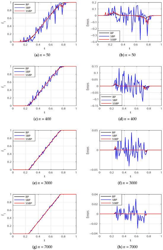
Figure 1. Pointwise approximation errors (to $f_1$) given by BPs, SBPs, and SSBPs in one trial.

In Figure 2, the horizontal axes represent the degrees of SBPs and SSBPs, while the vertical axes represent the probabilities of certain events occurring, which we will elaborate on below. When approximating $f_1$, we set the tolerance $ϵ=0.02$ and selected nine equally spaced points, denoted as $t_j$$(1\le j\le 9)$, from the interval $[0,1]$, starting from $t_1=0.1$. The total set of these points is denoted by $\mathsf{\Xi }$. At each point $t_j$, we ran 1000 trials and computed the probabilities of the events ${\displaystyle |B_n^X{f}_i(t_j)-f_i(t_j)|>ϵ}$ and ${\displaystyle |B_n^T{f}_i(t_j)-f_i(t_j)|>ϵ}$$(i=1,2)$.

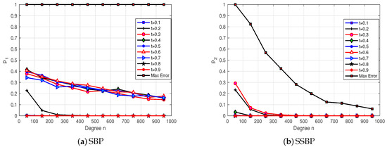
Figure 2. $f_1$: Simulations of probabilistic convergence of SBPs and SSBPs in 1000 trials.

Furthermore, we conducted 1000 trials to compute the probabilities of the events ${\displaystyle \underset{t_j\in \mathsf{\Xi }}{max}}|B_n^X{f}_i(t_j)-f_i(t_j)|>ϵ$ and ${\displaystyle \underset{t_j\in \mathsf{\Xi }}{max}}|B_n^T{f}_i(t_j)-f_i(t_j)|>ϵ$$(i=1,2)$. Figure 2 demonstrates that the probabilities of events associated with SSBPs decay exponentially as the polynomial degree n increases. In contrast, the probabilities of events associated with SBPs do not decay as rapidly as those for SSBPs.

5.2. Simulations of Normal Distribution Functions

In this subsection, we approximate another commonly used function, the normal density function:

$$f_2(x;\mu ,{\sigma }^2)={\displaystyle \frac{1}{\sqrt{2\pi {\sigma }^2}}}{e}^{-{\displaystyle \frac{{(x-\mu )}^2}{2{\sigma }^2}}},$$

(15)

where $\mu =0.5$, $\sigma =0.1$. The normal density function is widely applied, not only in probability theory but also in areas like kernel approximation, neural networks, and deep learning. Therefore, accurately approximating this function is of great importance. Although the function is infinitely smooth, it presents a challenge due to its significant curvature changes, which can lead to substantial errors if the approximation method is inadequate.

As shown in the Table 2 and Figure 3, the error obtained from the approximation using SSBPs is acceptable, while the error from SBPs becomes so large that it distorts the function’s shape. This demonstrates that SSBPs offer a superior approximation performance for this function. Figure 3 shows the approximation results for polynomial degrees $n=50,100,700,3000,5000,7000$, corresponding to the results summarized in Table 2.

Table 2. Maximal approximation errors given by BPs, SBPs, and SSBPs.

	n	50	100	400	1000	3000	5000	7000
$f_2$	BP	0.2860	0.1659	0.0469	0.0193	0.0065	0.0039	0.0021
	SBP	2.4255	1.8618	1.0705	1.0248	0.2801	0.2673	0.0239
	SSBP	0.7121	0.4584	0.1828	0.0561	0.0221	0.0212	0.0187

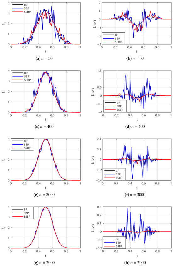
Figure 3. Pointwise approximation errors (to $f_2$) given by BPs, SBPs, and SSBPs in one trial.

In Figure 4, the horizontal axes represent the polynomial degrees for SBPs and SSBPs, while the vertical axes represent the probabilities of certain events occurring. Here, the specific event is defined as the approximation error exceeding 0.5. The probability of the error exceeding 0.5 decreases exponentially as n increases for SSBPs. In contrast, the probability associated with SBPs does not decay as rapidly. This indicates that SBPs are not as effective in approximating functions with large curvature variations, and their performance degrades further as the standard deviation of the normal density function increases.

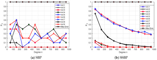
Figure 4. $f_2$: Simulations of probabilistic convergence of SBPs and SSBPs in 1000 trials.

Thus, we can observe that SSBPs are well-suited for approximating functions with large curvature changes, as the error remains manageable. From the comparison of these two very different functions—the uniform distribution and the normal density function—it becomes evident that SSBPs can handle noisy data effectively while providing approximation results comparable to classical BPs. Therefore, we conclude that SSBPs are highly reliable for these types of approximations.

6. Conclusions

This paper demonstrates the exponential convergence of SSBPs under the $L_p$ ($1\le p\le \infty$) norm. Theoretical analysis shows that the ${\omega }_2$-error bound of SSBPs is comparable to that of classical BPs and significantly outperforms the SBPs, while maintaining an $\mathcal{O}(N)$ computational complexity. It is worth mentioning that we establish probabilistic convergence rates for the general $L_p$ norm (Theorem 3), with explicit dependence on the parameter p. However, the numerical experiments in this study exclusively validate the $L_{\infty }$ and exponential convergence. While $L_{\infty }$ control provides a theoretical upper bound for $L_p$ errors, the actual convergence behavior for finite p values may exhibit distinct characteristics. Although the current study is limited to the univariate case, these findings provide new research directions for the field of stochastic computation, particularly in the extension to multivariate cases and the optimization of computational complexity, which are of significant exploratory value.

References

- Lin, D.; Johnson, P.; Knoll, F.; Lui, Y. Artificial intelligence for MR image reconstruction: An overview for clinicians. J. Magn. Reson. Imaging 2021, 53, 1015–1028. [Google Scholar] [CrossRef] [PubMed]
- Al-Quayed, F.; Ahmad, Z.; Humayun, M. A situation based predictive approach for cybersecurity intrusion detection and prevention using machine learning and deep learning algorithms in wireless sensor networks of industry 4.0. IEEE Access 2024, 12, 34800–34819. [Google Scholar] [CrossRef]
- El, Y.; Ellabib, A. A fuzzy particle swarm optimization method with application to shape design problem. RAIRO-Oper. Res. 2023, 57, 2819–2832. [Google Scholar]
- Lorentz, G. Bernstein Polynomials; American Mathematical Society: Providence, RI, USA, 2012. [Google Scholar]
- Cheney, E.W.; Light, W. A Course in Approximation Theory; American Mathematical Society: Providence, RI, USA, 2009; Volume 101. [Google Scholar]
- Ditzian, Z.; Totik, V. Moduli of Smoothness; Springer Science & Business Media: Berlin/Heidelberg, Germany, 2012; Volume 9. [Google Scholar]
- Chung, K. Elementary Probability Theory with Stochastic Processes; Springer Science & Business Media: Berlin/Heidelberg, Germany, 2012. [Google Scholar]
- Paltanea, R. Approximation Theory Using Positive Linear Operators; Springer Science & Business Media: Berlin/Heidelberg, Germany, 2012. [Google Scholar]
- Wu, Z.; Sun, X.; Ma, L. Sampling scattered data with Bernstein polynomials: Stochastic and deterministic error estimates. Adv. Comput. Math. 2013, 38, 187–205. [Google Scholar] [CrossRef]
- David, H.; Nagaraja, H. Order Statistics; John Wiley & Sons: Hoboken, NJ, USA, 2004. [Google Scholar]
- Sun, X.; Wu, Z. Chebyshev type inequality for stochastic Bernstein polynomials. Proc. Am. Math. Soc. 2019, 147, 671–679. [Google Scholar] [CrossRef]
- Sun, X.; Wu, Z.; Zhou, X. On probabilistic convergence rates of stochastic Bernstein polynomials. Math. Comput. 2021, 90, 813–830. [Google Scholar] [CrossRef]
- Sun, X.; Zhou, X. Stochastic Quasi-Interpolation with Bernstein Polynomials. Mediterr. J. Math. 2022, 19, 240. [Google Scholar] [CrossRef]
- Adell, J.; Cárdenas-Morales, D. Stochastic Bernstein polynomials: Uniform convergence in probability with rates. Adv. Comput. Math. 2020, 46, 16. [Google Scholar] [CrossRef]
- Adell, J.; Cárdenas-Morales, D. Random linear operators arising from piecewise linear interpolation on the unit interval. Mediterr. J. Math. 2022, 19, 223. [Google Scholar] [CrossRef]
- Adell, J.; Cárdenas-Morales, D.; López-Moreno, A. On the rates of pointwise convergence for Bernstein polynomials. Results Math. 2025, 80, 1–10. [Google Scholar] [CrossRef]
- Gao, W.; Sun, X.; Wu, Z.; Zhou, X. Multivariate Monte Carlo approximation based on scattered data. SIAM J. Sci. Comput 2020, 42, A2262–A2280. [Google Scholar] [CrossRef]
- Gao, W.; Fasshauer, G.; Sun, X.; Zhou, X. Optimality and regularization properties of quasi-interpolation: Deterministic and stochastic approaches. SIAM J. Numer. Anal. 2020, 58, 2059–2078. [Google Scholar] [CrossRef]
- Gal, S.; Niculescu, C. Approximation of random functions by stochastic Bernstein polynomials in capacity spaces. Carpathian J. Math. 2021, 37, 185–194. [Google Scholar] [CrossRef]
- Bouzebda, S. Uniform in number of neighbor consistency and weak convergence of k-nearest neighbor single index conditional processes and k-nearest neighbor single index conditional u-processes involving functional mixing data. Symmetry 2024, 16, 1576. [Google Scholar] [CrossRef]
- Cucker, F.; Smale, S. On the mathematical foundations of learning. Bull. Am. Math. Soc. 2002, 39, 1–49. [Google Scholar] [CrossRef]
- Cucker, F.; Zhou, D. Learning Theory: An Approximation Theory Viewpoint; Cambridge University Press: Cambridge, UK, 2007; Volume 24. [Google Scholar]
- Gao, Q.; Sun, X.; Zhang, S. Optimal stochastic Bernstein polynomials in Ditzian-Totik type modulus of smoothness. J. Comput. Appl. Math. 2022, 404, 113888. [Google Scholar] [CrossRef]
- Casella, G.; Berger, R. Statistical Inference; CRC Press: Boca Raton, FL, USA, 2024. [Google Scholar]
- Farin, G. Handbook of Computer Aided Geometric Design; Elsevier: Amsterdam, The Netherlands, 2002; Volume 2, pp. 577–580. [Google Scholar]
- Prautzsch, H.; Boehm, W.; Paluszny, M. Bézier and B-Spline Techniques; Springer Science & Business Media: Berlin/Heidelberg, Germany, 2002. [Google Scholar]
Disclaimer/Publisher’s Note: The statements, opinions and data contained in all publications are solely those of the individual author(s) and contributor(s) and not of MDPI and/or the editor(s). MDPI and/or the editor(s) disclaim responsibility for any injury to people or property resulting from any ideas, methods, instructions or products referred to in the content. |
© 2025 by the authors. Licensee MDPI, Basel, Switzerland. This article is an open access article distributed under the terms and conditions of the Creative Commons Attribution (CC BY) license (https://creativecommons.org/licenses/by/4.0/).