Dynamic Response Calculation of Inertial Coupled Nonlinear Systems Based on Real Modal Analysis and P-T Method

Abstract

The development of efficient and accurate numerical methods forms a crucial foundation for revealing complex dynamic evolution in nonlinear dynamical systems. Focusing on nonlinear inertia-coupled systems, this paper constructs a semi-analytical method that integrates the mathematical framework of real modal analysis with the piecewise constant arguments and Taylor series (P-T) method. This method first conducts symmetric preprocessing on the second-order term coefficient matrix of the system to construct the proportional damping decoupling form. Then, it realizes the linear term decoupling corresponding to this proportional damping form by using the mathematical framework of real modal analysis. Finally, the P-T method is applied to solve the dynamic response of the nonlinear system. Numerical validation using a two-dimensional aeroelastic system demonstrates that, under the premise of achieving the same computational accuracy as the time-domain minimum residual method (TMRM), the computational efficiency of the proposed method is significantly better than that of TMRM.

1. Introduction

Second-order differential equations, as extremely important research objects in the fields of mathematics and engineering, play an irreplaceable and crucial role in numerous areas such as physics, engineering, aerospace, etc. Their solution methods are diverse, including the analytical method for solving homogeneous equations through characteristic equations [1], the transformation method for simplifying the solution process with the help of the Laplace transform [2], the matrix method for multi-degree-of-freedom systems [3], and the perturbation method for handling nonlinear problems [4]. These methods provide researchers in related fields with a theoretical basis from theoretical derivation to practical application.

In nonlinear dynamics, many practical problems are expressed by second-order differential equations. However, solving some complex second-order differential equations is quite challenging, especially for systems of second-order nonlinear inertially coupled differential equations. Such systems typically do not have analytical solutions and can only be solved using various methods to obtain approximate or numerical solutions. Therefore, it is essential to find high-precision numerical methods. The P-T method, as a semi-analytical method, can theoretically improve the efficiency of solving second-order nonlinear inertial coupled differential equation systems. The P-T method is a semi-analytical method for solving linear and nonlinear oscillation systems in engineering dynamics [5]. Unlike the discrete solutions obtained by the existing numerical methods [6], the solutions obtained by the P-T method are continuous throughout the time domain. Most importantly, compared with the Runge–Kutta method [7] and other numerical methods for discrete solutions, the P-T method retains the physical intuitiveness of the vibration system. The P-T method, which serves as an important new method for obtaining approximate and numerical solutions of nonlinear vibration systems, began its research in this field in the early 1980s. The P-T method combines piecewise constant parameters and Taylor expansion solutions. Early research focused primarily on the application of piecewise constants. Initially, piecewise constants were used to find stable regions for time-delay differential equations [8], and the existence and uniqueness theorems of their solutions were proved [9]. Subsequently, analytical and numerical methods for solving linear and nonlinear vibration problems with piecewise constant parameters were introduced, and continuous solutions were obtained [10,11,12,13,14,15,16]. With the in-depth research of nonlinear dynamics, Dai and Singh [17] proposed a new method, the P-T method, in order to further improve the numerical calculation efficiency based on piecewise constant technology, combined with Taylor series, for solving common linear and nonlinear vibration systems in engineering dynamics. Based on this, Dai studied the accuracy and reliability of the numerical simulation of nonlinear dynamical systems through the Runge–Kutta method and the P-T method [18].

The above content introduces the development background of the P-T method. Based on the current research progress in the field of inertially coupled vibrations, Dai proposed a new segmented Laplace method to solve second-order linear inertially coupled differential equation systems [19]. This method solves inertially coupled linear vibration problems while retaining the inertial term, and makes the solution continuous throughout the entire time domain. However, to date, this research has not been applied to nonlinear systems. Based on this, this paper constructs a structure that satisfies the mathematical form of proportional damping through the mathematical framework of real mode analysis to achieve decoupling, thereby retaining the inertial term, and obtains the continuous solution of the inertially coupled nonlinear system through the P-T method.

Real modal analysis has been studied both at home and abroad. It is an effective method to simplify multi-degree-of-freedom vibration systems, but it usually relies on proportional damping. In order to solve the non-proportional damping system, the components in the system equation that satisfy the mathematical form of proportional damping can be separated to the left side of the equal sign, while the remaining terms are moved to the right side of the equal sign, and the P-T method is adopted for solution.

According to the literature reviewed by the author, no research has been found so far to construct a structure that satisfies the decoupled form of proportional damping by using the mathematical process of real modal analysis while retaining the inertial term, and to apply the P-T method to non-proportional damping systems in combination. Therefore, combining the P-T method with real modal analysis and applying it to the dynamic study of inertially coupled nonlinear vibration systems has significant research significance.

2. Fundamental Theory

2.1. Mathematical Theory Derivation of Real Modal Decoupling

This paper adopts the mathematical process of real modal analysis as the basic tool to achieve the decoupling of the inertial coupling nonlinear vibration equation. This method is based on the conventional dynamic condition that the mass matrix M and the stiffness matrix K are positive definite matrices. Firstly, by introducing preprocessing methods such as scaling factors, the symmetry of the second-order term coefficient matrix is achieved. Then, by shifting terms, the left side of the equation satisfies the proportional damping form of $\mathbf{C}=\alpha \mathbf{M}+\beta \mathbf{K}$, creating conditions for decoupling. On this basis, the generalized eigenvalue decomposition and orthogonal transformation in the mathematical framework of real mode analysis are utilized to achieve mathematical decoupling on the left side of the equation. The terms such as “real modal analysis”, “proportional damping”, “modal coordinates”, and “eigenvalues” that appear in the text, as symbols and conceptual systems describing the above mathematical process, represent mathematical operations and intermediate variables, and do not involve the interpretation of physical characteristics such as the natural frequency and mode shape of the system. The ultimate goal of this paper is to construct a decoupled mathematical form, laying the foundation for the subsequent solution using the P-T method.

Many complex dynamical systems are often described by second-order nonlinear differential equations, and the solution of their dynamic responses relies on computer numerical methods. The development of numerical methods that are both highly accurate and efficient is of crucial significance for enhancing the reliability and computational efficiency of dynamic analysis in complex systems. In the field of vibration engineering, the dynamic [20,21,22,23,24] responses of systems such as mechanical structures, aerospace components, and precision instruments involve significant nonlinear dynamic behaviors. To accurately describe the dynamic characteristics of such complex systems, their general form can be expressed as the following second-order nonlinear coupled differential equations:

$$\left\{\begin{array}{c}{a}_1{x_1}^{″}+a_2{x_2}^{″}+{\mathrm{b}}_1{x_1}^{\prime }+{\mathrm{b}}_2{x_2}^{\prime }+d_1{x}_1+d_2{x}_2+f(x_1,x_2,{x_1}^{\prime },{x_2}^{\prime })=f_1(t)\\ a_3{x_1}^{″}+a_4{x_2}^{″}+{\mathrm{b}}_3{x_1}^{\prime }+{\mathrm{b}}_4{x_2}^{\prime }+d_3{x}_1+d_4{x}_2+g(x_1,x_2,{x_1}^{\prime },{x_2}^{\prime })=f_2(t)\end{array}\right.$$

(1)

Among them, $a_i,{\mathrm{b}}_i$, and $d_i(i=1,2,3,4)$ are the system parameters, $f(x_1,x_2,{x_1}^{\prime },{x_2}^{\prime })$ and $g(x_1,x_2,{x_1}^{\prime },{x_2}^{\prime })$ are nonlinear coupling terms, and $f_1(t)$ and $f_2(t)$ are linear or nonlinear terms related to time, displacement, and oscillator velocity. Since real modal analysis requires the system’s inertia matrix to be symmetric, when the inertia matrix is not symmetric, we can multiply each equation of the original system by a specific scaling factor. This transforms it into an equivalent form with a symmetric inertia matrix, thereby creating the conditions for applying real modal analysis. When the inertia matrix $\left[\begin{array}{cc}{a}_1& a_2\\ a_3& a_4\end{array}\right]$ is a nonsymmetric matrix, the least common multiple of $a_2,a_3$ is $LCM(a_2,a_3)$. Perform block scaling transformation on the equation system with asymmetric mass matrix in Equation (1), apply $LCM(a_2,a_3)/a_2=1/h_1$ scaling to the upper equation and $LCM(a_2,a_3)/a_3=1/h_2$ scaling to the lower equation, thereby converting the mass matrix into a symmetric form

$$\left\{\begin{array}{c}\begin{array}{l}{\displaystyle \frac{a_1{x_1}^{″}}{h_1}}+LCM(a_2,a_3){x_2}^{″}+{\displaystyle \frac{{\mathrm{b}}_1{x_1}^{\prime }}{h_1}}+{\displaystyle \frac{{\mathrm{b}}_2{x_2}^{\prime }}{h_1}}+{\displaystyle \frac{d_1{x}_1}{h_1}}+{\displaystyle \frac{d_2{x}_2}{h_1}}+{\displaystyle \frac{f(x_1,x_2,{x_1}^{\prime },{x_2}^{\prime })}{h_1}}={\displaystyle \frac{f_1(t)}{h_1}}\\ =m_1{x_1}^{″}+m_2{x_2}^{″}+{\mathrm{c}}_1{x_1}^{\prime }+{\mathrm{c}}_2{x_2}^{\prime }+k_1{x}_1+k_2{x}_2+f_{nl}(x_1,x_2,{x_1}^{\prime },{x_2}^{\prime })=F_1(t)\end{array}\\ \begin{array}{l}LCM(a_2,a_3){x_1}^{″}+{\displaystyle \frac{a_4{x_2}^{″}}{h_2}}+{\displaystyle \frac{{\mathrm{b}}_3{x_1}^{\prime }}{h_2}}+{\displaystyle \frac{{\mathrm{b}}_4{x_2}^{\prime }}{h_2}}+{\displaystyle \frac{d_3{x}_1}{h_2}}+{\displaystyle \frac{d_4{x}_2}{h_2}}+{\displaystyle \frac{g(x_1,x_2,{x_1}^{\prime },{x_2}^{\prime })}{h_2}}={\displaystyle \frac{f_2(t)}{h_2}}\\ =m_3{x_1}^{″}+m_4{x_2}^{″}+{\mathrm{c}}_3{x_1}^{\prime }+{\mathrm{c}}_4{x_2}^{\prime }+k_3{x}_1+k_4{x}_2+g_{nl}(x_1,x_2,{x_1}^{\prime },{x_2}^{\prime })=F_2(t)\end{array}\end{array}\right.$$

(2)

If the inertia matrix $\left[\begin{array}{cc}{a}_1& a_2\\ a_3& a_4\end{array}\right]$ is a symmetric matrix, no transformation is required. The original equation of the inertial symmetric system and the transformed equation of the inertial symmetric system are uniformly expressed as

$$\left\{\begin{array}{c}{m}_1{x_1}^{″}+m_2{x_2}^{″}+{\mathrm{c}}_1{x_1}^{\prime }+{\mathrm{c}}_2{x_2}^{\prime }+k_1{x}_1+k_2{x}_2+f_{nl}(x_1,x_2,{x_1}^{\prime },{x_2}^{\prime })=F_1(t)\\ m_3{x_1}^{″}+m_4{x_2}^{″}+{\mathrm{c}}_3{x_1}^{\prime }+{\mathrm{c}}_4{x_2}^{\prime }+k_3{x}_1+k_4{x}_2+g_{nl}(x_1,x_2,{x_1}^{\prime },{x_2}^{\prime })=F_2(t)\end{array}\right.$$

(3)

We further simplify Equation (3) into a matrix form.

$$M{x}^{″}(t)+C{x}^{\prime }(t)+Kx(t)=F(t)-G_{nl}(t)$$

(4)

Then, $M=\left[\begin{array}{cc}{m}_1& m_2\\ m_2& m_3\end{array}\right]$ is the mass matrix, $C=\left[\begin{array}{cc}{\mathrm{c}}_1& {\mathrm{c}}_2\\ {\mathrm{c}}_3& {\mathrm{c}}_4\end{array}\right]$ is the damping matrix, $K=\left[\begin{array}{cc}{k}_1& k_2\\ k_3& k_4\end{array}\right]$ is the stiffness matrix, $G_{nl}(t)=\left[\begin{array}{c}{f}_{nl}(x_1,x_2,{x_1}^{\prime },{x_2}^{\prime })\\ g_{nl}(x_1,x_2,{x_1}^{\prime },{x_2}^{\prime })\end{array}\right]$ is the coupling term matrix, $F(t)=\left[\begin{array}{c}{F}_1(t)\\ F_2(t)\end{array}\right]$ is the matrix related to time, displacement, and oscillator velocity, and $x(t)$ is the displacement vector. Make the coefficients on the left side of the equation satisfy the proportional damping mathematical form of $C=\alpha M+\beta K$ ($\alpha \ge 0,\beta \ge 0$) to achieve decoupling on the left side. The right side contains the remaining linear and nonlinear terms. To decouple the system, we first ignore $F(t)-G_{nl}(t)$ and damping, setting $C=0$ and $F(t)-G_{nl}(t)=0$. The system can be expressed in terms of mass and stiffness as:

$$M{x}^{″}(t)+Kx(t)=0$$

(5)

Suppose the solution of the system is in the form of a simple harmonic vibration $x(t)={\mathit{\varphi }}_k{e}^{i{w}_{k}t}$, where ${\mathit{\varphi }}_k$ is a vector. Substituting it into Equation (5), the generalized characteristic equation is obtained:

$$K{\mathit{\varphi }}_k={w_k}^{2}M{\mathit{\varphi }}_k$$

(6)

Convert vector $x(t)$ into modal coordinate vector $q(t)$:

$$x(t)=\Phi q(t)$$

(7)

where $\Phi$ is the modal matrix, substituting Equation (7) into the original set of equations and multiplying by ${\Phi }^T$ on the left, we obtain:

$${\Phi }^{T}M\Phi q^{″}(t)+{\Phi }^{T}C\Phi q^{\prime }(t)+{\Phi }^{T}K\Phi q(t)={\Phi }^T(F(t)-G_{nl}(t))$$

(8)

From the modal orthogonality of symmetric systems and reference [25], it can be known that in the generalized eigenvalue problem involving two symmetric matrices $M$ and $K$, if $M$ and $K$ are symmetric positive definite matrices, then the modal shapes are orthogonal concerning $M$ and $K$:

$${\Phi }^{T}M\Phi =\delta ,{\Phi }^{T}K\Phi ={\Phi }^T{w_k}^{2}M\Phi ={w_k}^2\delta$$

(9)

We perform quality normalization on the real mode so that:

$${\Phi }^{T}M\Phi =I,{\Phi }^{T}K\Phi ={\Omega }^2,{\Omega }^2=diag({w_1}^2,{w_2}^2)$$

(10)

Suppose the damping matrix $C$ satisfies proportional damping.

$$C=\alpha M+\beta K$$

(11)

Since $M$, $K$ is a symmetric matrix, $C$ is also a symmetric matrix. Substituting Equation (11) into ${\Phi }^{T}C\Phi$ gives:

$${\Phi }^{T}C\Phi ={\Phi }^T(\alpha M+\beta K)\Phi =\alpha I+\beta {\Omega }^2=diag(\alpha +\beta w_1^2,\alpha +\beta w_2^2)$$

(12)

From Equation (12), it is known that when $C$ satisfies proportional damping, ${\Phi }^{T}C\Phi$ is a diagonal matrix. Substitute the original system of equations and express it as:

$$\begin{array}{l}{q^{″}}_i(t)+(\alpha +\beta w_k^2){q^{\prime }}_i(t)+w_k^2{q}_i(t)={\Phi }^T\left(\begin{array}{c}{F}_1(t)-f_{nl}(x_1,x_2,{x_1}^{\prime },{x_2}^{\prime })\\ F_2(t)-g_{nl}(x_1,x_2,{x_1}^{\prime },{x_2}^{\prime })\end{array}\right)\end{array}$$

(13)

In this way, the left equation can be decoupled. Substituting $x(t)=\Phi q(t)$ on the right side of the equal sign in Equation (13) can transform the entire equation into an expression of $q(t)$.

2.2. The Theoretical Basis of the P-T Method

The equations of the multi-degree-of-freedom vibration system obtained from Section 2.1 are abbreviated as follows:

$$\left\{\begin{array}{c}{q^{″}}_1(t)+(\alpha +\beta w_1^2){q^{\prime }}_1(t)+w_1^2{q}_1(t)=g_1(t,q_1,q_2,{q_1}^{\prime },{q_2}^{\prime })\\ {q^{″}}_2(t)+(\alpha +\beta w_2^2){q^{\prime }}_2(t)+w_2^2{q}_2(t)=g_2(t,q_1,q_2,{q_1}^{\prime },{q_2}^{\prime })\end{array}\right.$$

(14)

Among them, $\alpha +\beta w_k^2$ and $w_k^2(k=1,2)$ are parameters obtained after decoupling the system described in Equation (1), and $g_k(t,q_1,q_2,{q_1}^{\prime },{q_2}^{\prime })$ is a function related to time, displacement, and oscillator velocity. This method was proposed by Dai and Singh [10] for addressing linear and nonlinear vibration problems. The core lies in dividing the entire time domain into $N$ sub-intervals of length ${\displaystyle \frac{1}{N}}$ by introducing a piecewise constant parameter ${\displaystyle \frac{\left[Nt\right]}{N}}$ (where $\left[Nt\right]$ represents the rounding down function and $N$ is an integer parameter). Within each sub-interval ${\displaystyle \frac{\left[Nt\right]}{N}}\le t<{\displaystyle \frac{\left[Nt\right]+1}{N}}$, the original equation is transformed into a linear ordinary differential equation with constant coefficients through Taylor series expansion. This type of equation has analytical solutions, which are continuous within the sub-intervals. By adding the continuity conditions $q_{k_i}({\displaystyle \frac{\left[Nt\right]}{N}})=q_{k_{i-1}}({\displaystyle \frac{\left[Nt\right]}{N}})$, $q_{k_i}({\displaystyle \frac{\left[Nt\right]}{N}}{)}^{\prime }=q_{k_{i-1}}({\displaystyle \frac{\left[Nt\right]}{N}}{)}^{\prime }$, it is ensured that the solutions are continuous at the connection points, and ultimately, a continuous solution for the entire time domain is obtained. Parameter $N$ is used to control the length of the time interval and the accuracy of the calculation. When $N$ approaches infinity, the numerical solution of the piecewise system converges to the solution of the original continuous system in the time domain, thereby obtaining a continuous Semi-analytical solution. Dai and Singh [17] have mathematically proven:

Theorem 1.

Suppose $\left[Nt\right]$is a maximum integer function related to$t$and$N$, where N is a positive integer. Then, as$N$approaches infinity, the ratio${\displaystyle \frac{\left[Nt\right]}{N}}$approaches$t$.

$$\underset{N\to \infty }{\lim }{\displaystyle \frac{\left[Nt\right]}{N}}=t$$

(15)

To simplify the calculation, linearize the equation for each time interval. Expand the control equation using Taylor’s formula at the $i$th time interval ${\displaystyle \frac{\left[Nt\right]}{N}}\le t<{\displaystyle \frac{\left[Nt\right]+1}{N}}$, keeping the linear terms unchanged.

To further enhance the numerical calculation efficiency based on the piecewise constant method, A Taylor series is adopted to expand at point $t={\displaystyle \frac{[Nt]}{N}}$.

$$\left\{\begin{array}{c}\begin{array}{l}{g}_1(t,q_1,q_2,{q_1}^{\prime },{q_2}^{\prime })=g_{1_{{\displaystyle \frac{\left[Nt\right]}{N}}}}+{g_{1_{{\displaystyle \frac{\left[Nt\right]}{N}}}}}^{\prime }\left(t-{\displaystyle \frac{[Nt]}{N}}\right)+{\displaystyle \frac{1}{2!}}{g_{1_{{\displaystyle \frac{\left[Nt\right]}{N}}}}}^{″}{\left(t-{\displaystyle \frac{[Nt]}{N}}\right)}^2\\ +\cdots +{\displaystyle \frac{1}{n!}}{g_{1_{{\displaystyle \frac{\left[Nt\right]}{N}}}}}^{(n)}{\left(t-{\displaystyle \frac{[Nt]}{N}}\right)}^n+R_{n_1}(x)\end{array}\\ \begin{array}{l}{g}_2(t,q_1,q_2,{q_1}^{\prime },{q_2}^{\prime })=g_{2_{{\displaystyle \frac{\left[Nt\right]}{N}}}}+{g_{2_{{\displaystyle \frac{\left[Nt\right]}{N}}}}}^{\prime }\left(t-{\displaystyle \frac{[Nt]}{N}}\right)+{\displaystyle \frac{1}{2!}}{g_{2_{{\displaystyle \frac{\left[Nt\right]}{N}}}}}^{″}{\left(t-{\displaystyle \frac{[Nt]}{N}}\right)}^2\\ +\cdots +{\displaystyle \frac{1}{n!}}{g_{2_{{\displaystyle \frac{\left[Nt\right]}{N}}}}}^{(n)}{\left(t-{\displaystyle \frac{[Nt]}{N}}\right)}^n+R_{n_2}(x)\end{array}\end{array}\right.$$

(16)

Reference [17] has demonstrated that, when $\left|t-{\displaystyle \frac{\left[Nt\right]}{N}}\right|\le {\displaystyle \frac{1}{N}}$ and $N\to \infty$ are satisfied, the truncation error $R_{n_k}\to 0$ holds, and the conclusions ${q^{″}}_k({\displaystyle \frac{[Nt]}{N}})\to {q^{″}}_k(t)$,${q^{\prime }}_k({\displaystyle \frac{[Nt]}{N}})\to {q^{\prime }}_k(t)$,$q_k({\displaystyle \frac{[Nt]}{N}})\to q_k(t)$ and $g_k({\displaystyle \frac{[Nt]}{N}},q_1({\displaystyle \frac{[Nt]}{N}}),q_2({\displaystyle \frac{[Nt]}{N}}),{q_1}^{\prime }({\displaystyle \frac{[Nt]}{N}}),{q_2}^{\prime }({\displaystyle \frac{[Nt]}{N}}))$$\to g_k(t,q_1,q_2,{q_1}^{\prime },{q_2}^{\prime })$ are valid. The function value and derivative value of function $g_k(t,q_1,q_2,{q_1}^{\prime },{q_2}^{\prime })$ at point $t={\displaystyle \frac{\left[Nt\right]}{N}}$ are as follows:

$$\begin{array}{l}{g_k}_{{\displaystyle \frac{\left[Nt\right]}{N}}}=g_k({\displaystyle \frac{[Nt]}{N}},q_{1_i}({\displaystyle \frac{[Nt]}{N}}),q_{2_i}({\displaystyle \frac{[Nt]}{N}}),{q_{1_i}}^{\prime }({\displaystyle \frac{[Nt]}{N}}),{q_{2_i}}^{\prime }({\displaystyle \frac{[Nt]}{N}}))\\ {{g_k}_{{\displaystyle \frac{\left[Nt\right]}{N}}}}^{\prime }={\left[{\displaystyle \frac{d}{dt}}{g}_k(t,q_{1_i},q_{2_i},{q_{1_i}}^{\prime },{q_{2_i}}^{\prime })\right]}_{t={\displaystyle \frac{\left[Nt\right]}{N}}}\\ {{g_k}_{{\displaystyle \frac{\left[Nt\right]}{N}}}}^{″}={\left[{\displaystyle \frac{d^2}{d{t}^2}}{g}_k(t,q_{1_i},q_{2_i},{q_{1_i}}^{\prime },{q_{2_i}}^{\prime })\right]}_{t={\displaystyle \frac{\left[Nt\right]}{N}}}\\ ⋮\\ {{g_k}_{{\displaystyle \frac{\left[Nt\right]}{N}}}}^{\left(n\right)}={\left[{\displaystyle \frac{d^n}{d{t}^n}}{g}_k(t,q_{1_i},q_{2_i},{q_{1_i}}^{\prime },{q_2}^{\prime })\right]}_{t={\displaystyle \frac{\left[Nt\right]}{N}}}\end{array}$$

(17)

Since the commonly used numerical method for solving nonlinear problems is the 4th-order Runge–Kutta method, the 4th-order P-T method can be used here, with the higher-order terms truncated after Taylor expansion.

$$\left\{\begin{array}{c}\begin{array}{l}{q^{″}}_1(t)+(\alpha +\beta w_1^2){q^{\prime }}_1(t)+w_1^2{q}_1(t)={g_1}_{{\displaystyle \frac{\left[Nt\right]}{N}}}+{{g_1}_{{\displaystyle \frac{\left[Nt\right]}{N}}}}^{\prime }\left(t-{\displaystyle \frac{[Nt]}{N}}\right)+{\displaystyle \frac{1}{2!}}{{g_1}_{{\displaystyle \frac{\left[Nt\right]}{N}}}}^{″}{\left(t-{\displaystyle \frac{[Nt]}{N}}\right)}^2\\ +{\displaystyle \frac{1}{3!}}{{g_1}_{{\displaystyle \frac{\left[Nt\right]}{N}}}}^{‴}{\left(t-{\displaystyle \frac{[Nt]}{N}}\right)}^3\end{array}\\ \begin{array}{l}{q^{″}}_2(t)+(\alpha +\beta w_2^2){q^{\prime }}_2(t)+w_2^2{q}_2(t)={g_2}_{{\displaystyle \frac{\left[Nt\right]}{N}}}+{{g_2}_{{\displaystyle \frac{\left[Nt\right]}{N}}}}^{\prime }\left(t-{\displaystyle \frac{[Nt]}{N}}\right)+{\displaystyle \frac{1}{2!}}{{g_2}_{{\displaystyle \frac{\left[Nt\right]}{N}}}}^{″}{\left(t-{\displaystyle \frac{[Nt]}{N}}\right)}^2\\ +{\displaystyle \frac{1}{3!}}{{g_2}_{{\displaystyle \frac{\left[Nt\right]}{N}}}}^{‴}{\left(t-{\displaystyle \frac{[Nt]}{N}}\right)}^3\end{array}\end{array}\right.$$

(18)

In time interval $i=\left[Nt\right]$, the local initial conditions are as follows:

$$\begin{array}{l}{q}_{k_i}({\displaystyle \frac{\left[Nt\right]}{N}})=d_{k_i}\\ {q_{k_i}}^{\prime }({\displaystyle \frac{\left[Nt\right]}{N}})=v_{k_i}\end{array}$$

(19)

The solution within the $i$th time interval is generated using the 4th-order P-T method as follows:

$$\left\{\begin{array}{c}\begin{array}{l}{q}_1=e^{-{\displaystyle \frac{\alpha +\beta w_1^2}{2}}(t-{\displaystyle \frac{[Nt]}{N}})}\left\{B_{11}\cos \left[h_1\left(t-{\displaystyle \frac{[Nt]}{N}}\right)\right]+B_{12}\sin \left[h_1\left(t-{\displaystyle \frac{[Nt]}{N}}\right)\right]\right\}+A_{11}\\ +A_{12}\left(t-{\displaystyle \frac{[Nt]}{N}}\right)+A_{13}{\left(t-{\displaystyle \frac{[Nt]}{N}}\right)}^2+A_{14}\left(t-{\displaystyle \frac{[Nt]}{N}}\right)\end{array}\\ \begin{array}{l}{q}_2=e^{-{\displaystyle \frac{\alpha +\beta w_2^2}{2}}(t-{\displaystyle \frac{[Nt]}{N}})}\left\{B_{21}\cos \left[h_2\left(t-{\displaystyle \frac{[Nt]}{N}}\right)\right]+B_{22}\sin \left[h_2\left(t-{\displaystyle \frac{[Nt]}{N}}\right)\right]\right\}+A_{21}\\ +A_{22}\left(t-{\displaystyle \frac{[Nt]}{N}}\right)+A_{23}{\left(t-{\displaystyle \frac{[Nt]}{N}}\right)}^2+A_{24}\left(t-{\displaystyle \frac{[Nt]}{N}}\right)\end{array}\end{array}\right.$$

(20)

Among them

$$\begin{gathered} \begin{array}{l}{h_1}^2=w_1^2-{\displaystyle \frac{{(\alpha +\beta w_1^2)}^2}{4}}\\ {h_2}^2=w_2^2-{\displaystyle \frac{{(\alpha +\beta w_2^2)}^2}{4}}\\ A_{14}={\displaystyle \frac{1}{6w_1^2}}{{g_1}_{{\displaystyle \frac{\left[Nt\right]}{N}}}}^{‴}\\ A_{24}={\displaystyle \frac{1}{6w_2^2}}{{g_2}_{{\displaystyle \frac{\left[Nt\right]}{N}}}}^{‴}\end{array} \\ \begin{array}{l}{A}_{13}={\displaystyle \frac{1}{w_1^2}}({\displaystyle \frac{1}{2}}{{g_1}_{{\displaystyle \frac{\left[Nt\right]}{N}}}}^{″}-3(\alpha +\beta w_1^2)A_{14})\\ A_{23}={\displaystyle \frac{1}{w_2^2}}({\displaystyle \frac{1}{2}}{{g_2}_{{\displaystyle \frac{\left[Nt\right]}{N}}}}^{″}-3(\alpha +\beta w_2^2)A_{24})\\ A_{12}={\displaystyle \frac{1}{w_1^2}}\left({{g_1}_{{\displaystyle \frac{\left[Nt\right]}{N}}}}^{\prime }-2(\alpha +\beta w_1^2)A_{13}-6A_{14}\right)\\ A_{22}={\displaystyle \frac{1}{w_2^2}}\left({{g_2}_{{\displaystyle \frac{\left[Nt\right]}{N}}}}^{\prime }-2(\alpha +\beta w_2^2)A_{23}-6A_{24}\right)\\ A_{11}={\displaystyle \frac{1}{w_1^2}}\left({g_1}_{{\displaystyle \frac{\left[Nt\right]}{N}}}-(\alpha +\beta w_1^2)A_{12}-2A_{13}\right)\\ A_{21}={\displaystyle \frac{1}{w_2^2}}\left({g_2}_{{\displaystyle \frac{\left[Nt\right]}{N}}}-(\alpha +\beta w_2^2)A_{22}-2A_{23}\right)\\ B_{11}=d_{1_i}-A_{11}\\ B_{21}=d_{2_i}-A_{21}\\ B_{12}={\displaystyle \frac{1}{h_1}}(v_{1_i}+{\displaystyle \frac{\alpha +\beta w_1^2}{2}}{B}_{11}-A_{12})\\ B_{22}={\displaystyle \frac{1}{h_2}}(v_{2_i}+{\displaystyle \frac{\alpha +\beta w_2^2}{2}}{B}_{21}-A_{22})\end{array} \end{gathered}$$

(21)

The function is continuous in the interval ${\displaystyle \frac{\left[Nt\right]}{N}}\le t<{\displaystyle \frac{\left[Nt\right]+1}{N}}$, so it must satisfy:

$$\begin{array}{l}{q}_{k_i}({\displaystyle \frac{\left[Nt\right]}{N}})=q_{k_{i-1}}({\displaystyle \frac{\left[Nt\right]}{N}})\\ q_{k_i}({\displaystyle \frac{\left[Nt\right]}{N}}{)}^{\prime }=q_{k_{i-1}}({\displaystyle \frac{\left[Nt\right]}{N}}{)}^{\prime }\end{array}$$

(22)

Based on the above recursive relationship, the dynamic response of the system can be solved through numerical iterative algorithms.

3. Algorithm Application and Verification

3.1. Inertial Symmetric Coupled Nonlinear Vibration System

The interaction of the mass term in inertially coupled nonlinear systems makes it difficult to obtain an analytical solution directly, which makes its solution difficulty far exceed that of traditional dynamic equations. For this difficult problem, in this paper, real modal analysis combined with the P-T method is adopted to effectively solve the problem of the inertially coupled nonlinear system, and the effectiveness of this method is verified through the two-dimensional airfoil vibration model. The two-dimensional airfoil vibration model features inertial coupling and nonlinear characteristics. The dynamic behaviors of the system, such as bifurcation and limit loop oscillation, have been widely studied, providing a sufficient benchmark for method validation. For the inertially symmetric coupled nonlinear vibration problem, the classical model of two-dimensional wing flutter can be adopted for description [26]:

$$\left\{\begin{array}{ll}u{\xi }^{″}+u{\chi }_a{a}^{″}+{\displaystyle \frac{c_{\xi }}{\pi \rho b^2{\omega }_a}}{\xi }^{\prime }+u{({\displaystyle \frac{{\omega }_{\xi }}{{\omega }_a}})}^2{\displaystyle \frac{\mathit{\partial }V}{\mathit{\partial }\xi }}=-2{({\displaystyle \frac{V}{b{\omega }_a}})}^{2}a\hfill & \hfill \\ u{\chi }_a{\xi }^{″}+u{r}_a^2{a}^{″}+{\displaystyle \frac{c_a}{\pi \rho b^2{\omega }_a}}{a}^{\prime }+u{r}_a^{2}a{\displaystyle \frac{\mathit{\partial }V}{\mathit{\partial }a}}=(1+2a_h){({\displaystyle \frac{V}{b{\omega }_a}})}^{2}a\hfill & \hfill \end{array}\right.$$

(23)

Among them, $\xi$ is the vertical displacement, $a$ is the rotation Angle, $V={\displaystyle \frac{1}{2}}{\xi }^2+{\displaystyle \frac{1}{2}}{a}^2+{\displaystyle \frac{1}{4}}{\delta }_3{a}^4$ is the flow velocity, and the dimensionless flow velocity $Q={({\displaystyle \frac{V}{b{\omega }_a}})}^2$ is introduced. Other parameters are taken from reference [27], $u=20$, ${\chi }_a=0.25$, ${\omega }_a=62.8Hz$, $b=1m$, $r_a^2=0.5$, ${({\displaystyle \frac{{\omega }_{\xi }}{{\omega }_a}})}^2=0.2$, and $a_h=-0.1$, and we obtain:

$$\left\{\begin{array}{ll}{\xi }^{″}+0.25a^{″}+0.1{\xi }^{\prime }+0.2\xi +0.1Qa=0\hfill & \hfill \\ 0.25{\xi }^{″}+0.5a^{″}+0.1a^{\prime }+0.04Qa+f(a)=0\hfill & \hfill \end{array}\right.$$

(24)

Suppose the rotation Angle $a$ of the system has a cubic nonlinear term, then $f(a)=r_a^2(a+{\delta }_3{a}^3)$, $Q=8$, the system equation is written as:

$$\left\{\begin{array}{ll}{\xi }^{″}+0.25a^{″}+0.1{\xi }^{\prime }+0.2\xi +0.8a=0\hfill & \hfill \\ 0.25{\xi }^{″}+0.5a^{″}+0.1a^{\prime }+0.18a+20a^3=0\hfill & \hfill \end{array}\right.$$

(25)

Equation (25) represents an inertially coupled nonlinear vibration system. Decoupling of coupled problems often employs real modal analysis. From the derivation in Section 2.1, it is known that the conditions for applying real modal analysis are that $M$ and $K$ are symmetric positive definite matrices, the damping matrix $C$ is a $C=\alpha M+\beta K$ symmetric matrix, and the proportional damping a is satisfied. Therefore, to construct a system matrix suitable for real-mode analysis, it is necessary to first construct the left side of the equation into a structure that satisfies the form of proportional damping, and any redundant terms generated during the construction process should be moved to the right-hand side of the equation. In addition, we must minimize the differences between the coefficients $M$, $K$ and $C$ on the left side of the equals sign and the coefficients of the corresponding terms in the original equation as much as possible. This is because the P-T method uses Taylor series expansion for the right-hand side of the equation, and larger differences on the left-hand side result in greater errors. Since Equation (25) does not satisfy proportional damping $C\ne \alpha M+\beta K$, the proportional damping is constructed as follows:

$$\left\{\begin{array}{ll}{\xi }^{″}+0.25a^{″}+0.1{\xi }^{\prime }+0.2\xi =-0.8a\hfill & \hfill \\ 0.25{\xi }^{″}+0.5a^{″}+0.1a^{\prime }+0.2a=0.02a-20a^3\hfill & \hfill \end{array}\right.$$

(26)

Among them,

$$M=\left[\begin{array}{cc}1& 0.25\\ 0.25& 0.5\end{array}\right],C=\left[\begin{array}{cc}0.1& 0\\ 0& 0.1\end{array}\right],K=\left[\begin{array}{cc}0.2& 0\\ 0& 0.2\end{array}\right],C=0\times M+0.5\times K$$

(27)

The structure of Equation (27) satisfies the conditions for the real modal analysis. Ignoring the expression on the right-hand side of Equation (26), decouple Equation (28):

$$\left\{\begin{array}{ll}{\xi }^{″}+0.25a^{″}+0.1{\xi }^{\prime }+0.2\xi =0\hfill & \hfill \\ 0.25{\xi }^{″}+0.5a^{″}+0.1a^{\prime }+0.2a=0\hfill & \hfill \end{array}\right.$$

(28)

Based on the modal orthogonality of the symmetric system, the modal coordinate transformation $\xi ={\mathit{\varphi }}_1{q}_1,\mathit{a}={\mathit{\varphi }}_2{q}_2$ is carried out, and the characteristic equation $(K-\lambda M)\mathit{\varphi }=0$ of the generalized eigenvalue problem is solved to obtain the modal matrix:

$$\Phi =\left[\begin{array}{cc}1& 1\\ -{\displaystyle \frac{5+4\sqrt{2}}{3+\sqrt{2}}}& {\displaystyle \frac{-5+4\sqrt{2}}{3-\sqrt{2}}}\end{array}\right]$$

(29)

To obtain ${\Phi }^{T}M\Phi =I$, normalize $\Phi$:

$$\Phi =\left[\begin{array}{cc}{\displaystyle \frac{1}{1.6453}}& {\displaystyle \frac{1}{1.137}}\\ -{\displaystyle \frac{5+4\sqrt{2}}{4.9359+1.6453\sqrt{2}}}& {\displaystyle \frac{-5+4\sqrt{2}}{3.411-1.137\sqrt{2}}}\end{array}\right]$$

(30)

The modal matrix $\Phi$ performs coordinate transformation on the mass matrix $M$, damping matrix $C$, and stiffness matrix $K$ to obtain:

$$\begin{array}{l}{\Phi }^{T}M\Phi \approx \left[\begin{array}{cc} 1& 0\\ 0& 1\end{array}\right]\\ {\Phi }^{T}C\Phi \approx \left[\begin{array}{cc} 0.2522& 0\\ 0& 0.0906\end{array}\right]\\ {\Phi }^{T}K\Phi \approx \left[\begin{array}{cc} 0.5045 & 0\\ 0& 0.1813\end{array}\right]\end{array}$$

(31)

Decouple Equation (28) on the left side:

$$\left\{\begin{array}{c}{q_1}^{″}+0.2522{q_1}^{\prime }+0.5045q_1=0\\ {q_2}^{″}+0.0906{q_2}^{\prime }+0.1813q_2=0\end{array}\right.$$

(32)

The modal equation is obtained from the modal matrix:

$$\left\{\begin{array}{c}\xi ={\displaystyle \frac{1}{1.6453}}{q}_1+{\displaystyle \frac{1}{1.137}}{q}_2=g_1{q}_1+g_2{q}_2\\ a=-{\displaystyle \frac{1}{1.6453}}\ast {\displaystyle \frac{5+4\sqrt{2}}{3+\sqrt{2}}}{q}_1+{\displaystyle \frac{1}{1.137}}\ast {\displaystyle \frac{-5+4\sqrt{2}}{3-\sqrt{2}}}{q}_2=-g_3{q}_1+g_4{q}_2\end{array}\right.$$

(33)

Solving Equations (26), (32) and (33) yields the following system of equations:

$$\left\{\begin{array}{c}\begin{array}{l}{q_1}^{″}+0.2522{q_1}^{\prime }+0.5045q_1=\\ (0.8g_1+0.02g_3)g_3{q}_1-(0.8g_1+0.02g_3)g_4{q}_2-20{g_3}^4{q_1}^3+20g_3{g_4}^3{q_2}^3+60{g_3}^3{g}_4{q_1}^2{q}_2-60{g_4}^2{g_3}^2{q_2}^2{q}_1\end{array}\\ \begin{array}{l}{q_2}^{″}+0.0906{q_2}^{\prime }+0.1813q_2=\\ (-0.02g_4+0.8g_2)g_3{q}_1+(0.02g_4-0.8g_2)g_4{q}_2+20g_4{g_3}^3{q_1}^3-20{g_4}^4{q_2}^3-60{g_3}^2{g_4}^2{q_1}^2{q}_2+60{g_4}^3{g}_3{q_2}^2{q}_1\end{array}\end{array}\right.$$

(34)

After decoupling the inertial term, it is solved using the P-T method. For convenience of representation, Equation (34) is written as follows:

$$\left\{\begin{array}{c}{q_1}^{″}+{2\mathrm{u}}_1{q_1}^{\prime }+{\mathrm{p}}_1^2{q}_1=f_1(q_1,q_2)\\ {q_2}^{″}+{2\mathrm{u}}_2{q_2}^{\prime }+{\mathrm{p}}_2^2{q}_2=f_2(q_1,q_2)\end{array}\right.$$

(35)

Since the 3rd order can achieve the required accuracy in this example, the high-order term of Equation (35) is truncated after being expanded at the $i$th time interval ${\displaystyle \frac{\left[Nt\right]}{N}}\le t<{\displaystyle \frac{\left[Nt\right]+1}{N}}$:

$$\left\{\begin{array}{c}{q_1}^{″}+{2\mathrm{u}}_1{q_1}^{\prime }+{\mathrm{p}}_1^2{q}_1=f_{1_{{\displaystyle \frac{\left[Nt\right]}{N}}}}+{f_{1_{{\displaystyle \frac{\left[Nt\right]}{N}}}}}^{\prime }\left(t-{\displaystyle \frac{[Nt]}{N}}\right)+{\displaystyle \frac{1}{2!}}{f_{1_{{\displaystyle \frac{\left[Nt\right]}{N}}}}}^{″}{\left(t-{\displaystyle \frac{[Nt]}{N}}\right)}^2\\ {q_2}^{″}+{2\mathrm{u}}_2{q_2}^{\prime }+{\mathrm{p}}_2^2{q}_2=f_{2_{{\displaystyle \frac{\left[Nt\right]}{N}}}}+{f_{2_{{\displaystyle \frac{\left[Nt\right]}{N}}}}}^{\prime }\left(t-{\displaystyle \frac{[Nt]}{N}}\right)+{\displaystyle \frac{1}{2!}}{f_{2_{{\displaystyle \frac{\left[Nt\right]}{N}}}}}^{″}{\left(t-{\displaystyle \frac{[Nt]}{N}}\right)}^2\end{array}\right.$$

(36)

The solution within the $i$th time interval is generated using the P-T method, as shown below:

$$\left\{\begin{array}{c}\begin{array}{c}{q}_1={\mathrm{e}}^{-u_1(t-{\displaystyle \frac{[Nt]}{N}})}\left\{B_1\cos \left[h_1\left(t-{\displaystyle \frac{[Nt]}{N}}\right)\right]+B_2\sin \left[h_1\left(t-{\displaystyle \frac{[Nt]}{N}}\right)\right]\right\}+A_1\\ +A_2\left(t-{\displaystyle \frac{[Nt]}{N}}\right)+A_3{\left(t-{\displaystyle \frac{[Nt]}{N}}\right)}^2\end{array}\\ \begin{array}{c}{q}_2={\mathrm{e}}^{-u_2(t-{\displaystyle \frac{[Nt]}{N}})}\left\{B_1\cos \left[h_2\left(t-{\displaystyle \frac{[Nt]}{N}}\right)\right]+B_2\sin \left[h_2\left(t-{\displaystyle \frac{[Nt]}{N}}\right)\right]\right\}+A_1\\ +A_2\left(t-{\displaystyle \frac{[Nt]}{N}}\right)+A_3{\left(t-{\displaystyle \frac{[Nt]}{N}}\right)}^2\end{array}\end{array}\right.$$

(37)

Among them,

$$\begin{array}{c}{h_i}^2=p_i^2-u_i^2\\ \begin{array}{l}{A}_3={\displaystyle \frac{1}{p_i^2}}\left({\displaystyle \frac{1}{2}}{f^{″}}_{i_{{\displaystyle \frac{\left[Nt\right]}{N}}}}\right)\\ A_2={\displaystyle \frac{1}{p_i^2}}({f^{\prime }}_{i_{{\displaystyle \frac{\left[Nt\right]}{N}}}}-4u_i{A}_3)\end{array}\\ A_1={\displaystyle \frac{1}{p_i^2}}(f_{i_{{\displaystyle \frac{\left[Nt\right]}{N}}}}-2u_i{A}_2-2A_3)\\ \begin{array}{l}{B}_1=d_i-A_1\\ B_2={\displaystyle \frac{1}{h_i}}(v_i+u_i{B}_1-A_2)\end{array}\end{array}$$

(38)

Since the function is continuous within the interval ${\displaystyle \frac{\left[Nt\right]}{N}}\le t<{\displaystyle \frac{\left[Nt\right]+1}{N}}$, where $k=1,2$, it should satisfy the following expression:

$$\begin{array}{l}{q}_{k_i}({\displaystyle \frac{\left[Nt\right]}{N}})=q_{k_{i-1}}({\displaystyle \frac{\left[Nt\right]}{N}})\\ q_{k_i}({\displaystyle \frac{\left[Nt\right]}{N}}{)}^{\prime }=q_{k_{i-1}}({\displaystyle \frac{\left[Nt\right]}{N}}{)}^{\prime }\end{array}$$

(39)

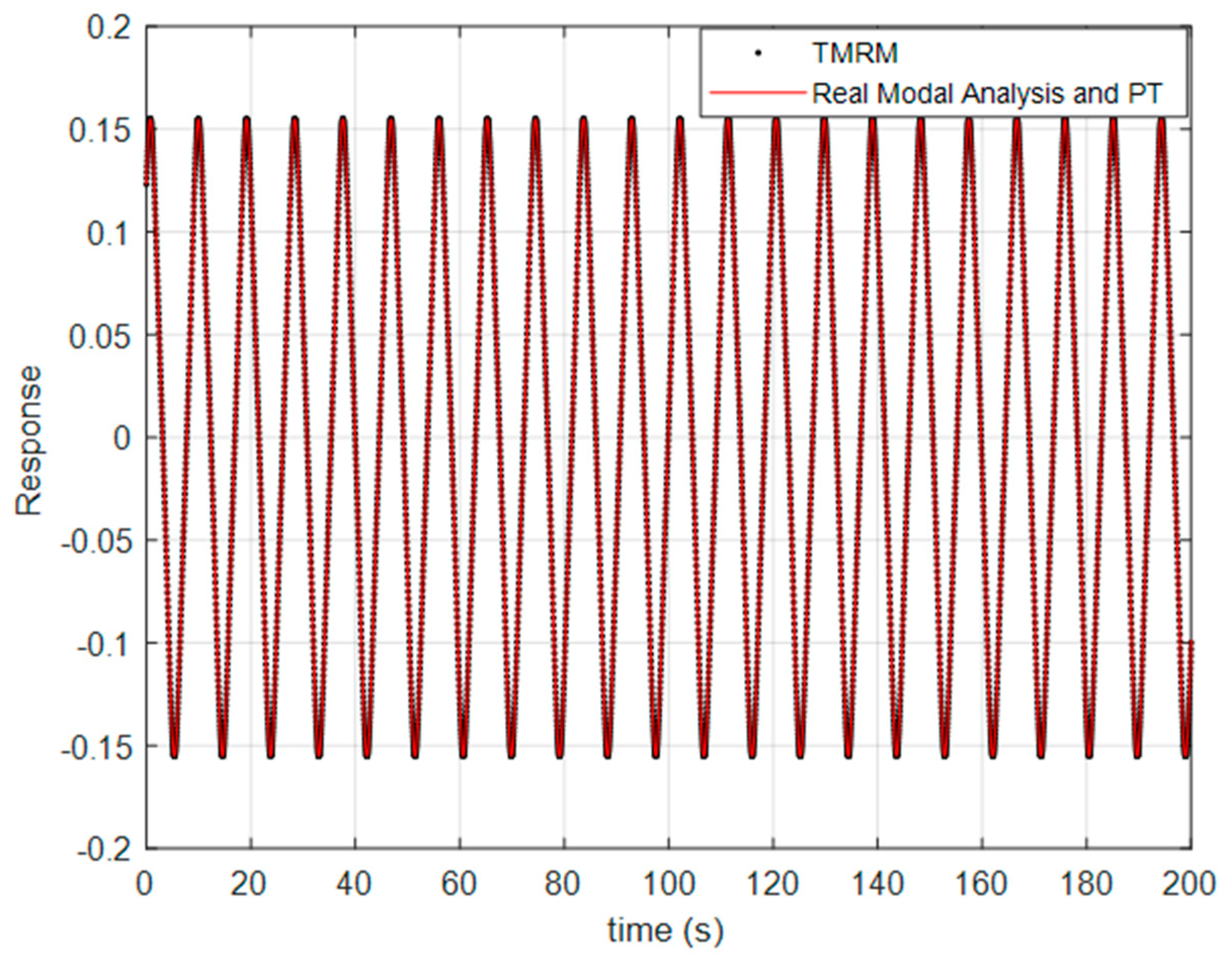
Based on the above recursive relationship, the solution of the system can be obtained. Numerical simulation of the system was conducted and compared with the time-domain minimum residual method (TMRM) calculation results at N = 12 in reference [27], resulting in Figure 1 and

Table 1. Numerical comparison using TMRM and real modal analysis combined with PT method.

t	Modal Analysis with PT3-$\mathit{a}$	TMRM (N = 12)-$\mathit{a}$
20	0.11965	0.11976
40	−0.00120	−0.00116
60	−0.12997	−0.12962
80	−0.11280	−0.11330
100	0.00843	0.00778
120	0.13606	0.13542
140	0.10573	0.10664
160	−0.01553	−0.01448
180	−0.14147	−0.14063
200	−0.09851	−0.09984

of the $a$ curve.

The black dots in Figure 1 represent the $a$ values calculated by the TMRM when N = 12, while the red line shows the $a$ values obtained by combining the real modal analysis with the P-T method. As shown in Figure 1 and Table 1, the displacement-time diagrams calculated by the real modal analysis with the P-T method and those by the TMRM are nearly identical, with minimal numerical differences in the solutions. For ease of analysis,

Table 2. Comparison of computational performance between TMRM and real modal analysis with PT method in terms of CPU time and numerical error.

Method	Modal Analysis with PT3	TMRM (N = 12)
CPU time (s) i5-1335U, CPU 1.3 GHz, RAM 16 GB	3.417807	18.600525
$a$ Maximum relative error	0.0771
$a$ Average relative error	0.0219

provides the computational time and error.

As shown in Table 2, it is evident that the CPU computation time for the real modal analysis combined with the P-T method is shorter than that of the TMRM when N = 12. The average relative error of the solution is less than 3%, with a maximum relative error of less than 10%. This indicates that the time-history response obtained by combining the real modal analysis with the P-T method aligns well with that of the TMRM. The combination of the real modal analysis and the P-T method achieves an ideal balance between efficiency and accuracy. This characteristic of achieving significant performance improvement while ensuring calculation accuracy makes the combination of the real modal analysis and the P-T method have important research value and application potential.

To verify the reliability of the method proposed in this paper, this section first analyzes a benchmark case. In this case, under the condition that the dimensionless flow velocity parameter is equal to 8, the solution obtained by combining real-mode analysis with the PT3 method was quantitatively compared with the semi-analytical solution obtained by the TMRM in reference [27], and the error results are shown in Table 2. The verification of this benchmark case has laid a foundation for the subsequent study of the dynamic characteristics of nonlinear inertial coupling systems with multiple parameters. The subsequent research mainly analyzed the dynamic behavior of the system under different parameters, and the results were verified by comparing the phase diagram with the reports in reference [28] to see if they were consistent.

To explore the dynamic characteristics of the inertially coupled nonlinear vibration system, this paper comprehensively employs methods such as time history diagram, phase diagram, Poincaré mapping, and Periodicity Ratio. Multiple methods corroborate and complement each other, jointly revealing the evolution process of the system from periodic motion to a chaotic state.

Firstly, the time history diagram provides the most intuitive initial judgment. It shows through the displacement variation curve over time how the system motion evolves from a regular periodic waveform to irregular oscillation through period-doubled bifurcation. The phase diagram reveals the global form of the system’s motion through the relationship between displacement and velocity. Its motion curve evolves from the periodic motion of a closed curve to a chaotic motion with complex, disordered, and never-repeating curves. When the system motion is extremely complex, it is easy to misjudge the dynamic behavior merely based on the time history diagram and phase diagram, while the Poincaré mapping provides a decisive objective basis for accurate judgment. It transforms continuous trajectories into discrete point sets. Periodic motion corresponds to a finite number of discrete points; for instance, one point corresponds to period 1 motion, and two points correspond to period 2 motion. Quasi-periodic motion is manifested as a closed curve loop, while chaotic motion is represented as a dense point cloud with a complex structure.

To obtain a quantitative indicator that does not rely on subjectivity, this paper adopts the periodic ratio proposed in reference [23]. This method calculates a value between 0 and 1 through the formula $\gamma =\underset{n\to \infty }{\lim }{\displaystyle \frac{NPP}{n}}$, where $n$ is the total number of all points in the Poincaré mapping and $NPP$ is the number of overlapping points. $\gamma =1$ represents perfect periodic motion, $\gamma =0$ represents complete aperiodic motion, and $0<\gamma <1$ indicates motion that lies between perfect periodic motion and complete aperiodic motion.

Based on the above methods, we conducted an in-depth analysis of the dynamic behavior of the system under different dimensionless flow velocities.

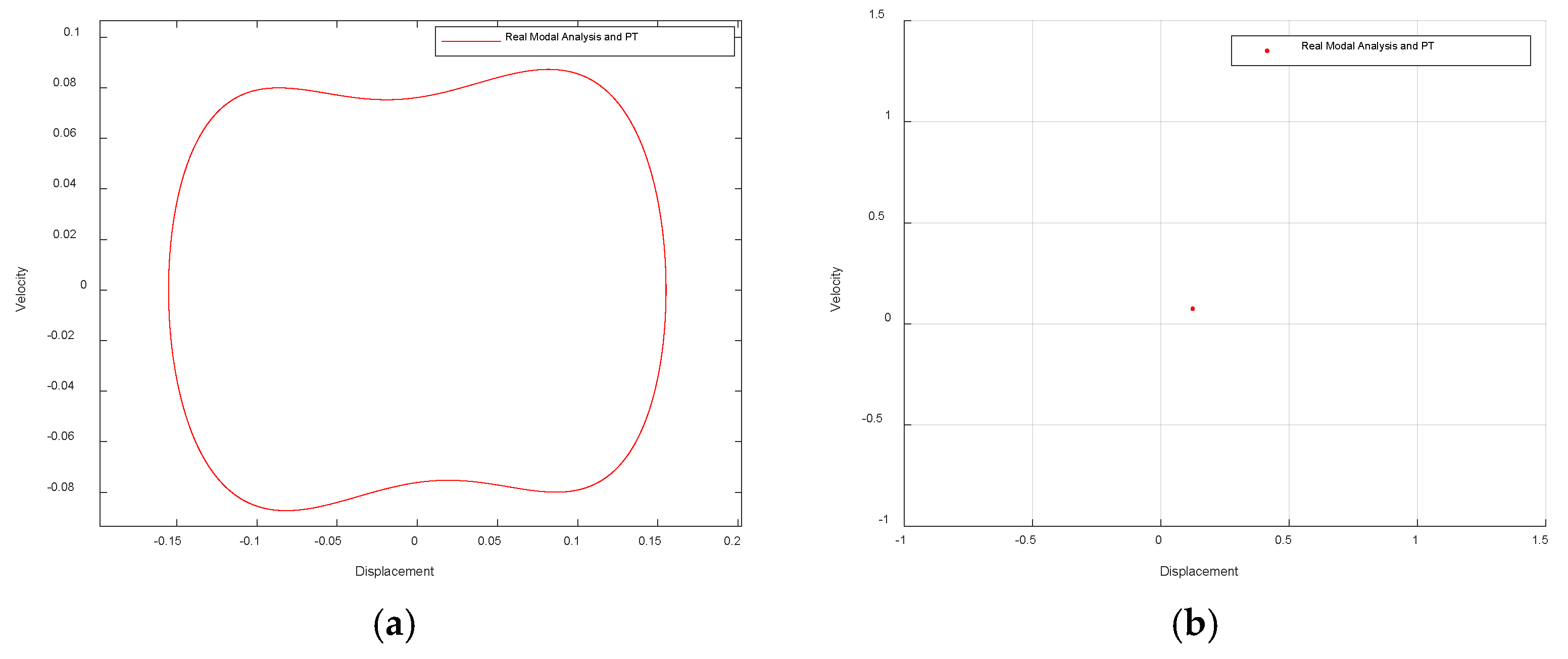
The periodicity ratio of the system is determined to be 1 by the periodicity ratio method [23], so the system is undergoing periodic motion. In Figure 2, (a) shows a phase diagram and (b) shows a Poincaré mapping diagram. The phase diagram is a closed curve. There is a red point in the Poincaré map. Combined with Figure 1, it can be seen that the system moves along a closed curve with a period of 1, and the trajectory has a slight convergence trend.

The periodic motion dynamic behavior of the inertially symmetric coupled nonlinear vibration system has been analyzed in the previous text. However, when the parameters change further, the periodic motion may no longer be stable, and the system may enter a more complex dynamic state. Research shows that, when the periodic solution undergoes an infinite number of multiple periodic bifurcations, the system will eventually enter a chaotic state. The unpredictability of the chaotic state and its sensitivity to the initial conditions will have an impact on the system’s behavior.

To deeply research the dynamic characteristics of the system, this paper combines the theoretical analysis and numerical results of the existing literature and conducts systematic research through methods such as bifurcation diagrams, time history diagrams, phase diagrams, Poincaré mapping diagrams, and periodicity ratios. In the existing research literature, many scholars have constructed inertially symmetric coupled nonlinear vibration systems. Among them, the equations of different motion types established by LC Zhao et al. [28] in their research on analyzing the chaotic behavior of two-dimensional airfoil self-excited force systems are representative. This article will take this system of equations as the entry point to further explore the motion laws of the system. In this paper, the key parameter 0.04 before $Qa$ in the second equation of Equation (24) above is adjusted to 0.07, resulting in the following set of equations:

$$\left\{\begin{array}{ll}{\xi }^{″}+0.25a^{″}+0.1{\xi }^{\prime }+0.2\xi +0.1Qa=0\hfill & \hfill \\ 0.25{\xi }^{″}+0.5a^{″}+0.1a^{\prime }-0.07Qa+0.5a+20a^3=0\hfill & \hfill \end{array}\right.$$

(40)

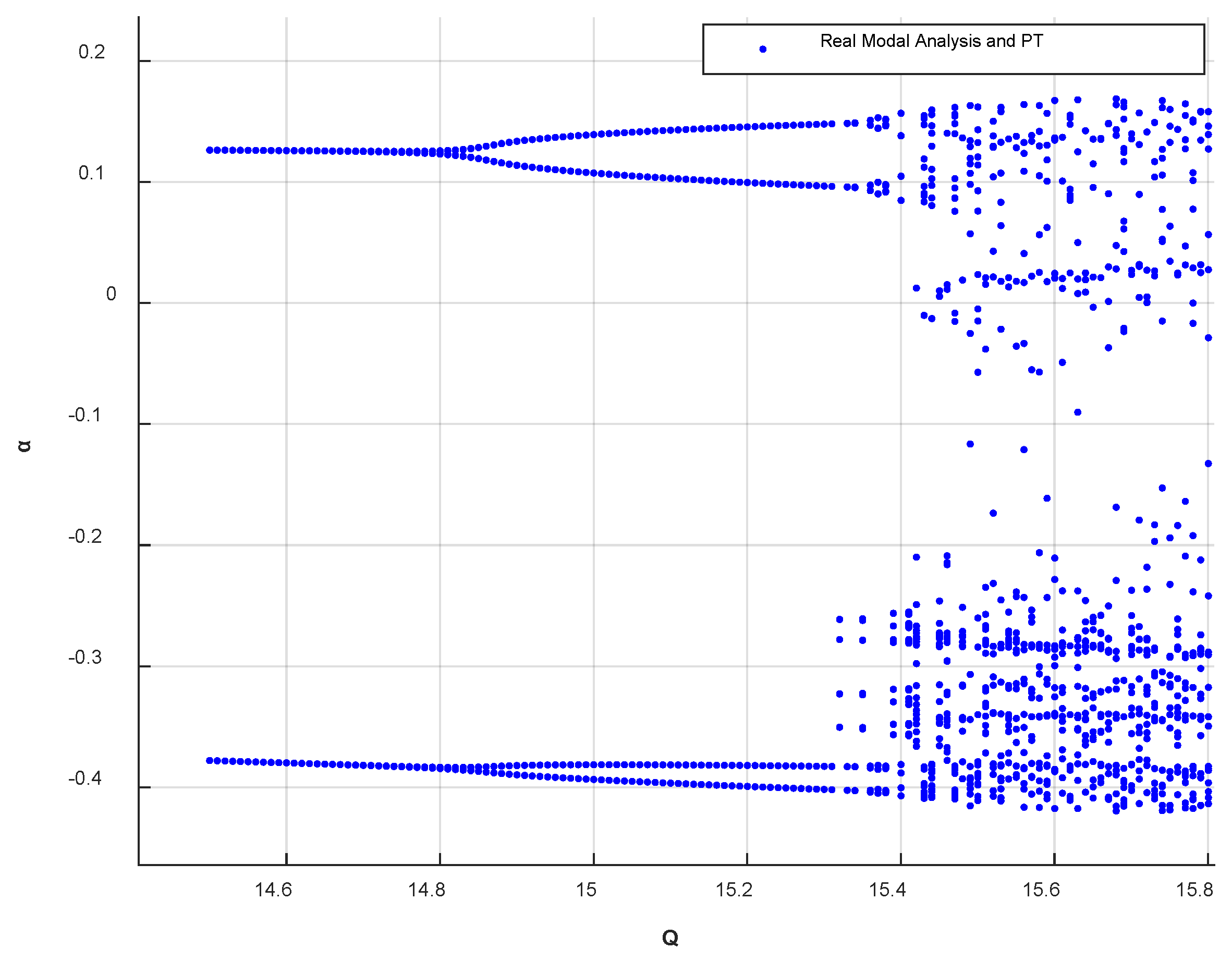
Bifurcation is a core concept for understanding the dynamic behavior of nonlinear systems. It is a phenomenon where the qualitative behavior of the system undergoes a sudden change when the system parameters continuously vary. Because this mutation is very complex, it is difficult to intuitively perceive the characteristics of this dynamic evolution merely through mathematical equations. Bifurcation diagrams, as an important tool for nonlinear system analysis, can obtain the mapping relationship between the visual parameter space and the system state. This paper selects typical bifurcation scenarios of one-period, two-period, four-period, and chaotic motion, and analyzes the corresponding relationship between bifurcation point parameters and the dynamic behavior of the system through the bifurcation diagram (Figure 3).

It can be seen from the bifurcation diagram that there are two points at the beginning of the system, which indicates that there are two different peaks in the system within the same period. At this point, the system is about to bifurcate into a 2-cycle for the first time. Subsequently, a second bifurcation occurs, entering a 4-cycle, after which the bifurcation rate accelerates sharply, quickly entering a chaotic state.

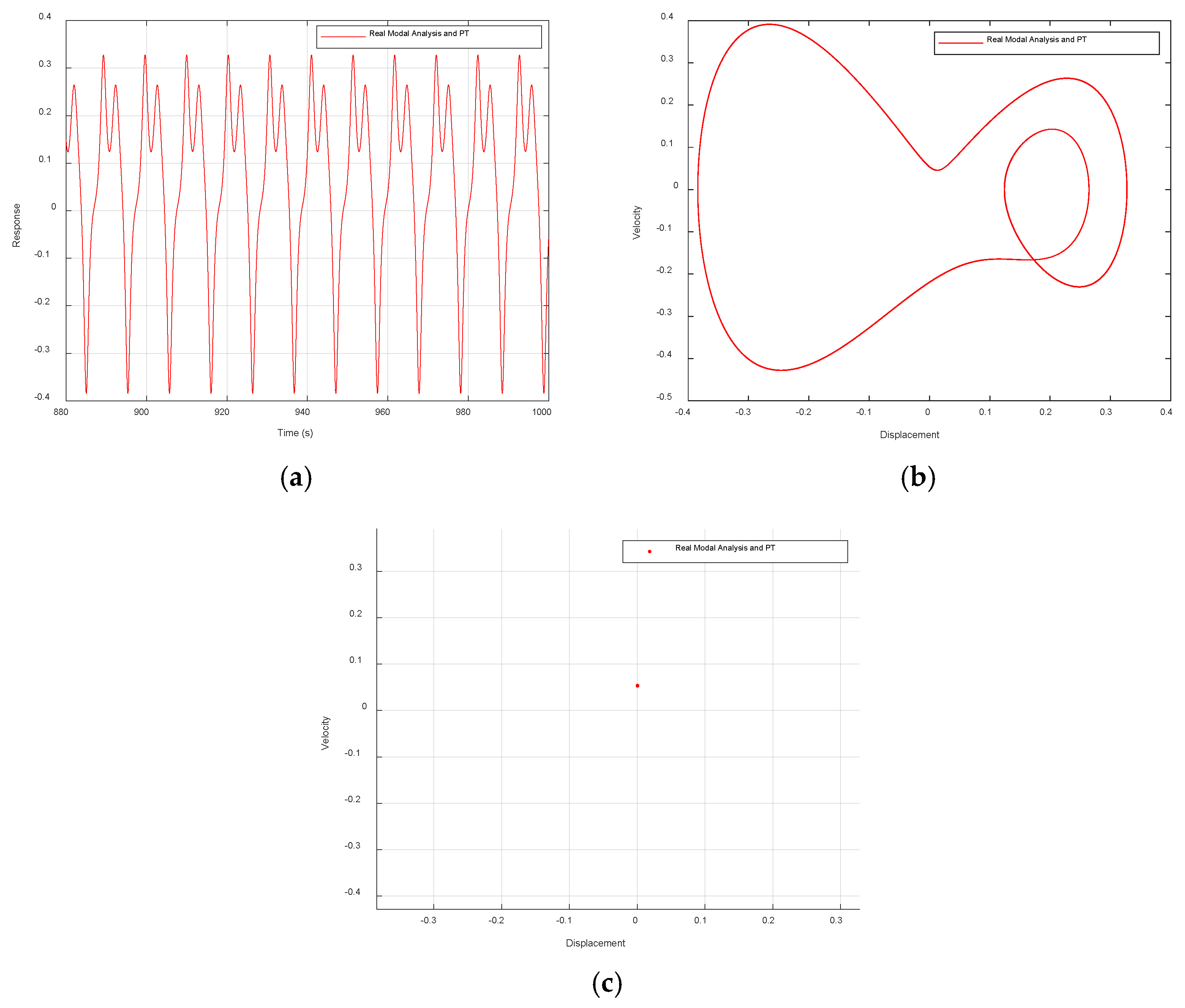
It can be seen from Figure 4 that the system is in a stable periodic motion state. The periodicity ratio of this system is 1. The system repeats the same motion over time with a period of T. The phase diagram is a complex closed-loop curve, and the Poincaré mapping diagram is a point, so this system is in period 1 motion.

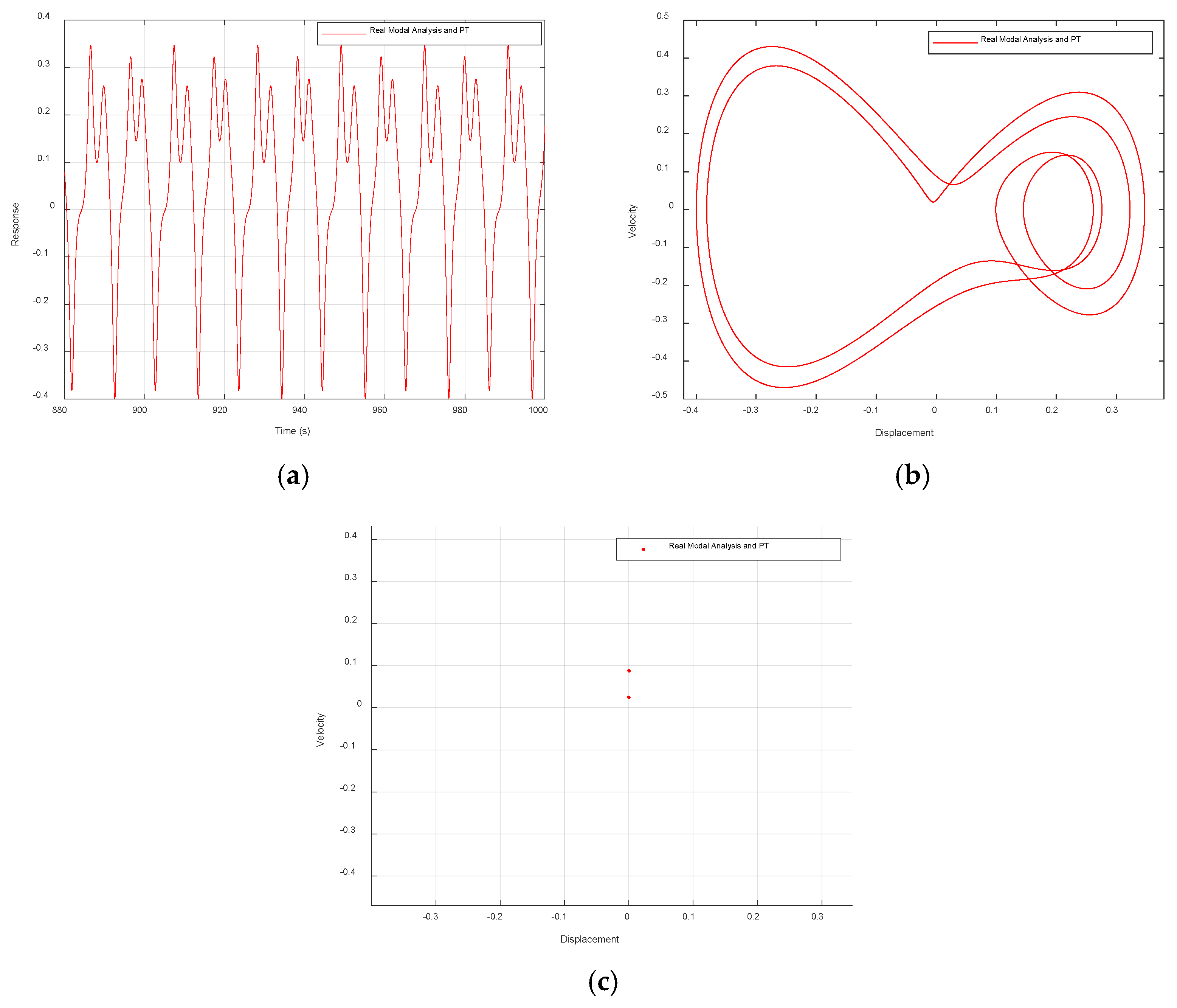
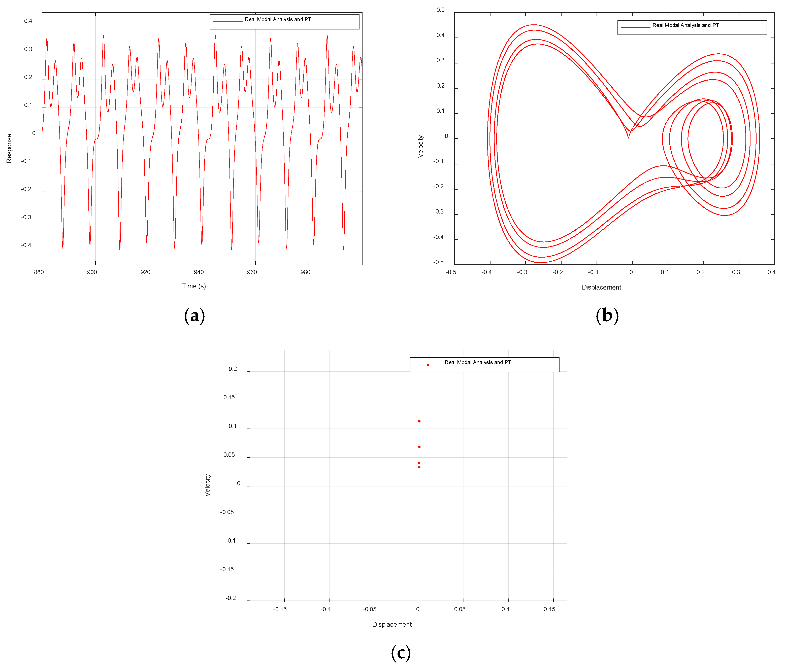
As the dimensionless flow velocity gradually increases, the originally stable periodic motion of period 1 changes, with the original motion becoming unstable and bifurcating into two new stable points. When Q = 15.2, Figure 5 is obtained. The system’s periodicity ratio is 1, and the system’s period doubles to 2T, with the system repeating the motion twice within each period. The phase diagram consists of two closed loop curves, indicating that the system has two distinct periodic motion modes. The Poincaré map consists of two points, so the system exhibits period-2 motion.

As the dimensionless flow velocity increases further, the period-2 motion loses stability again, and the system evolves from period-2 motion to period-4 motion through a double-period bifurcation, which is the path leading to chaos. At that time, $Q=15.4$, resulting in Figure 6. The periodicity ratio of the system is 1, and the period doubles again to 4T. In the time history plot, the waveforms of every four periods are consistent within the error range. The phase diagram consists of four closed loop curves, indicating that the system has four distinct periodic motion modes. The Poincaré map consists of four points, so the system exhibits period-4 motion.

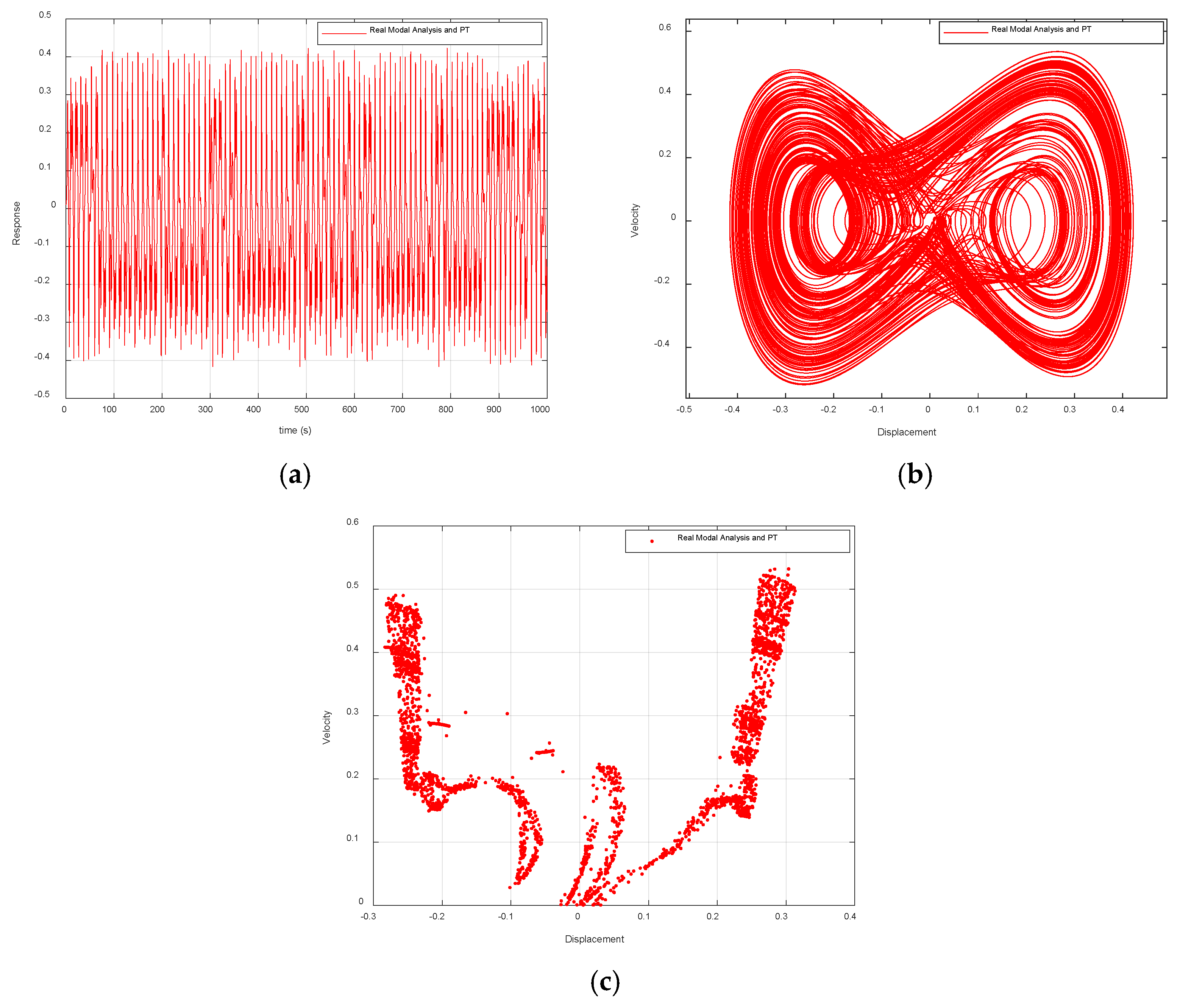
As the dimensionless flow velocity continues to increase, period-doubling infinite bifurcation occurs, eventually transitioning to chaotic motion. When $Q=15.6$, Figure 7 is obtained. The periodicity ratio of this system is 0, and the system undergoes irregular motion over time, with the phase diagram exhibiting a complex and irregular tangled structure. The Poincaré mapping graph changes from four points to a dense point graph with disordered distribution.

Under the condition that the system parameters satisfy Equation (40), the numerical simulation results show that, as the dimensionless flow velocity $Q$ increases, the system eventually enters a chaotic state through period-doubling bifurcation. The time history diagram changes from a regular periodic waveform to an aperiodic oscillation, the phase diagram transforms from a simple closed curve to a complex disordered curve, and the Poincaré mapping changes from a finite number of discrete points to a dense point cloud, clearly presenting the dynamic evolution process towards chaos. This numerical simulation result is in complete agreement with the theoretical analysis conclusion.

3.2. Inertial Asymmetric Coupled Nonlinear Vibration System

The previous text conducted an in-depth analysis of the dynamic behavior of inertially symmetrically coupled nonlinear vibration systems. In this research, based on the assumption of symmetry of the inertia matrix, the system decoupling is achieved through orthogonal transformation, and the solution is obtained by using the real modal analysis combined with the P-T method.

Among the numerical methods for solving coupled nonlinear systems, common ones include the Runge–Kutta method, etc. These methods usually involve step-by-step iterative calculations based on discrete time steps, and the final results are a series of numerical solutions at discrete time points. However, the real modal analysis combined with the P-T method has significant advantages, as it can obtain the continuous solution of the system. This feature is of vital importance because continuous solutions can present the dynamic evolution process of the system over the entire period more completely and accurately.

To verify the feasibility of this method in inertial asymmetric coupled nonlinear systems, this chapter takes the complex dynamic response of binary wings in supersonic flows as the research object. Through the combination of numerical simulation and theoretical analysis, the dynamic behavior of the system is explored.

Here, $\xi$ represents the vertical displacement, $a$ is the pitch Angle, $V$ is the dimensionless flow velocity, and other parameters are taken from reference [20]: $\mu =50$, $x_0=0.5$, $\overline{\omega }=1.0$, $x_a=0.25$, $r_a^2=0.5$, $\alpha =0.5$, ${\zeta }_h={\zeta }_a=0.1$, $\gamma =1.4$, $e=20$, $M_a=6$. The initial condition of this system is $(\xi ,{\xi }^{\prime },a,a^{\prime })=(0,0,0.001,0)$. The dimensionless motion equation of the wing is written as

$$\begin{array}{l}{\xi }^{″}+x_a{a}^{″}+2{\xi }_h{\displaystyle \frac{\overline{\omega }}{V}}{\xi }^{\prime }+{({\displaystyle \frac{\overline{\omega }}{V}})}^2\xi \\ =-{\displaystyle \frac{1}{\mu M_a}}[a+{\xi }^{\prime }+(1-x_0)a^{\prime }+{\displaystyle \frac{1}{12}}{M_a}^2(1+\gamma )a^3]\\ {\displaystyle \frac{x_a}{r_a^2}}{\xi }^{″}+a^{″}+2{\xi }_a{\displaystyle \frac{1}{V}}{a}^{\prime }+{\displaystyle \frac{1}{V^2}}a+{\displaystyle \frac{e}{V^2}}{a}^3\\ ={\displaystyle \frac{1}{\mu M_a{r}_a^2}}[(1-x_0)a+(1-x_0){\xi }^{\prime }+({\displaystyle \frac{4}{3}}-2x_0+{x_0}^2)a^{\prime }+{\displaystyle \frac{1}{12}}{M_a}^2(1-x_0)(1+\gamma )a^3]\end{array}$$

(41)

Substituting the parameters, the dynamic equation is rewritten as

$$\left\{\begin{array}{ll}{\xi }^{″}+0.25a^{″}+({\displaystyle \frac{0.2}{V}}+{\displaystyle \frac{1}{300}}){\xi }^{\prime }+{\displaystyle \frac{1}{600}}{a}^{\prime }+{\displaystyle \frac{1}{V^2}}\xi +{\displaystyle \frac{1}{300}}a+{\displaystyle \frac{3}{125}}{a}^3=0\hfill & \hfill \\ 0.5{\xi }^{″}+a^{″}-{\displaystyle \frac{1}{300}}{\xi }^{\prime }+({\displaystyle \frac{0.2}{V}}-{\displaystyle \frac{7}{1800}})a^{\prime }+({\displaystyle \frac{1}{V^2}}-{\displaystyle \frac{1}{300}})a+({\displaystyle \frac{20}{V^2}}-{\displaystyle \frac{3}{125}})a^3=0\hfill & \hfill \end{array}\right.$$

(42)

The mass matrix in Equation (42) is asymmetric and does not satisfy the premise of real-mode decoupling. The basic conditions for modal decoupling are achieved by converting the sub-diagonal coefficients of the inertia term into the least common multiple.

$$\left\{\begin{array}{ll}2{\xi }^{″}+0.5a^{″}+({\displaystyle \frac{0.4}{V}}+{\displaystyle \frac{1}{150}}){\xi }^{\prime }+{\displaystyle \frac{1}{300}}{a}^{\prime }+{\displaystyle \frac{2}{V^2}}\xi +{\displaystyle \frac{1}{150}}a+{\displaystyle \frac{6}{125}}{a}^3=0\hfill & \hfill \\ 0.5{\xi }^{″}+a^{″}-{\displaystyle \frac{1}{300}}{\xi }^{\prime }+({\displaystyle \frac{0.2}{V}}-{\displaystyle \frac{7}{1800}})a^{\prime }+({\displaystyle \frac{1}{V^2}}-{\displaystyle \frac{1}{300}})a+({\displaystyle \frac{20}{V^2}}-{\displaystyle \frac{3}{125}})a^3=0\hfill & \hfill \end{array}\right.$$

(43)

As described in Section 3.1, construct the proportional damping term.

$$M=\left[\begin{array}{cc}2& 0.5\\ 0.5& 1\end{array}\right],C=\left[\begin{array}{cc}0.0559& 0.0033\\ 0.0033& 0.0207\end{array}\right],K=\left[\begin{array}{cc}0.0381& -0.00115\\ -0.00115& 0.0118\end{array}\right],C=0.0089M+K$$

(44)

Decoupling the left side of the equation using the real modal analysis

$$\left\{\begin{array}{c}{q_1}^{″}+0.035{q_1}^{\prime }+0.0261q_1=0\\ {q_2}^{″}+0.0187{q_2}^{\prime }+0.0098q_2=0\end{array}\right.$$

(45)

Through the modal analysis, the dynamic equation can be rewritten as

$$\left\{\begin{array}{c}\begin{array}{l}{q_1}^{″}+0.035{q_1}^{\prime }+0.0261q_1=\\ ((0.0033-{\displaystyle \frac{1}{300}})g_1{g}_3+(0.0559-{\displaystyle \frac{0.4}{V}}-{\displaystyle \frac{1}{150}}){g_1}^2+(0.0033+{\displaystyle \frac{0.5}{150}})g_1{g}_3+(0.0207-{\displaystyle \frac{0.2}{V}}+{\displaystyle \frac{7}{1800}}){g_3}^2){q_1}^{\prime }\\ +((0.0033-{\displaystyle \frac{1}{300}})g_1{g}_4+(0.0559-{\displaystyle \frac{0.4}{V}}-{\displaystyle \frac{1}{150}})g_1{g}_2+(0.0033+{\displaystyle \frac{0.5}{150}})g_2{g}_3+(0.0207-{\displaystyle \frac{0.2}{V}}+{\displaystyle \frac{7}{1800}})g_4{g}_3){q_2}^{\prime }\\ +((0.0381-{\displaystyle \frac{2}{V^2}}){g_1}^2+(-0.00115-{\displaystyle \frac{1}{150}})g_1{g}_3-0.00115g_1{g}_3+(0.0118-{\displaystyle \frac{1}{V^2}}+{\displaystyle \frac{1}{300}}){g_3}^2)q_1\\ +((0.0381-{\displaystyle \frac{2}{V^2}})g_1{g}_2+(-0.00115-{\displaystyle \frac{1}{150}})g_1{g}_4-0.00115g_2{g}_3+(0.0118-{\displaystyle \frac{1}{V^2}}+{\displaystyle \frac{1}{300}})g_4{g}_3)q_2\\ +(-0.048g_1{g_3}^3-({\displaystyle \frac{20}{V^2}}-{\displaystyle \frac{3}{125}}){g_3}^4){q_1}^3+(-0.048g_1{g_4}^3-k_5{g}_3{g_4}^3){q_2}^3\\ +(-0.144g_1{g_3}^2{g}_4-({\displaystyle \frac{60}{V^2}}-{\displaystyle \frac{9}{125}}){g_3}^3{g}_4){q_1}^2{q}_2+(-0.144g_1{g_4}^2{g}_3-({\displaystyle \frac{60}{V^2}}-{\displaystyle \frac{9}{125}}){g_4}^2{g_3}^2){q_2}^2{q}_1\end{array}\\ \begin{array}{l}{q_2}^{″}+0.0187{q_2}^{\prime }+0.0098q_2=\\ ((0.0033-{\displaystyle \frac{1}{300}})g_2{g}_3+(0.0559-{\displaystyle \frac{0.4}{V}}-{\displaystyle \frac{1}{150}})g_1{g}_2+(0.0033+{\displaystyle \frac{0.5}{150}})g_1{g}_4+(0.0207-{\displaystyle \frac{0.2}{V}}+{\displaystyle \frac{7}{1800}})g_3{g}_4){q_1}^{\prime }\\ +((0.0033-{\displaystyle \frac{1}{300}})g_2{g}_4+(0.0559-{\displaystyle \frac{0.4}{V}}-{\displaystyle \frac{1}{150}}){g_2}^2+(0.0033+{\displaystyle \frac{0.5}{150}})g_2{g}_4+(0.0207-{\displaystyle \frac{0.2}{V}}+{\displaystyle \frac{7}{1800}}){g_4}^2){q_2}^{\prime }\\ +((0.0381-{\displaystyle \frac{2}{V^2}})g_1{g}_2+(-0.00115-{\displaystyle \frac{1}{150}})g_3{g}_2-0.00115g_1{g}_4+(0.0118-{\displaystyle \frac{1}{V^2}}+{\displaystyle \frac{1}{300}})g_3{g}_4)q_1\\ +((0.0381-{\displaystyle \frac{2}{V^2}}){g_2}^2+(-0.00115-{\displaystyle \frac{1}{150}})g_4{g}_2-0.00115g_2{g}_4+(0.0118-{\displaystyle \frac{1}{V^2}}+{\displaystyle \frac{1}{300}}){g_4}^2)q_2\\ +(-0.048g_2{g_3}^3-({\displaystyle \frac{20}{V^2}}-{\displaystyle \frac{3}{125}})g_4{g_3}^3){q_1}^3+(-0.048g_2{g_4}^3-({\displaystyle \frac{20}{V^2}}-{\displaystyle \frac{3}{125}}){g_4}^4){q_2}^3\\ +(-0.144g_2{g_3}^2{g}_4-({\displaystyle \frac{60}{V^2}}-{\displaystyle \frac{9}{125}}){g_3}^2{g_4}^2){q_1}^2{q}_2+(-0.144g_2{g_4}^2{g}_3-({\displaystyle \frac{60}{V^2}}-{\displaystyle \frac{9}{125}}){g_4}^3{g}_3){q_2}^2{q}_1\end{array}\end{array}\right.$$

(46)

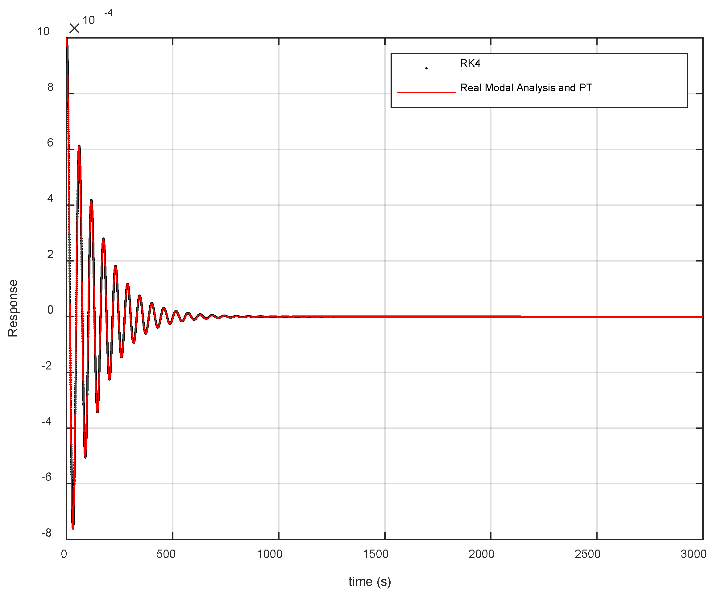
The P-T method, combined with the real modal analysis, was used to perform a numerical simulation of the dynamic response curve $a(t)$ of the system, and the results were compared and analyzed with those obtained using the RK4 method. Using the numerical solution from the RK4 method as the reference, the maximum relative error and average relative error of the P-T method combined with the real modal analysis were quantitatively evaluated, resulting in the comparison curve Figure 8 and error data

Table 3. The solution value at step 0.1 is obtained by RK4 and a 3rd-order PT method combined with real modal analysis method.

t	Modal Analysis with PT3-$\mathit{a}$	RK4-$\mathit{a}$
10	0.000509433	0.000509238
20	−0.000380470	−0.000380450
30	−0.000761593	−0.000760767
40	−0.000348164	−0.000347366
50	0.000348629	0.000347942
60	0.000609284	0.000607412
70	0.000228794	0.000228000
80	−0.000335475	−0.000333785
90	−0.000491342	−0.000488820
100	−0.000127400	−0.000127102

.

In Figure 8, the black dots are the $a$ values obtained by the RK4 method, and the red lines are the $a$ values obtained by the combination of the real modal analysis and the P-T method. Judging from the contents presented in Figure 6 and Table 3, the time history graphs calculated by combining the real modal analysis with the P-T method and the RK4 method show a high degree of consistency and almost complete overlap. For the convenience of subsequent in-depth analysis, the relevant error data are listed in

Table 4. Error of the real modal analysis combined with PT method and RK4 method.

Method	Modal Analysis with PT3	RK4
$a$ Maximum relative error	0.0051594
$a$ Average relative error	0.0024924

.

It can be seen from Table 4 that the maximum and average relative errors of the two methods are very small, indicating that the results obtained by the two solution methods are very close. The results of the real modal analysis combined with the P-T method are reliable and feasible for use in examples. The validity and accuracy of the real modal analysis combined with the P-T method were verified.

In this section, a dimensionless flow velocity parameter equal to 8.132 is selected as the benchmark case. The solution obtained by combining real-mode analysis with the PT3 method is compared with that of the RK4 method in reference [20]. The error results are shown in Table 4. After the method validation, this section further studies the dynamic characteristics of the system under different parameters. The dynamic results of all parameter cases are consistent with the description in reference [20].

To explore the dynamic characteristics of inertial asymmetric coupled nonlinear vibration systems, phase diagrams and Poincaré mapping diagrams are drawn.

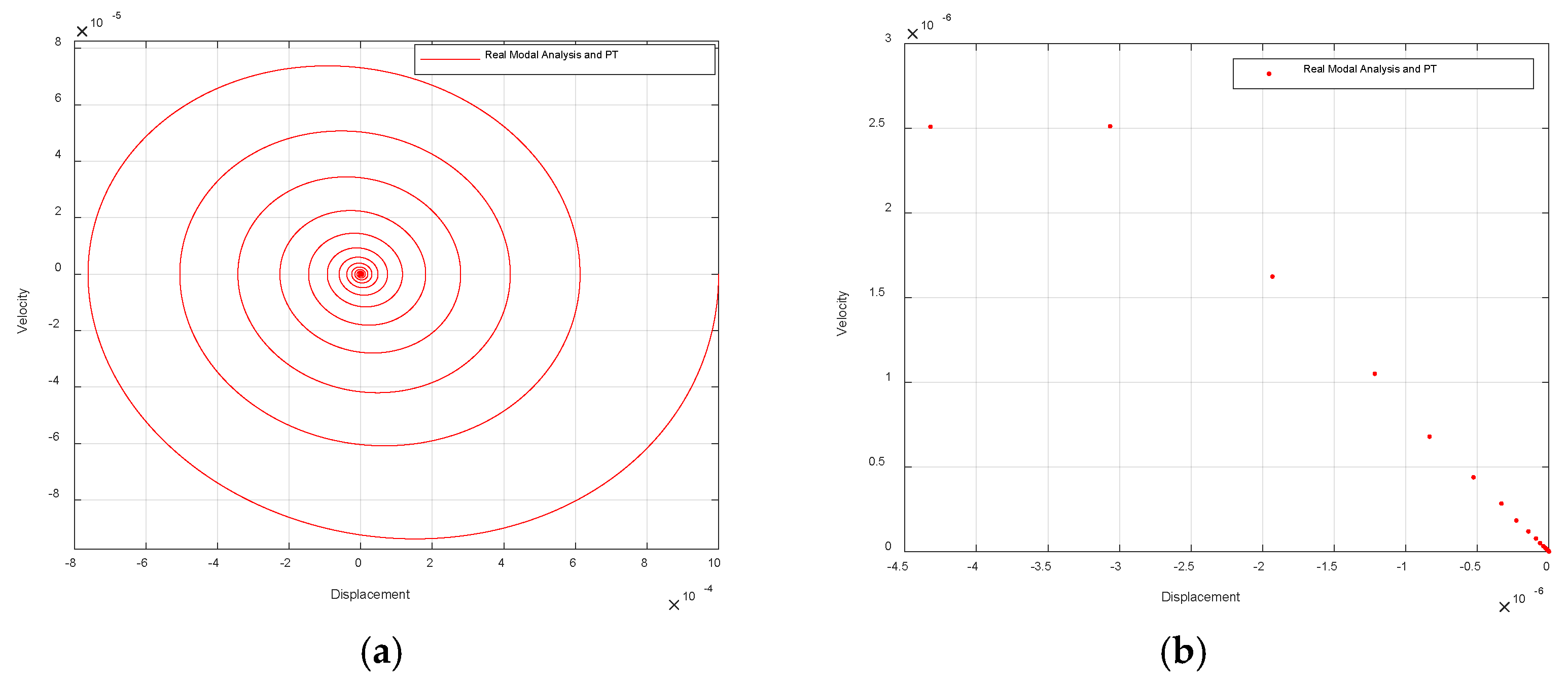
Figure 9 shows that the system exhibits damped oscillation behavior, with the amplitude gradually decreasing over time and eventually approaching a standstill. The Poincaré mapping diagram forms a continuous trajectory that converges inward, intuitively reflecting the evolution process of the system state towards the equilibrium point.

To research the evolution process of the system’s dynamic state, the value of the dimensionless flow velocity V was adjusted based on reference [20] to observe the changes in the system’s behavior. When V gradually increases from 8.132 to 17.934, the system transitions from decaying oscillation to chaotic motion.

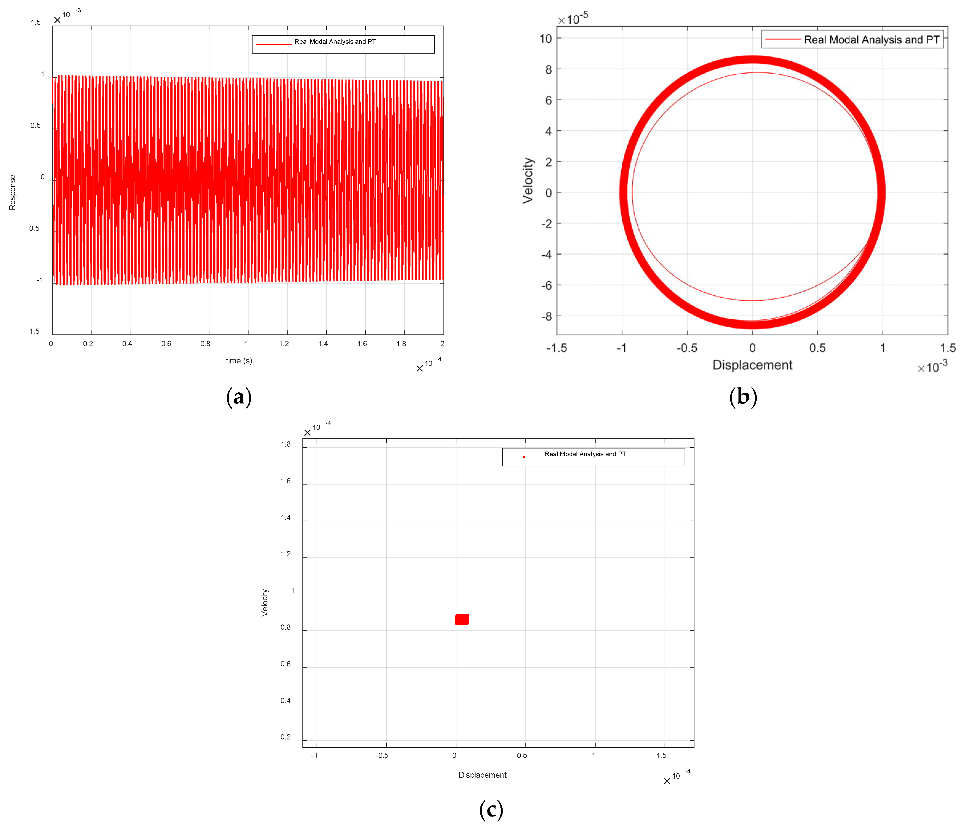
Figure 10 shows that the system exhibits the characteristics of micro-amplitude limit loop oscillation motion. It can be seen from the time history diagram (a) that the response gradually decays to a slight oscillation after periodic motion. The phase diagram (b) is shown as a closed loop, and there is one discrete point in the Poincaré mapping diagram (c). Combined with the periodicity ratio being 1, it can be known that the system tends to the stable limit cycle.

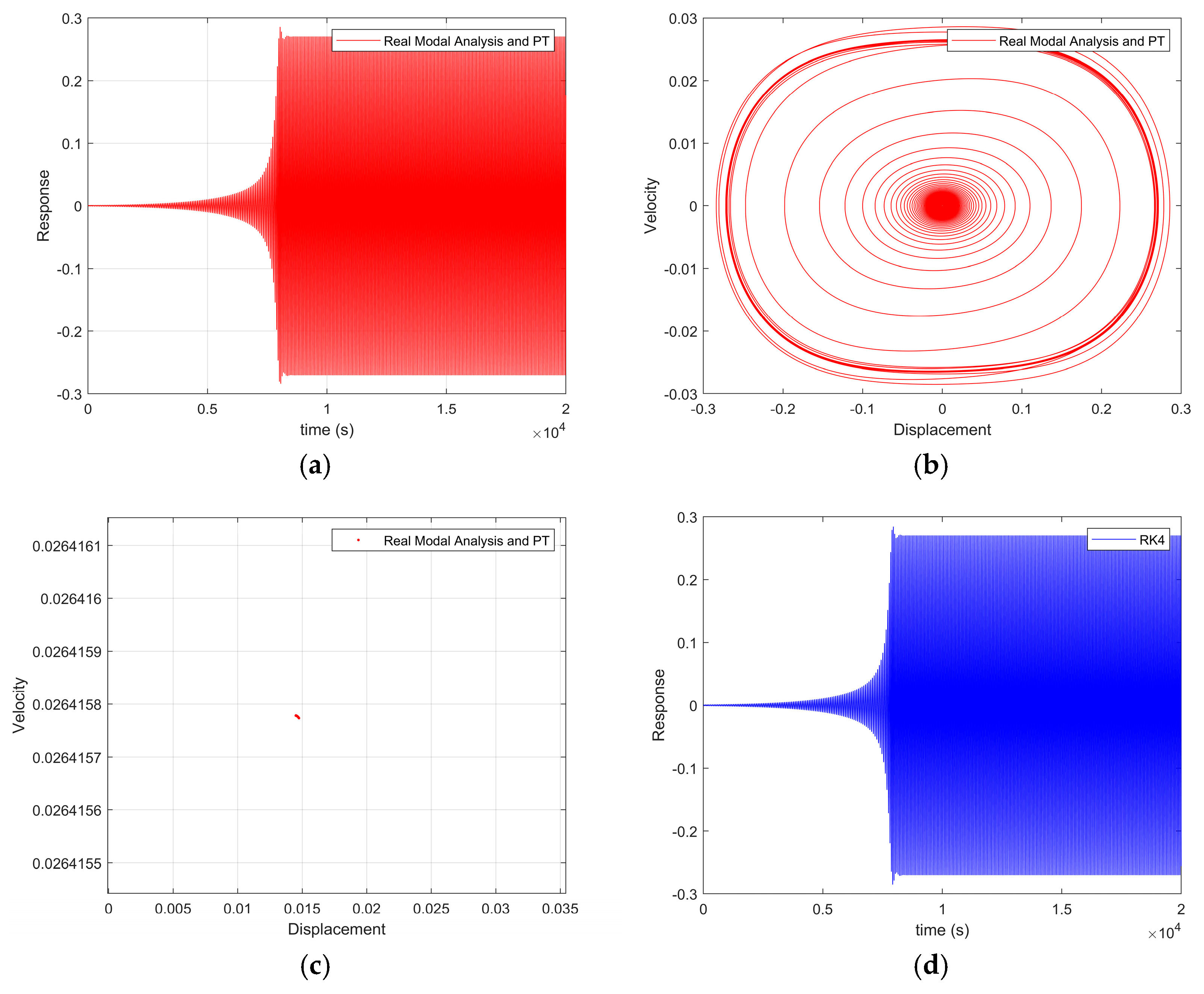
Figure 11 shows that the system initially performs divergent motion. From the moment t = 8038 s, the system’s motion state changes and eventually enters a stable periodic motion. The time history diagram (a) shows that, after the system response diverges, it enters a regular periodic oscillation. In phase diagram (b), when the trajectory expands outward from the center, it corresponds to the divergence stage, and then gradually contracts and eventually converges into a stable closed curve. The Poincaré mapping diagram (c) shows that there is only one mapping point in the stable motion stage. Combined with the periodicity ratio being 1, the system performs a period 1 motion.

The time history diagram (a) in Figure 12 shows the response to irregular fluctuations, the phase diagram (b) shows complex intertwined trajectories, and the Poincaré mapping (c) shows that a large number of non-repetitive trajectory points converge into a structurally complex dense point cloud. It is indicated that the system has chaotic characteristics [29], is sensitive to initial conditions, and its long-term behavior is unpredictable. Combined with a periodicity ratio of 0, the system performs chaotic motion.

This paper reveals the transition path of the system from periodic oscillation to chaotic oscillation by varying the dimensionless flow velocity and combining multiple analytical methods, including time history diagrams, phase portraits, Poincaré maps, and Periodicity Ratio. As shown in Section 3.1, the system undergoes a typical period-doubling bifurcation, where period-1 motion evolves into period-2 motion, then into period-4 motion, and finally leads to chaos. Section 3.2 further demonstrates the dynamic evolution process from convergence, limit cycle oscillation, and periodic motion, to chaos. These results collectively prove that the dimensionless flow velocity is a key control parameter affecting the system’s transition from regular motion to chaotic motion.

To verify the reliability of the theoretical analysis results, by graphically comparing the calculation results of the real modal analysis combined with the P-T method with the literature, it was found that panel (c) of Figure 1 in the literature [20] misjudged the motion of the system as divergent motion due to insufficient simulation time (t = 3000 s). This research found that by extending the simulation time to t = 20,000 s, the system exhibited periodic motion (Figure 11). To exclude methodological specificity, we adopted RK4 for verification under the same duration, as shown in Figure 11d. The results indicate the system ultimately stabilizes, completely consistent with the results obtained by this paper’s real modal analysis combined with the P-T method. This correction reveals the limitations of short-term numerical simulation in nonlinear systems and emphasizes that fully extending the observation time plays a decisive role in accurately identifying the steady-state behavior of the system.

Except for the revised Figure 11, all the other figures show good consistency. This comparison result not only fully verifies the computational accuracy of the real modal analysis combined with the P-T method in solving the dynamic response problems of such nonlinear systems, but also further supports the aforementioned theoretical analysis conclusion on the evolution of the system with dimensionless flow velocity.

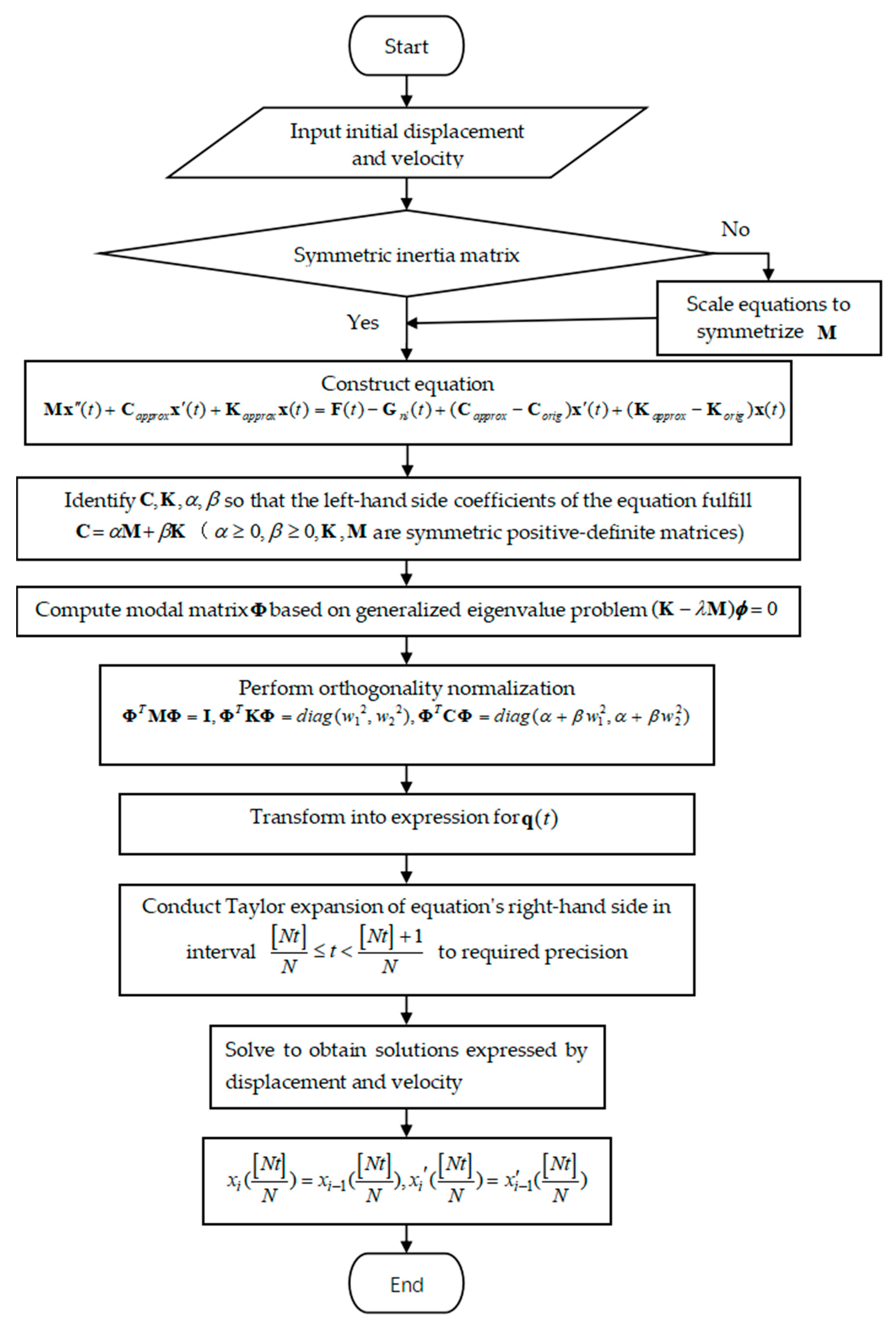
To facilitate the understanding of the specific process of the combination of Real Modal Analysis and the P-T method, Figure 13 provides the following flowchart for elaboration.

4. Conclusions

This paper employs the real modal analysis, combined with the P-T method, to derive a semi-analytical solution for inertially coupled nonlinear systems. It verifies the effectiveness of the method using a two-dimensional wing flutter model. Finally, the dynamic behavior is analyzed using time history diagrams, phase diagrams, Poincaré maps, and periodicity ratios. The following conclusions are drawn:

• The TMRM and real modal analysis combined with the P-T method are both semi-analytical methods. In the case described in Section 2.1, the comparison results of the solution of the real modal analysis combined with the third-order P-T method and the solution of the TMRM at N = 12 show that the average relative error is less than 3% and the maximum relative error is less than 10%, indicating that the results of the two methods have good consistency. More importantly, in terms of computational efficiency, real modal analysis combined with the P-T method shows significant advantages. Its CPU computing time is reduced by approximately 15.18 s compared to TMRM (N = 12).
• When using the RK4 method to solve the inertial coupled system, the second-order differential equation needs to be reduced to a first-order system of equations, thereby obtaining discrete numerical solutions. This order reduction process alters the mathematical formal structure of the original system, which may lead to the loss of its mathematical features. In this paper, by using the strategy of real modal analysis combined with the P-T method, the solution is always carried out within the framework of the second-order system, which not only maintains the consistency of the mathematical form but also makes full use of the mathematical characteristics of the system. For example, based on the symmetry of matrices and the structure of second-order differentiation, decoupling is achieved through linear algebraic methods such as generalized eigenvalue decomposition and orthogonal transformation, and then solved by the P-T method to obtain a continuous semi-analytical solution.
• This paper reveals the complex and diverse motion patterns of nonlinear systems through period-doubling bifurcation and order-to-chaos transitions. The dimensionless flow velocity is a key control parameter that influences the state changes of the system. Therefore, precise control of the dimensionless flow velocity to avoid wing divergence and chaotic motion is crucial for ensuring the flight safety of aircraft.
• This paper adopts a solution strategy that combines real-mode analysis with the P-T method. First, through mathematical preprocessing methods, each equation of the original system of equations is multiplied by a specific scaling factor, respectively, converting the asymmetric second-order term coefficient matrix into a symmetric form. Subsequently, through the moving of terms, the left-hand side of the equation is made to satisfy the proportional damping form $C=\alpha M+\beta K$, while the right side contains linear and nonlinear terms that do not satisfy the proportional damping mathematical form. Then, the mathematical process of real modal analysis is borrowed for decoupling, and it is solved by using the P-T method. Through mathematical means, the application scope of the mathematical framework for real modal analysis has been expanded, enabling it to effectively handle mathematical models where the second-order term coefficient matrix is asymmetric and the damping term does not satisfy the proportional relationship, providing a new idea for the numerical solution of such systems. Future work will explore the application of this method in inertially coupled nonlinear vibration systems with nonlinear inertial terms and attempt to further enhance efficiency.

References

1. Dubatovskaya, M.V.; Rogozin, S.V. Homogeneous characteristic equation with an infinite index in the exceptional case. Dokl. Akad. Nauk. Belarusi 1996, 4, 53–56. [Google Scholar]
2. Moridis, G.J.; Reddell, D.L. The laplace transform finite difference method for simulation of flow through porous media. Water Resour. Res. 1991, 27, 1873–1884. [Google Scholar] [CrossRef]
3. Kabe, A.M.; Sako, B.H. Multi-degree-of-freedom systems. In Structural Dynamics Fundamentals and Advanced Applications; Elsevier: Amsterdam, The Netherlands, 2020; pp. 333–435. [Google Scholar]
4. Jin, D. Method of Polynomial Vectors for Solving Nonlinear Vibrations with Multiple Time Scales. J. Vib. Eng. Technol. 2024, 12, 8179–8187. [Google Scholar] [CrossRef]
5. Aftabizadeh, A.R.; Wiener, J. Oscillatory properties of first order linear functional differential equations. Appl. Anal. 1985, 20, 165–187. [Google Scholar] [CrossRef]
6. Thomaser, A.; De Nobel, J.; Vermetten, D.; Ye, F.; Bäck, T.; Kononova, A. When to be Discrete: Analyzing Algorithm Performance on Discretized Continuous Problems. In Proceedings of the Genetic and Evolutionary Computation Conference, Lisbon, Portugal, 15–19 July 2023. [Google Scholar]
7. Arora, G.; Joshi, V.; Garki, I.S. Developments in Runge–Kutta Method to Solve Ordinary Differential Equations. In Recent Advances in Mathematics for Engineering; CRC Press: Boca Raton, FL, USA, 2020; pp. 193–202. [Google Scholar]
8. Cooke, K.L.; Wiener, J. Stability regions for linear equations with piecewise continuous delay. Comput. Math. Appl. 1986, 12, 695–701. [Google Scholar] [CrossRef]
9. Jayasree, K.N.; Deo, S.G. On piecewise constant delay differential equations. J. Math. Anal. Appl. 1992, 169, 55–69. [Google Scholar] [CrossRef]
10. Dai, L.; Singh, M.C. An analytical and numerical method for solving linear and nonlinear vibration problems. Int. J. Solids Struct. 1997, 34, 2709–2731. [Google Scholar] [CrossRef]
11. Dai, L. Assessment of Solutions to Vibration Problems Involving Piecewise Constant Exertions. In Proceedings of the ASME International Mechanical Engineering Congress and Exposition, Orlando, FL, USA, 5–10 November 2000; pp. 69–72. [Google Scholar]
12. Baum, H.R. On the weakly damped harmonic oscillator. Q. Appl. Math. 1972, 29, 573–576. [Google Scholar] [CrossRef]
13. Big-Alabo, A. Continuous piecewise linearization method for approximate periodic solution of the relativistic oscillator. Int. J. Mech. Eng. Educ. 2018, 48, 178–194. [Google Scholar] [CrossRef]
14. Dahlquist, G.; Bjorck, A. Numerical Methods; Prentice-Hall, Inc.: New Jersey, NJ, USA, 1974. [Google Scholar]
15. Glushchenko, A.I.; Petrov, V.A.; Lastochkin, K.A. DREM procedure application for piecewise constant parameters identification. Sci. Tech. J. Inf. Technol. Mech. Opt. 2021, 134, 449–456. [Google Scholar] [CrossRef]
16. Gerald, C.F.; Wheatley, P.O. Applied Numerical Analysis; Addison-Wesley Publishing Company: New York, NY, USA, 1989. [Google Scholar]
17. Dai, L.; Singh, M.C. A new approach with piecewise-constant arguments to approximate and numerical solutions of oscillatory problems. J. Sound Vib. 2003, 263, 535–548. [Google Scholar] [CrossRef]
18. Dai, L.; Wang, X. Accuracy and Reliability of P-T Method in Studying the Responses of Nonlinear Dynamic Systems. J. Comput. Nonlinear Dynam. 2014, 10, 021009. [Google Scholar] [CrossRef]
19. Fang, P.; Dai, L.; Hou, Y.; Du, M.; Wang, L.; Xi, Z. Numerical Computation for the Inertial Coupling Vibration System Using PL Method. J. Vib. Eng. Technol. 2019, 7, 139–148. [Google Scholar] [CrossRef]
20. Wang, Y.; Zhang, Q.; Zhu, L. Active control of hypersonic airfoil flutter via adaptive fuzzy sliding mode method. J. Vib. Control 2015, 21, 134–141. [Google Scholar] [CrossRef]
21. He, D.; Huang, W.; Wang, Q. Limit cycle flutter and chaotic motion of two-dimensional airfoil system. J. Guangxi Norm. Univ. Nat. Sci. Ed. 2019, 37, 87–95. [Google Scholar]
22. Portegies Zwart, S.F.; Boekholt, T.C.N. Numerical verification of the microscopic time reversibility of Newton’s equations of motion: Fighting exponential Divergence. Commun. Nonlinear Sci. Numer. Simul. 2018, 61, 160–166. [Google Scholar] [CrossRef]
23. Dai, L.; Han, L. Characteristics Diagnosis of Nonlinear Dynamical Systems; Springer: New York, NY, USA, 2012. [Google Scholar]
24. Hagedorn, P.; DasGupta, A. Vibrations and Waves in Continuous Mechanical Systems; Wiley: Hoboken, NJ, USA, 2007. [Google Scholar]
25. Liu, G.; Zhang, M. Orthogonality of Modes and Its Diagonalization Function. J. Chang. Norm. Univ. 2015, 34, 5–7. [Google Scholar]
26. Chen, Y.M.; Liu, J.K. Homotopy analysis method for limit cycle flutter of airfoils. Appl. Math. Comput. 2008, 203, 854–863. [Google Scholar] [CrossRef]
27. Liu, G.; Lu, Z.R.; Wang, L.; Liu, J.K. A new semi-analytical technique for nonlinear systems based on response sensitivity analysis. Nonlinear Dyn. 2021, 103, 1529–1551. [Google Scholar] [CrossRef]
28. Zhao, L.C.; Yang, Z.C. Chaotic motions of an airfoil with non-linear stiffness in incompressible flow. J. Sound Vib. 1990, 138, 245–254. [Google Scholar] [CrossRef]
29. Kong, L.; Liu, D.; Jian, K. Study on chaotic characteristics of heterogeneous physical double pendulum. Chongqing Univ. J. 2024, 47, 106–118. [Google Scholar]
Figure 1. Comparison of time history diagrams obtained by combining TMRM and real modal analysis combined with PT method for Equation (25). ( ξ 0 = 0.3422 , ξ 0 = 0.0663559 , a 0 = 0.1233 , a 0 = 0.0753726 ).
Mathematics 13 03278 g001
Figure 2. Dynamic characteristics of the system at Q = 8 : (a) Phase diagram; (b) Poincaré map.
Mathematics 13 03278 g002
Figure 3. Bifurcation diagram obtained by combining real modal analysis with PT method. ( ξ 0 = 0 , ξ 0 = 0 , a 0 = 0.01 , a 0 = 0 ).
Mathematics 13 03278 g003
Figure 4. Dynamic characteristics of the system at Q = 14.8 : (a) Time history diagram; (b) Phase diagram; (c) Poincaré map.
Mathematics 13 03278 g004
Figure 5. Dynamic characteristics of the system at Q = 15.2 : (a) Time history diagram; (b) Phase diagram; (c) Poincaré map.
Mathematics 13 03278 g005
Figure 6. Dynamic characteristics of the system at Q = 15.4 : (a) Time history diagram; (b) Phase diagram; (c) Poincaré map.
Mathematics 13 03278 g006
Figure 7. Dynamic characteristics of the system at Q = 15.6 : (a) Time history diagram; (b) Phase diagram; (c) Poincaré map.
Mathematics 13 03278 g007
Figure 8. Time history graph obtained by RK4 method and real modal analysis method combined with PT method when V is 8.132. ( ξ 0 = 0 , ξ 0 = 0 , a 0 = 0.001 , a 0 = 0 ).
Mathematics 13 03278 g008
Figure 9. Dynamic characteristics of the system at V = 8.132: (a) Phase diagram; (b) Poincaré map.
Mathematics 13 03278 g009
Figure 10. Dynamic characteristics of the system at V = 10.388: (a) Time history diagram; (b) Phase diagram; (c) Poincaré map.
Mathematics 13 03278 g010
Figure 11. Dynamic characteristics of the system at V = 10.572 : (a) Time history diagram (Real-modal-analysis-based P-T); (b) Phase diagram; (c) Poincaré map; (d) Time history diagram (RK4).
Mathematics 13 03278 g011
Figure 12. Dynamic characteristics of the system at V = 17.934 : (a) Time history diagram; (b) Phase diagram; (c) Poincaré map.
Mathematics 13 03278 g012
Figure 13. Flowchart of real modal analysis combined with P-T method.
Mathematics 13 03278 g013