D-Finite Discrete Generating Series and Their Sections

Abstract

This paper investigates D-finite discrete generating series and their sections. The concept of D-finiteness is extended to multidimensional discrete generating series and its equivalence to p-recursive sequences is rigorously established. It is further shown that sections of the D-finite series preserve D-finiteness, and that their generating functions satisfy systems of linear difference equations with polynomial coefficients. In the two-dimensional case, explicit difference relations are derived that connect section values with boundary data, while in higher dimensions general constructive methods are developed for obtaining such relations, including cases with variable coefficients. Several worked examples illustrate how the theory applies to solving difference equations and analyzing multidimensional recurrent sequences. The results provide a unified framework linking generating functions and recurrence relations, with applications in combinatorics, number theory, symbolic summation, and the theory of discrete recursive filters in signal processing.

1. Introduction and Notation

We consider D-finite discrete generating series because they provide a natural framework for linking multidimensional recurrence relations with generating functions. Unlike the classical power series case, the discrete setting remains less developed, despite its importance in combinatorial enumeration, symbolic summation, and the analysis of difference equations. Studying their sections is particularly relevant, as it shows how structural properties are preserved under variable reduction, with applications ranging from lattice path problems to number theory and discrete recursive filters in signal processing.

The theory of D-finite generating functions in the single-variable case was introduced in [1], and its extension to the multivariate case was developed in [2]. The concept of D-finiteness discussed in [2] refers to a finite-dimensional vector space of solutions to some linear equations. D-finite series supported in rational cones were studied in [3]. A corresponding theory for discrete generating functions was proposed in the one-dimensional case in [4] and extended to the multidimensional setting in [5].

This paper develops a unified framework for analyzing sections of D-finite discrete generating series, highlighting their recurrence properties and applications in combinatorics, symbolic summation, and digital filter design. We derive explicit difference equations for multidimensional generating series, thereby extending existing results on p-recursive sequences and their relationship to generating functions.

Let $f:{\mathbb{Z}}^n\to \mathbb{C}$, $\xi =({\xi }_1,\dots ,{\xi }_n)\in {\mathbb{C}}^n$, and $\ell =({\ell }_1,\dots ,{\ell }_n)\in {\mathbb{Z}}_{⩾}^n$. For a nonnegative integer k and $z\in \mathbb{C}$, we define the falling factorial as

$$z^{\underline{k}}=z(z-1)\dots (z-k+1),z^{\underline{0}}=1$$

and consider discrete generating functions of n variables:

$$\begin{array}{c}F({\xi }_1,\dots ,{\xi }_n;{\ell }_1,\dots ,{\ell }_n;z_1,\dots ,z_n)={\displaystyle \sum _{x_1=0}^{\infty }}\dots {\displaystyle \sum _{x_n=0}^{\infty }}f(x_1,\dots ,x_n){\xi }_1^{x_1}\cdots {\xi }_n^{x_n}{z}_1^{\underline{{\ell }_1{x}_1}}\cdots z_n^{\underline{{\ell }_n{x}_n}},\end{array}$$

or, in a compact multidimensional notation:

$$\begin{array}{c}F(\xi ,\ell ;z)={\displaystyle \sum _{x\in {\mathbb{Z}}_{⩾}^n}}f\left(x\right){\xi }^x{z}^{\underline{\ell x}}.\end{array}$$

Notably, these functions can be regarded as multidimensional analogs of discrete hypergeometric functions, which have been studied in connection with the generalized hypergeometric difference equation [6], the Bessel difference equation [7], and are also of interest in the theory of dynamic equations on time scales [8].

Let $e^j=(0,\dots ,1,\dots ,0)$ be the unit vector with its j-th coordinate equal to one, for $j=1,\dots ,n$. Consider the right difference operator ${\Delta }_{j}f\left(z\right)=f(z+e^j)-f\left(z\right)$ for $j=1,\dots ,n$. Then,

$${\Delta }_j{z}^{\underline{x}}=x_j{z}^{\underline{x-e^j}}.$$

Thus, the operator ${\Delta }_j$ serves as a discrete analog of differentiation, yielding:

$${\Delta }_{j}F(\xi ,\ell ;z)={\Delta }_j\sum _{x⩾0}f\left(x\right){\xi }^x{z}^{\underline{\ell x}}=\sum _{x⩾0}{\ell }_j{x}_{j}f\left(x\right){\xi }^x{z}^{\underline{\ell x-e^j}}.$$

Denote the left shift operator as ${\rho }_{j}F\left(z\right)=F(z-e^j)$ and define

$$x^k=x_1^{k_1}\dots x_n^{k_n}.$$

We then introduce the operators

$${\theta }_j={\ell }_j^{-1}{z}_j{\rho }_j{\Delta }_j,j=1,\dots ,n,$$

$${\theta }^k={\theta }_1^{k_1}\dots {\theta }_n^{k_n},$$

and

$$p\left(\theta \right)=\sum _{\alpha \in A}{c}_{\alpha }{\theta }^{\alpha },$$

where $A\subset {\mathbb{Z}}_{⩾}^n$ is a finite set of points, and $c_{\alpha }\in \mathbb{C}$.

Some useful properties of these operators, proven in [5], include

$$\begin{array}{c}{\theta }^{k}F(\xi ,\ell ;z)={\displaystyle \sum _{x=0}^{\infty }}{x}^{k}f\left(x\right){\xi }^x{z}^{\underline{\ell x}},\\ p\left(\theta \right)F(\xi ,\ell ;z)={\displaystyle \sum _{x=0}^{\infty }}p\left(x\right)f\left(x\right){\xi }^x{z}^{\underline{\ell x}}.\end{array}$$

Now we prove a simple lemma.

Lemma 1.

The following relation holds for all $x=1,2,3,\dots$ and $j=1,\dots ,n$:

$$({\theta }_j-x_j)z^{\underline{\ell x}}=0.$$

Proof. 

Using the definition of ${\theta }_j$, compute

$$({\theta }_j-x_j)z^{\underline{\ell x}}={\theta }_j{z}^{\underline{\ell x}}-x_j{z}^{\underline{\ell x}}=x_j{z}^{\underline{\ell x}}-x_j{z}^{\underline{\ell x}}=0,$$

which completes the proof. □

2. D-Finite Discrete Generating Functions

Let $p_{\alpha }\left(x\right),\alpha =0,\dots ,r$ be polynomials in a single variable x, where $p_r\left(x\right)$ is not identically zero. In [1], sequences $f:\mathbb{Z},\to \mathbb{C}$ that satisfy the recurrence relation

$$\begin{array}{c}{\displaystyle \sum _{\alpha =0}^r}{p}_{\alpha }\left(x\right)f(x+\alpha )=0,\end{array}$$

are called polynomially recursive (p-recursive). In the same work, the concept of differentially finite (D-finite) power series is introduced: a generating series

$$\begin{array}{c}F\left(z\right)={\displaystyle \sum _{x=0}^{\infty }}f\left(x\right)z^x\end{array}$$

is called differentially finite if there exists a set of polynomials $P_0\left(z\right)$, $P_1\left(z\right),\dots$, $P_k\left(z\right)$, and $P\left(z\right)$, at least one of which is not identically zero, such that

$$\begin{array}{c}{\displaystyle \sum _{i=0}^k}{P}_i\left(z\right){\displaystyle \frac{{\mathrm{d}}^i}{\mathrm{d}{z}^i}}F\left(z\right)=P\left(z\right).\end{array}$$

Without loss of generality, we can assume the right-hand side is zero (by differentiating both sides a sufficient number of times).

It should be noted that p-recursive sequences appear in wavelet theory, in a broad class of combinatorial enumeration problems [1,9], and the special cases with constant coefficients has been studied in detail in [10,11,12]. Equations with variable coefficients for lattice paths are considered in [13].

We extend the concepts of p-recursiveness and D-finiteness to the multidimensional case [2]. For $x,y\in {\mathbb{Z}}_{⩾}^n$, the inequality $x⩾y$ means that $x_j⩾y_j$ for all $j=1,\dots ,n$, while the notation $x\ngeqq y$ indicates that $x\in {\mathbb{Z}}_{⩾}^n\setminus (y+{\mathbb{Z}}_{⩾}^n)$ (see Figure 1).

Definition 1.

Let $m,\alpha \in {\mathbb{Z}}_{⩾}^n$, $0⩽\alpha ⩽m$, and let $p_{\alpha ,j}\left(x_j\right)$ be polynomials in a single variable $x_j,j=1,\dots ,n$, not all identically zero. A multidimensional sequence $f\left(x\right):{\mathbb{Z}}^n\to \mathbb{C}$ is called p-recursive if it satisfies the following system:

$$\begin{array}{c}{\displaystyle \sum _{0⩽\alpha ⩽m}}{p}_{\alpha ,j}\left(x_j\right)f(x+\alpha )=0,j=1,\dots ,n,\end{array}$$

(1)

for all $x⩾m$, and all subsequences obtained from $f(x_1,\dots ,x_n)$ by setting at least one coordinate $x_j$ to some $a_j<m_j,j=1,\dots ,n$, are also p-recursive.

A useful tool for studying two-dimensional difference equations in combinatorial enumeration [1,9] is the Newton polytope $N_P$, which represents the convex hull of points $\alpha$ for which $p_{\alpha ,j}\left(x_j\right)$ are not identically zero [14]. Additionally, the amoeba of an analytic set characterizes the convergence regions of the corresponding Laurent series [14,15].

A formal power series $F\left(z\right)\in \mathbb{C}\left[\right[z\left]\right]$ in $z=(z_1,\dots ,z_n)\in {\mathbb{C}}^n$ is called D-finite if it satisfies relations of the form

$$\begin{array}{c}{\displaystyle \sum _{i=0}^k}{P}_{i,j}\left(z\right){\displaystyle \frac{{\partial }^i}{\partial z_j^i}}F\left(z\right)=0,\end{array}$$

where $P_{i,j}\left(z\right)\in \mathbb{C}\left[z\right]$ are polynomials, $i=0,\dots ,k,j=1,\dots ,n$, not all identically zero.

The theory of D-finite generating functions with supports in integer lattice cones has been developed in [16]. We define D-finiteness for the n-dimensional discrete generating series $F(\xi ,\ell ;z)$.

Definition 2.

A discrete generating series $F(\xi ,\ell ;z)$ is called D-finite if it satisfies the relations

$$\begin{array}{c}\underset{={\Omega }_j(\xi ,\ell ;z)}{\underbrace{{\displaystyle \sum _{i=0}^k}{P}_{i,j}(\xi ,\ell ;z){\theta }_j^i}}F(\xi ,\ell ;z)=0,\end{array}$$

(2)

where $P_{i,j}(\xi ,\ell ;z)={\displaystyle \sum _{\beta }}{c}_{i,j}^{\beta }{\xi }^{\beta }{z}^{\underline{\ell \beta }}{\rho }^{\ell \beta }$, $i=0,\dots ,k,j=1,\dots ,n$ are finite sums.

We now formulate an analog of Theorem 3.7 from [2].

Theorem 1.

A discrete generating series $F(\xi ,\ell ;z)$ is D-finite if and only if $f\left(x\right)$ represents a p-recursive sequence.

Proof. 

The proof consists of two parts and uses the same technics from proof of Theorem 3.7 in [2]. First, we will show that the discrete generating series of the solution to system (1) satisfies the relations (2). We multiply the $j\mathrm{th}$ equation of system (1) by ${\xi }^{x+m}{z}^{\underline{\ell (x+m)}}$ and sum over all integers $x⩾0$:

$$\sum _{x⩾0}\sum _{0⩽\alpha ⩽m}{p}_{\alpha ,j}\left(x_j\right)f(x+\alpha ){\xi }^{x+m}{z}^{\underline{\ell (x+m)}}=0,j=1,\dots ,n.$$

Changing the summation indices ($x\to x-\alpha$) and transforming the left-hand side, we obtain:

$$\begin{array}{c}{\displaystyle \sum _{0⩽\alpha ⩽m}}{\displaystyle \sum _{x⩾\alpha }}{p}_{\alpha ,j}(x_j-{\alpha }_j)f\left(x\right){\xi }^{x+m-\alpha }{z}^{\underline{\ell (x+m-\alpha )}}\\ ={\displaystyle \sum _{0⩽\alpha ⩽m}}\left({\displaystyle \sum _{x⩾0}}{p}_{\alpha ,j}(x_j-{\alpha }_j)f\left(x\right){\xi }^{x+m-\alpha }{z}^{\underline{\ell (x+m-\alpha )}}\right.\\ \left.-{\displaystyle \sum _{x\ngeqq \alpha }}{p}_{\alpha ,j}(x_j-{\alpha }_j)f\left(x\right){\xi }^{x+m-\alpha }{z}^{\underline{\ell (x+m-\alpha )}}\right)\\ =\underset{(\ast )}{\underbrace{{\displaystyle \sum _{0⩽\alpha ⩽m}}{p}_{\alpha ,j}({\theta }_j-{\alpha }_j){\xi }^{m-\alpha }{z}^{\underline{\ell (m-\alpha )}}{\rho }^{\ell (m-\alpha )}}}F(\xi ;\ell ;z)\\ -\underset{(\ast \ast )}{\underbrace{{\displaystyle \sum _{0⩽\alpha ⩽m}}{\sum }_{x\ngeqq \alpha }{p}_{\alpha ,j}(x_j-{\alpha }_j)f\left(x\right){\xi }^{x+m-\alpha }{z}^{\underline{\ell (x+m-\alpha )}}}}.\end{array}$$

Since sum $(\ast \ast )$ is a linear combination of sections, we can apply Lemma 1 to it and build an annihilator

$$\begin{array}{c}Q\left(\theta \right)={\displaystyle \prod _{j=1}^n}{\theta }_j({\theta }_j-1)\dots ({\theta }_j-{\alpha }_j+1),\end{array}$$

that causes sum $(\ast \ast )$ to vanish. Applying $Q\left(\theta \right)$ to $(\ast )$ yields an operator of the form ${\Omega }_j(\xi ,\ell ;z)$, which completes the first part.

Now, we prove the converse. Suppose relation (2) takes place:

$$\sum _{i=0}^k{P}_{i,j}(\xi ,\ell ;z){\theta }_j^{i}F(\xi ,\ell ;z)=0.$$

Expanding $P_{i,j}(\xi ,\ell ;z)$ yields

$$\sum _{i=0}^k\sum _{\beta \in B}{c}_{ij}^{\beta }{\xi }^{\beta }{z}^{\underline{\ell \beta }}{\rho }^{\ell \beta }{\theta }_j^{i}F(\xi ,\ell ;z)=0.$$

Expanding $F(\xi ,\ell ;z)$ and bringing $\theta$ inside the summation sign yields

$$\begin{array}{c}{\displaystyle \sum _{i=0}^k}{\displaystyle \sum _{\beta \in B}}{\displaystyle \sum _{x⩾0}}{c}_{ij}^{\beta }{\xi }^{\beta }{z}^{\underline{\ell \beta }}{\rho }^{\ell \beta }{x}_i^{j}f\left(x\right){\xi }^x{z}^{\underline{\ell x}}\\ ={\displaystyle \sum _{i=0}^k}{\displaystyle \sum _{x⩾0}}{\displaystyle \sum _{\beta \in B}}{c}_{ij}^{\beta }{x}_i^{j}f\left(x\right){\xi }^{x+\beta }{z}^{\underline{\ell (x+\beta )}}=0.\end{array}$$

For sufficiently large multi-indices the monomials ${\xi }^{x+\beta }{z}^{\ell (x+\beta )}$ are distinct; equating coefficients of each such monomial yields scalar relations

$$\sum _{i=0}^k\sum _{\beta \in B}{c}_{ij}^{\beta }{x}_i^{j}f(x+\beta )=0,$$

which are independent of $\xi$ and have the form (1). If one fixes a coordinate $x_r=a<m_r$ and repeats the same extraction in the remaining variables, the resulting relations give a p-recursive equation for the subsequence $f(x_1,\dots ,x_{r-1},a,x_{r+1},\dots .x_n)$. Boundary terms involve only finite sums and are handled as in Proposition 2.5 of [2]. □

3. Sections of the Discrete Generating Bi-Variate Series

The concept of sections of power series was introduced in [2] in the context of studying the properties of D-finite power series in the subset ${\mathbb{Z}}_{⩾}^n$ consisting of vectors with non-negative integer coordinates. In particular, it was proven that sections of D-finite power series are also D-finite. Recurrence formulas for sections of multivariate series in ${\mathbb{Z}}_{⩾}^n$ are given in [17], for sections in integer lattice cones in [18], and connections between sections of certain generating series with well-known recurrence polynomials and their various generalizations were studied in [19,20,21,22,23,24]. The one-dimensional case was considered in [4]. The case of several variable is difficult to explore due to the structure of the initial data for multidimensional difference equation. In this paper, we approach only to the bi-variate generating series of the solution to the Cauchy problem: find a solution $f(x_1,x_2)$ of the difference equation

$$\begin{array}{c}{\displaystyle \sum _{0⩽\alpha ⩽m}}{c}_{{\alpha }_1,{\alpha }_2}f(x_1+{\alpha }_1,x_2+{\alpha }_2)=0,\end{array}$$

(3)

that coincide with the initial data function

$$\begin{array}{c}f(x_1,x_2)=\phi (x_1,x_2),(x_1,x_2)\ngeqq (m_1,m_2).\end{array}$$

(4)

The two-dimensional discrete generating series in two variables (1) can be written as follows:

$$\begin{array}{c}F({\xi }_1,{\xi }_2;{\ell }_1,{\ell }_2;z_1,z_2)={\displaystyle \sum _{x_2=0}^{\infty }}\left({\displaystyle \sum _{x_1=0}^{\infty }}f(x_1,x_2){\xi }_1^{x_1}{z}_1^{\underline{{\ell }_1{x}_1}}\right){\xi }_2^{x_2}{z}_2^{\underline{{\ell }_2{x}_2}}.\end{array}$$

The expression in parentheses is naturally referred to as the (horizontal) section of the two-dimensional discrete generating series:

$$\begin{array}{c}F({\xi }_1,{\ell }_1;z_1;x_2)={\displaystyle \sum _{x_1=0}^{\infty }}f(x_1,x_2){\xi }_1^{x_1}{z}_1^{{\displaystyle \underline{{\ell }_1{x}_1}}}.\end{array}$$

(5)

Similarly, one can define (vertical) sections of the following form:

$$\begin{array}{c}F({\xi }_2,{\ell }_2;z_2;x_1)={\displaystyle \sum _{x_2=0}^{\infty }}f(x_1,x_2){\xi }_2^{x_2}{z}_2^{\underline{{\ell }_2{x}_2}}.\end{array}$$

Without loss of generality, we restrict our attention to sections of the form (5). We also note that discrete generating series $F({\xi }_1,{\ell }_1;z_1;x_2)$ for $x_2⩽m_2$ and $F({\xi }_2,{\ell }_2;z_2;x_1)$ for $x_1⩽m_1$ represents sections of the discrete generating function

$$\begin{array}{c}\Phi ({\xi }_1,{\xi }_2;{\ell }_1,{\ell }_2;z_1,z_2)={\displaystyle \sum _{(x_1,x_2)\ngeqq (m_1,m_2)}}\phi (x_1,x_2){\xi }_1^{x_1}{\xi }_2^{x_2}{z}_1^{\underline{{\ell }_1{x}_1}}{z}_2^{\underline{{\ell }_2{x}_2}}.\end{array}$$

of the initial data (4).

Let $e_1=(1,0),e_2=(0,1)$ be unit vectors. Consider the shift operator ${\delta }_j:x\to x+e_j,j=1,2$, and introduce the two-dimensional polynomial difference operator:

$$\begin{array}{c}P({\delta }_1,{\delta }_2)={\displaystyle \sum _{{\alpha }_1=0}^{m_1}}{\displaystyle \sum _{{\alpha }_2=0}^{m_2}}{c}_{{\alpha }_1,{\alpha }_2}{\delta }_1^{{\alpha }_1}{\delta }_2^{{\alpha }_2}\end{array}$$

(6)

with $c_{m_1,m_2}\ne 0$.

Define ${\rho }^{n}z=z-n$ and recall the property of the falling factorial:

$$\begin{array}{c}{z}^{\underline{n+m}}=z^{\underline{n}}{(z-n)}^{\underline{m}}=z^{\underline{n}}{\rho }^n{z}^{\underline{m}}.\end{array}$$

Lemma 2.

For ${\alpha }_j\in \mathbb{Z}$, $0⩽{\alpha }_j⩽m_j,j=1,2$, the following relation holds:

$$\begin{array}{c}{\displaystyle \sum _{x_j=0}^{\infty }}{\delta }_j^{{\alpha }_j}f(x_1,x_2){\xi }_j^{x_j+m_j}{z}_j^{\underline{{\ell }_j(x_j+m_j)}}={\xi }_j^{m_j-{\alpha }_j}{z}_j^{\underline{{\ell }_j(m_j-{\alpha }_j)}}{\rho }^{{\ell }_j(m_j-{\alpha }_j)}{\displaystyle \sum _{x_j={\alpha }_j}^{\infty }}f(x_1,x_2){\xi }_j^{x_j}{z}_j^{\underline{{\ell }_j{x}_j}}.\end{array}$$

Proof. 

Prove the lemma for $j=1$. Applying the operator ${\delta }_1^{{\alpha }_1}$ and re-indexing $x_1\to x_1-{\alpha }_1$ yields:

$$\begin{array}{c}{\displaystyle \sum _{x_1=0}^{\infty }}{\delta }_1^{{\alpha }_1}\left[f(x_1,x_2)\right]{\xi }_1^{x_1+m_1}{z}_1^{\underline{{\ell }_1(x_1+m_1)}}\\ ={\displaystyle \sum _{x_1=0}^{\infty }}f(x_1+{\alpha }_1,x_2){\xi }_1^{x_1+m_1}{z}_1^{\underline{{\ell }_1(x_1+m_1)}}\\ ={\displaystyle \sum _{x_1={\alpha }_1}^{\infty }}f(x_1,x_2){\xi }_1^{x_1+m_1-{\alpha }_1}{z}_1^{\underline{{\ell }_1(x_1+m_1-{\alpha }_1)}}\\ ={\xi }_1^{m_1-{\alpha }_1}{z}_1^{\underline{{\ell }_1(m_1-{\alpha }_1)}}{\rho }^{{\ell }_1(m_1-{\alpha }_1)}{\displaystyle \sum _{x_1={\alpha }_1}^{\infty }}f(x_1,x_2){\xi }_1^{x_1}{z}_1^{\underline{{\ell }_1{x}_1}}.\end{array}$$

The lemma is proved. □

For ${\alpha }_1\in \mathbb{N}$, ${\alpha }_1⩽m_1$, we define the partial sums of the sections (5) as follows

$$\begin{array}{c}{\Phi }_{{\alpha }_2}({\xi }_2;{\ell }_2;z_2;x_1)={\displaystyle \sum _{x_2=0}^{{\alpha }_2-1}}\phi (x_1,x_2){\xi }_2^{x_2}{z}_2^{\underline{{\ell }_2{x}_2}}\end{array}$$

and introduce the combined operator

$$\begin{array}{c}P({\delta }_1;{\xi }_2,{\ell }_2;z_2;{\rho }_2)={\displaystyle \sum _{{\alpha }_1=0}^{m_1}}{\displaystyle \sum _{{\alpha }_2=0}^{m_2}}{c}_{{\alpha }_1,{\alpha }_2}{\delta }_1^{{\alpha }_1}{\xi }_2^{m_2-{\alpha }_2}{z}_2^{\underline{{\ell }_2(m_2-{\alpha }_2)}}{\rho }_2^{{\ell }_2(m_2-{\alpha }_2)},\end{array}$$

that symbolically can be obtained from (6) by replacing ${\delta }_2^{{\alpha }^2}$ with ${\xi }_2^{m_2-{\alpha }_2}{z}_2^{\underline{{\ell }_2(m_2-{\alpha }_2)}}{\rho }_2^{{\ell }_2(m_2-{\alpha }_2)}$.

Theorem 2.

The sections $F({\xi }_2,{\ell }_2;z_2;x_1)$ of the discrete generating function $F({\xi }_1,{\xi }_2;{\ell }_1,{\ell }_2;z_1,z_2)$ satisfy the recurrence relation

$$\begin{array}{c}P({\delta }_1;{\xi }_2,{\ell }_2;z_2;{\rho }_2)F({\xi }_2,{\ell }_2;z_2;x_1)=P({\delta }_1;{\xi }_2,{\ell }_2;z_2;{\rho }_2){\Phi }_{{\alpha }_2}({\xi }_2,{\ell }_2;z_2;x_1).\end{array}$$

(7)

Proof. 

Multiply both sides of the two-dimensional difference Equation (3) written as

$$\begin{array}{c}P({\delta }_1,{\delta }_2)f(x_1,x_2)=0,\end{array}$$

by ${\xi }_2^{x_2+m_2}{z}_2^{\underline{{\ell }_2(x_2+m_2)}}$, sum over all $x_2⩾0$, and use (6):

$$\begin{array}{c}{\displaystyle \sum _{x_2=0}^{\infty }}P({\delta }_1,{\delta }_2)\left[f(x_1,x_2)\right]{\xi }_2^{x_2+m_2}{z}_2^{\underline{{\ell }_2(x_2+m_2)}}\\ ={\displaystyle \sum _{x_2=0}^{\infty }}{\displaystyle \sum _{{\alpha }_1=0}^{m_1}}{\displaystyle \sum _{{\alpha }_2=0}^{m_2}}{c}_{{\alpha }_1,{\alpha }_2}{\delta }_1^{{\alpha }_1}{\delta }_2^{{\alpha }_2}\left[f(x_1,x_2)\right]{\xi }_2^{x_2+m_2}{z}_2^{\underline{{\ell }_2(x_2+m_2)}}\\ ={\displaystyle \sum _{{\alpha }_1=0}^{m_1}}{\delta }_1^{{\alpha }_1}{\displaystyle \sum _{{\alpha }_2=0}^{m_2}}{c}_{{\alpha }_1,{\alpha }_2}{\displaystyle \sum _{x_2=0}^{\infty }}{\delta }_2^{{\alpha }_2}\left[f(x_1,x_2)\right]{\xi }_2^{x_2+m_2}{z}_2^{\underline{{\ell }_2(x_2+m_2)}}\\ ={\displaystyle \sum _{{\alpha }_1=0}^{m_1}}{\delta }_1^{{\alpha }_1}{\displaystyle \sum _{{\alpha }_2=0}^{m_2}}{c}_{{\alpha }_1,{\alpha }_2}{\xi }_2^{m_2-{\alpha }_2}{z}_2^{\underline{{\ell }_2(m_2-{\alpha }_2)}}{\rho }_2^{{\ell }_2(m_2-{\alpha }_2)}{\displaystyle \sum _{x_2={\alpha }_2}^{\infty }}f(x_1,x_2){\xi }_2^{x_2}{z}_2^{\underline{{\ell }_2{x}_2}}\\ ={\displaystyle \sum _{{\alpha }_1=0}^{m_1}}{\delta }_1^{{\alpha }_1}{\displaystyle \sum _{{\alpha }_2=0}^{m_2}}{c}_{{\alpha }_1,{\alpha }_2}{\xi }_2^{m_2-{\alpha }_2}{z}_2^{\underline{{\ell }_2(m_2-{\alpha }_2)}}{\rho }_2^{{\ell }_2(m_2-{\alpha }_2)}\left(F({\xi }_2,{\ell }_2;z_2;x_1)-{\displaystyle \sum _{x_2=0}^{{\alpha }_2-1}}f(x_1,x_2){\xi }_2^{x_2}{z}_2^{\underline{{\ell }_2{x}_2}}\right)\\ =P({\delta }_1;{\xi }_2,{\ell }_2;z_2;{\rho }_2)\left[F({\xi }_2,{\ell }_2;z_2;x_1)-{\Phi }_{{\alpha }_2}({\xi }_2,{\ell }_2;z_2;x_1)\right]\end{array}$$

which leads to (7). Note that the sum on the right-hand side of (7) is finite. Similar formulas can also be obtained for <<horizontal>> sections. □

The structure of the recurrence relation (7) immediately implies the corollary.

Corollary 1.

If sections of discrete generating series $\Phi ({\xi }_1,{\xi }_2;{\ell }_1,{\ell }_2;z_1,z_2)$ of the initial data (4) are D-finite, then sections of discrete generating series of the Cauchy problem (3) and (4) also D-finite.

4. Examples

Example 1.

D-finite discrete generating functions, the case of two variables. Consider the double sequence $f(x,y)$ that satisfies the system of linear equations with polynomial coefficients:

$$\begin{array}{c}\left\{\begin{array}{c}{x}^{3}f(x+2,y+1)+(x-1)f(x+1,y)+f(x,y+1)=0,\hfill \\ y^{2}f(x,y+1)+(y^2+1)f(x+2,y)+yf(x+1,y+1)=0,\hfill \end{array}\right.\end{array}$$

their Newton polytopes are depicted in Figure 2. Each of the equations will be reduced to a functional relation of generating functions.

$$\begin{array}{c}{\displaystyle \sum _{x=0}^{\infty }}{\displaystyle \sum _{y=0}^{\infty }}{x}^{3}f(x+2,y+1){\xi }_1^{x+2}{\xi }_2^{y+1}{z}_1^{\underline{{\ell }_1(x+2)}}{z}_2^{\underline{{\ell }_2(y+1)}}\\ +{\displaystyle \sum _{x=0}^{\infty }}{\displaystyle \sum _{y=0}^{\infty }}(x-1)f(x+1,y){\xi }_1^{x+2}{\xi }_2^{y+1}{z}_1^{\underline{{\ell }_1(x+2)}}{z}_2^{\underline{{\ell }_2(y+1)}}\\ +{\displaystyle \sum _{x=0}^{\infty }}{\displaystyle \sum _{y=0}^{\infty }}f(x,y+1){\xi }_1^{x+2}{\xi }_2^{y+1}{z}_1^{\underline{{\ell }_1(x+2)}}{z}_2^{\underline{{\ell }_2(y+1)}}=0.\end{array}$$

Change the summation indices and transform the left-hand side:

$$\begin{array}{c}{\displaystyle \sum _{x=2}^{\infty }}{\displaystyle \sum _{y=1}^{\infty }}{(x-2)}^{3}f(x,y){\xi }_1^x{\xi }_2^y{z}_1^{\underline{{\ell }_{1}x}}{z}_2^{\underline{{\ell }_{2}y}}\\ +{\displaystyle \sum _{x=1}^{\infty }}{\displaystyle \sum _{y=0}^{\infty }}(x-2)f(x,y){\xi }_1^{x+1}{\xi }_2^{y+1}{z}_1^{\underline{{\ell }_1(x+1)}}{z}_2^{\underline{{\ell }_2(y+1)}}\\ +{\displaystyle \sum _{x=0}^{\infty }}{\displaystyle \sum _{y=1}^{\infty }}f(x,y){\xi }_1^{x+2}{\xi }_2^y{z}_1^{\underline{{\ell }_1(x+2)}}{z}_2^{\underline{{\ell }_{2}y}}=0.\end{array}$$

Convert the equation to discrete generating functions

$$\begin{array}{c}{({\theta }_1-2)}^3\left(F(\xi ;\ell ;z)-F({\xi }_2,{\ell }_2,z_2,0)-F({\xi }_2,{\ell }_2,z_2,1)-F({\xi }_1,{\ell }_1,z_1,0)+f(1,0){\xi }_1{z}_1^{\underline{{\ell }_1}}+f(0,0)\right)\\ +(\theta -2){\xi }_1{z}_1^{\underline{{\ell }_1}}{\rho }_1^{{\ell }_1}{z}_2^{\underline{{\ell }_2}}{\rho }_2^{{\ell }_2}\left(F(\xi ,z)-F({\xi }_2,{\ell }_2,z_2,0\right)\\ {\xi }_1^2{z}_1^{\underline{2{\ell }_1}}{\rho }_1^{2{\ell }_1}\left(F(\xi ,\ell ,z,x,y)-F({\xi }_1,{\ell }_1,z_1,0)\right)=0.\end{array}$$

As a result

$$\begin{array}{c}\left({({\theta }_1-2)}^3+(\theta -2){\xi }_1{\xi }_2{z}_1^{\underline{{\ell }_1}}{\rho }_1^{{\ell }_1}{z}_2^{\underline{{\ell }_2}}{\rho }_2^{{\ell }_2}+{\xi }_1^2{z}_1^{\underline{2{\ell }_1}}{\rho }_1^{2{\ell }_1}\right)F(\xi ,\ell ,z)\\ ={({\theta }_1-2)}^3\left((F({\xi }_2,{\ell }_2,z_2,0)+F({\xi }_2,{\ell }_2,z_2,1)+F({\xi }_1,{\ell }_1,z_1,0)-F(\xi ,\ell ,z,1,0)-F(\xi ,\ell ,z,0,0)\right)\\ +(\theta -2){\xi }_1{\xi }_2{z}_1^{\underline{{\ell }_1}}{\rho }_1^{{\ell }_1}{z}_2^{\underline{{\ell }_2}}{\rho }_2^{{\ell }_2}F({\xi }_2,{\ell }_2,z_2,0)+{\xi }_1^2{z}_1^{\underline{2{\ell }_1}}{\rho }_1^{2{\ell }_1}F({\xi }_1,{\ell }_1,z_1,0).\end{array}$$

Applying the same algorithm to the second equation, we obtain

$$\begin{array}{c}\left({({\theta }_2-1)}^2{\xi }_1^2{z}_1^{\underline{2{\ell }_1}}{\rho }_1^{2{\ell }_1}+({\theta }^2+1){\xi }_2{z}_2^{\underline{{\ell }_2}}{\rho }_2^{{\ell }_2}+({\theta }_2-1){\xi }_1{z}_1^{\underline{{\ell }_1}}{\rho }_1^{{\ell }_1}\right)F(\xi ,\ell ,z)\\ ={({\theta }_2-1)}^2{\xi }_1^2{z}_1^{\underline{2{\ell }_1}}{\rho }_1^{2{\ell }_1}F({\xi }_1,{\ell }_1,z_1,0)+({\theta }^2+1){\xi }_2{z}_2^{\underline{{\ell }_2}}{\rho }_2^{{\ell }_2}\left(F({\xi }_2,{\ell }_2,z_2,0)+F({\xi }_2,{\ell }_2,z_2,1)\right)\\ +({\theta }_2-1){\xi }_1{z}_1^{\underline{{\ell }_1}}{\rho }_1^{{\ell }_1}\left(F({\xi }_1,{\ell }_1,z_1,0)+F({\xi }_2,{\ell }_2,z_2,0)-F(\xi ,\ell ,z,0,0)\right).\end{array}$$

Example 2.

To demonstrate transformation from D-finiteness to p-recursiveness, we consider a functional relationship

$$\begin{array}{c}{\xi }^2{z}^{\underline{2\ell }}{\rho }^{2\ell }{\theta }^{3}F(\xi ;\ell ;z)+{\xi }^3{z}^{\underline{3\ell }}{\rho }^{3\ell }\theta F(\xi ;\ell ;z)=0.\end{array}$$

Let us expand $F(\xi ,\ell ,z)$ as

$$\begin{array}{c}{\xi }^2{z}^{\underline{2\ell }}{\rho }^{2\ell }{\theta }^3{\displaystyle \sum _{x⩾0}}f\left(x\right){\xi }^x{z}^{\underline{\ell x}}+{\xi }^3{z}^{\underline{3\ell }}{\rho }^{3\ell }\theta {\displaystyle \sum _{x⩾0}}f\left(x\right){\xi }^x{z}^{\underline{\ell x}}=0,\end{array}$$

and we bring everything under the summation signs as follows:

$$\begin{array}{c}{\displaystyle \sum _{x⩾0}}{x}^{3}f\left(x\right){\xi }^{x+2}{z}^{\underline{\ell (x+2)}}+{\displaystyle \sum _{x⩾0}}xf\left(x\right){\xi }^{x+3}{z}^{\underline{\ell (x+3)}}=0.\end{array}$$

Changing the summation indices in each sum yields

$$\begin{array}{c}{\displaystyle \sum _{x⩾2}}{(x-2)}^{3}f(x-2){\xi }^x{z}^{\underline{\ell x}}+{\displaystyle \sum _{x⩾3}}(x-3)f(x-3){\xi }^x{z}^{\underline{\ell x}}=0.\end{array}$$

Since the first sum will be zero when $x=2$, we can write the entire expression under a single summation for $x⩾3$:

$$\begin{array}{c}{\displaystyle \sum _{x⩾3}}{(x-2)}^{3}f(x-2){\xi }^x{z}^{\underline{\ell x}}+(x-3)f(x-3){\xi }^x{z}^{\underline{\ell x}}=0.\end{array}$$

Now it can be written as a difference equation:

$$\begin{array}{c}{(x-2)}^{3}f(x-2)+(x-3)f(x-3)=0,\end{array}$$

and after reindexing, we obtain:

$$\begin{array}{c}{(x+1)}^{3}f(x+1)+xf\left(x\right)=0.\end{array}$$

Example 3.

Consider the difference equation with constant coefficients

$$\begin{array}{c}{c}_{00}f(x_1,x_2)+c_{10}f(x_1+1,x_2)\\ +c_{20}f(x_1+2,x_2)+c_{01}f(x_1,x_2+1)\\ +c_{11}f(x_1+1,x_2+1)+c_{21}f(x_1+2,x_2+1)=0\end{array}$$

with the initial data

$$\begin{array}{c}f(x_1,x_2)=\phi (x_1,x_2),(x_1,x_2)\ngeqq (2,1).\end{array}$$

Multiplying the left-hand side of

$$\begin{array}{c}\left[(c_{00}+c_{10}{\delta }_1+c_{20}{\delta }_1^2)+(c_{01}+c_{11}{\delta }_1+c_{21}{\delta }_1^2){\delta }_2\right]f(x_1,x_2)=0\end{array}$$

by ${\xi }_1^{x_1+2}{z}_1^{\underline{{\ell }_1(x_1+2)}}$ and summing over $x_1⩾0$ yields

$$\begin{array}{c}{\displaystyle \sum _{x_1=0}^{\infty }}\left[(c_{00}+c_{10}{\delta }_1+c_{20}{\delta }_1^2)+(c_{01}+c_{11}{\delta }_1+c_{21}{\delta }_1^2){\delta }_2\right]f(x_1,x_2){\xi }_1^{x_1+2}{z}_1^{\underline{{\ell }_1(x_1+2)}}\\ ={\displaystyle \sum _{x_1=0}^{\infty }}(c_{00}+c_{10}{\delta }_1+c_{20}{\delta }_1^2)f(x_1,x_2){\xi }_1^{x_1+2}{z}_1^{\underline{{\ell }_1(x_1+2)}}+\\ {\displaystyle \sum _{x_1=0}^{\infty }}(c_{01}+c_{11}{\delta }_1+c_{21}{\delta }_1^2){\delta }_{2}f(x_1,x_2){\xi }_1^{x_1+2}{z}_1^{\underline{{\ell }_1(x_1+2)}}\end{array}$$

Considering the first sum yields

$$\begin{array}{c}{\displaystyle \sum _{x_1=0}^{\infty }}(c_{00}+c_{10}{\delta }_1+c_{20}{\delta }_1^2)f(x_1,x_2){\xi }_1^{x_1+2}{z}_1^{\underline{{\ell }_1(x_1+2)}}=c_{00}{\displaystyle \sum _{x_1=0}^{\infty }}f(x_1,x_2){\xi }_1^{x_1+2}{z}_1^{\underline{{\ell }_1(x_1+2)}}\\ +c_{10}{\displaystyle \sum _{x_1=0}^{\infty }}{\delta }_{1}f(x_1,x_2){\xi }_1^{x_1+2}{z}_1^{\underline{{\ell }_1(x_1+2)}}+c_{20}{\displaystyle \sum _{x_1=0}^{\infty }}{\delta }_1^{2}f(x_1,x_2){\xi }_1^{x_1+2}{z}_1^{\underline{{\ell }_1(x_1+2)}}\\ =c_{00}{\xi }^2{z}_1^{\underline{2{\ell }_1}}{\rho }^{2{\ell }_1}F({\xi }_1;{\ell }_1;z_1;x_2)+c_{10}\xi z_1^{\underline{{\ell }_1}}{\rho }^{{\ell }_1}\left(F({\xi }_1;{\ell }_1;z_1;x_2)-f(0,x_2)\right)\\ +c_{20}\left(F({\xi }_1;{\ell }_1;z_1;x_2)-f(0,x_2)-f(1,x_2){\xi }_1{z}_1^{\underline{{\ell }_1}}\right)\\ =\left(c_{00}{\xi }^2{z}_1^{\underline{2{\ell }_1}}{\rho }^{2{\ell }_1}+c_{10}\xi z_1^{\underline{{\ell }_1}}{\rho }^{{\ell }_1}+c_{20}\right)F({\xi }_1;{\ell }_1;z_1;x_2)\\ -c_{10}\xi z_1^{\underline{{\ell }_1}}{\rho }^{{\ell }_1}f(0,x_2)-c_{20}f(0,x_2)-c_{20}f(1,x_2){\xi }_1{z}_1^{\underline{{\ell }_1}}.\end{array}$$

Considering the second sum yields

$$\begin{array}{c}{\displaystyle \sum _{x_1=0}^{\infty }}(c_{01}+c_{11}{\delta }_1+c_{21}{\delta }_1^2){\delta }_{2}f(x_1,x_2){\xi }_1^{x_1+2}{z}_1^{\underline{{\ell }_1(x_1+2)}}\\ =\left(c_{01}{\xi }^2{z}_1^{\underline{2{\ell }_1}}{\rho }^{2{\ell }_1}+c_{11}\xi z_1^{\underline{{\ell }_1}}{\rho }^{{\ell }_1}+c_{21}\right)F({\xi }_1;{\ell }_1;z_1;x_2+1)\\ -c_{11}\xi z_1^{\underline{{\ell }_1}}{\rho }^{{\ell }_1}f(0,x_2+1)-c_{21}f(0,x_2+1)-c_{21}f(1,x_2+1){\xi }_1{z}_1^{\underline{{\ell }_1}}.\end{array}$$

Since the right-hand side equals zero, we get the recurrence relation for the following sections:

$$\begin{array}{c}\left[\left(c_{00}{\xi }^2{z}_1^{\underline{2{\ell }_1}}{\rho }^{2{\ell }_1}+c_{10}\xi z_1^{\underline{{\ell }_1}}{\rho }^{{\ell }_1}+c_{20}\right)+\left(c_{01}{\xi }^2{z}_1^{\underline{2{\ell }_1}}{\rho }^{2{\ell }_1}+c_{11}\xi z_1^{\underline{{\ell }_1}}{\rho }^{{\ell }_1}+c_{21}\right){\delta }_2\right]F({\xi }_1;{\ell }_1;z_1;x_2)\\ =c_{10}\xi z_1^{\underline{{\ell }_1}}{\rho }^{{\ell }_1}\phi (0,x_2)+c_{20}\phi (0,x_2)+c_{20}\phi (1,x_2){\xi }_1{z}_1^{\underline{{\ell }_1}}\\ +c_{11}\xi z_1^{\underline{{\ell }_1}}{\rho }^{{\ell }_1}\phi (0,x_2+1)+c_{21}\phi (0,x_2+1)+c_{21}\phi (1,x_2+1){\xi }_1{z}_1^{\underline{{\ell }_1}}.\end{array}$$

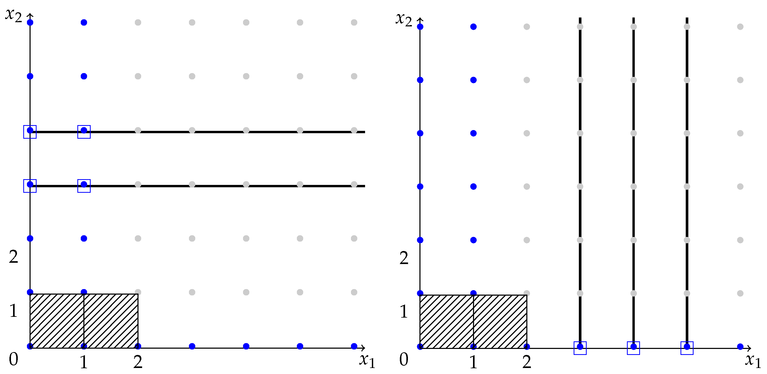
Thus, the recurrence relation between the sections involves initial data function at points $(0,x_2),(1,x_2),(0,x_2+1),(1,x_2+1),(0,x_2+2),(1,x_2+2)$, see Figure 3, the left side.

Multiplying the left-hand side of

$$\begin{array}{c}\left[(c_{00}+c_{01}{\delta }_2)+(c_{10}+c_{11}{\delta }_2){\delta }_1+(c_{20}+c_{21}{\delta }_2){\delta }_1^2\right]f(x_1,x_2)=0.\end{array}$$

(8)

by ${\xi }_2^{x_2+1}{z}_2^{\underline{{\ell }_2(x_2+1)}}$ and summing over $x_2⩾0$ yields

$$\begin{array}{c}{\displaystyle \sum _{x_2=0}^{\infty }}\left[(c_{00}+c_{01}{\delta }_2)+(c_{10}+c_{11}{\delta }_2){\delta }_1+(c_{20}+c_{21}{\delta }_2){\delta }_1^2\right]f(x_1,x_2){\xi }_2^{x_2+1}{z}_2^{\underline{{\ell }_2(x_2+1)}}\\ ={\displaystyle \sum _{x_2=0}^{\infty }}(c_{00}+c_{01}{\delta }_2)f(x_1,x_2){\xi }_2^{x_2+1}{z}_2^{\underline{{\ell }_2(x_2+1)}}\\ +{\displaystyle \sum _{x_2=0}^{\infty }}(c_{10}+c_{11}{\delta }_2)f(x_1+1,x_2){\xi }_2^{x_2+1}{z}_2^{\underline{{\ell }_2(x_2+1)}}\\ +{\displaystyle \sum _{x_2=0}^{\infty }}(c_{20}+c_{21}{\delta }_2)f(x_1+2,x_2){\xi }_2^{x_2+1}{z}_2^{\underline{{\ell }_2(x_2+1)}}\\ =c_{00}{\displaystyle \sum _{x_2=0}^{\infty }}f(x_1,x_2){\xi }_2^{x_2+1}{z}_2^{\underline{{\ell }_2(x_2+1)}}+c_{01}{\displaystyle \sum _{x_2=0}^{\infty }}f(x_1,x_2+1){\xi }_2^{x_2+1}{z}_2^{\underline{{\ell }_2(x_2+1)}}\\ +c_{10}{\displaystyle \sum _{x_2=0}^{\infty }}f(x_1+1,x_2){\xi }_2^{x_2+1}{z}_2^{\underline{{\ell }_2(x_2+1)}}+c_{11}{\displaystyle \sum _{x_2=0}^{\infty }}f(x_1+1,x_2+1){\xi }_2^{x_2+1}{z}_2^{\underline{{\ell }_2(x_2+1)}}\\ +c_{20}{\displaystyle \sum _{x_2=0}^{\infty }}f(x_1+2,x_2){\xi }_2^{x_2+1}{z}_2^{\underline{{\ell }_2(x_2+1)}}+c_{21}{\displaystyle \sum _{x_2=0}^{\infty }}f(x_1+2,x_2+1){\xi }_2^{x_2+1}{z}_2^{\underline{{\ell }_2(x_2+1)}}\\ =c_{00}{\xi }_2{z}_2^{\underline{{\ell }_2}}{\rho }_2^{{\ell }_2}{\displaystyle \sum _{x_2=0}^{\infty }}f(x_1,x_2){\xi }_2^{x_2}{z}_2^{\underline{{\ell }_2{x}_2}}+c_{01}{\displaystyle \sum _{x_2=1}^{\infty }}f(x_1,x_2){\xi }_2^{x_2}{z}_2^{\underline{{\ell }_2{x}_2}}\\ +c_{10}{\xi }_2{z}_2^{\underline{{\ell }_2}}{\rho }_2^{{\ell }_2}{\displaystyle \sum _{x_2=0}^{\infty }}f(x_1+1,x_2){\xi }_2^{x_2}{z}_2^{\underline{{\ell }_2{x}_2}}+c_{11}{\displaystyle \sum _{x_2=1}^{\infty }}f(x_1+1,x_2){\xi }_2^{x_2}{z}_2^{\underline{{\ell }_2{x}_2}}\\ +c_{20}{\xi }_2{z}_2^{\underline{{\ell }_2}}{\rho }_2^{{\ell }_2}{\displaystyle \sum _{x_2=0}^{\infty }}f(x_1+2,x_2){\xi }_2^{x_2}{z}_2^{\underline{{\ell }_2{x}_2}}+c_{21}{\displaystyle \sum _{x_2=1}^{\infty }}f(x_1+2,x_2){\xi }_2^{x_2}{z}_2^{\underline{{\ell }_2{x}_2}}\\ =c_{00}{\xi }_2{z}_2^{\underline{{\ell }_2}}{\rho }_2^{{\ell }_2}F({\xi }_2;{\ell }_2;z_2;x_1)+c_{01}\left(F({\xi }_2;{\ell }_2;z_2;x_1)-f(x_1,0)\right)\\ +c_{10}{\xi }_2{z}_2^{\underline{{\ell }_2}}{\rho }_2^{{\ell }_2}F({\xi }_2;{\ell }_2;z_2;x_1+1)+c_{11}\left(F({\xi }_2;{\ell }_2;z_2;x_1+1)-f(x_1+1,0)\right)\\ +c_{20}{\xi }_2{z}_2^{\underline{{\ell }_2}}{\rho }_2^{{\ell }_2}F({\xi }_2;{\ell }_2;z_2;x_1+2)+c_{21}\left(F({\xi }_2;{\ell }_2;z_2;x_1+2)-f(x_1+2,0)\right)\\ =\left[(c_{00}{\xi }_2{z}_2^{\underline{{\ell }_2}}{\rho }_2^{{\ell }_2}+c_{01})+(c_{10}{\xi }_2{z}_2^{\underline{{\ell }_2}}{\rho }_2^{{\ell }_2}+c_{11}){\delta }_1+(c_{20}{\xi }_2{z}_2^{\underline{{\ell }_2}}{\rho }_2^{{\ell }_2}+c_{21}){\delta }_1^2\right]F({\xi }_2;{\ell }_2;z_2;x_1)\\ -c_{01}f(x_1,0)-c_{11}f(x_1+1,0)-c_{21}f(x_1+2,0).\end{array}$$

Since the right-hand side equals zero, we get the recurrence relation for the following sections:

$$\begin{array}{c}\left[(c_{00}{\xi }_2{z}_2^{\underline{{\ell }_2}}{\rho }_2^{{\ell }_2}+c_{01})+(c_{10}{\xi }_2{z}_2^{\underline{{\ell }_2}}{\rho }_2^{{\ell }_2}+c_{11}){\delta }_1+(c_{20}{\xi }_2{z}_2^{\underline{{\ell }_2}}{\rho }_2^{{\ell }_2}+c_{21}){\delta }_1^2\right]F({\xi }_2;{\ell }_2;z_2;x_1)\\ =c_{01}\phi (x_1,0)+c_{11}\phi (x_1+1,0)+c_{21}\phi (x_1+2,0).\end{array}$$

Thus, the recurrence relation between the sections involves initial data function at points $(x_1,0),(x_1+1,0),(x_2+2,0)$, see Figure 3, the right side.

5. Conclusions

This study investigated the properties of D-finite discrete generating functions and their role in formulating recurrence relations for their sections. We showed that these sections satisfy linear recurrence relations with polynomial coefficients, thereby extending existing techniques for transforming difference equations into functional equations. Explicit recurrence relations were derived for two-dimensional generating functions, with generalizations to multidimensional cases, including those with variable coefficients.

The results have broad applications in combinatorics, where they offer a structured framework for counting constrained lattice paths and solving polynomial summation problems [25]. In computational mathematics, the derived recurrence relations enhance symbolic summation algorithms and support efficient computation methods for discrete recursive filters, which are widely used in signal processing and control systems [26,27,28,29,30].

Beyond these theoretical contributions, the results provide practical tools for combinatorial enumeration, symbolic summation, and the efficient analysis of multidimensional difference equations. Potential applications include the design of discrete recursive filters in signal processing and control theory, as well as methods for analyzing lattice paths and recurrent sequences in number theory. Future research directions involve extending the approach to nonlinear recurrences, developing algorithms for large-scale symbolic computation, and exploring connections with asymptotic analysis, big data processing, and AI-driven sequence modeling.

References

1. Stanley, R.P. Differentiably Finite Power Series. Eur. J. Comb. 1980, 1, 175–188. [Google Scholar] [CrossRef]
2. Lipshitz, L. D-Finite Power Series. J. Algebra 1989, 122, 353–373. [Google Scholar] [CrossRef]
3. Leinartas, E.; Yakovleva, T. The Cauchy Problem for Multidimensional Difference Equations and the Preservation of the Hierarchy of Generating Functions of Its Solutions. J. Sib. Fed. Univ. Math. Phys. 2018, 11, 712–722. [Google Scholar] [CrossRef]
4. Akhtamova, S.S.; Alekseev, V.S.; Lyapin, A.P. Discrete Generating Functions. Math. Notes 2023, 114, 1087–1093. [Google Scholar] [CrossRef]
5. Akhtamova, S.; Cuchta, T.; Lyapin, A. An Approach to Multidimensional Generating Series. Mathematics 2024, 12, 143. [Google Scholar] [CrossRef]
6. Bohner, M.; Cuchta, T. The Generalized Hypergeometric Difference Equation. Demonstr. Math. 2018, 51, 62–75. [Google Scholar] [CrossRef]
7. Bohner, M.; Cuchta, T. The Bessel Difference Equation. Proc. Am. Math. Soc. 2017, 145, 1567–1580. [Google Scholar] [CrossRef]
8. Bohner, M.; Peterson, A. Dynamic Equations on Time Scales: An Introduction with Applications; Birkhäuser: Boston, MA, USA, 2001. [Google Scholar]
9. Riordan, J. Combinatorial Identities; John Wiley & Sons: New York, NY, USA, 1968. [Google Scholar]
10. Bousquet-Mélou, M.; Petkovšek, M. Linear Recurrences with Constant Coefficients: The Multivariate Case. Discret. Math. 2000, 225, 51–75. [Google Scholar] [CrossRef]
11. Trishin, P.V. Necessary and Sufficient Conditions for the Existence of Rational Solutions to Homogeneous Difference Equations with Constant Coefficients. Bull. Irkutsk State Univ. Ser. Math. 2024, 47, 47–62. [Google Scholar] [CrossRef]
12. Apanovich, M.S.; Leinartas, E.K. Correctness of a Two-Dimensional Cauchy Problem for a Polynomial Difference Operator with Constant Coefficients. J. Sib. Fed. Univ. Math. Phys. 2017, 10, 199–205. [Google Scholar] [CrossRef]
13. Chandragiri, S. Counting Lattice Paths by Using Difference Equations with Non-constant Coefficients. Bull. Irkutsk State Univ. Ser. Math. 2023, 44, 55–70. [Google Scholar] [CrossRef]
14. Leinartas, E.K.; Passare, M.; Tsikh, A.K. Multidimensional Versions of Poincaré’s Theorem for Difference Equations. Sb. Math. 2008, 199, 1505–1521. [Google Scholar] [CrossRef]
15. Krasikov, V.A. A Survey on Computational Aspects of Polynomial Amoebas. Math. Comput. Sci. 2023, 17, 16. [Google Scholar] [CrossRef]
16. Leinartas, E.; Nekrasova, T. Constant Coefficient Linear Difference Equations on the Rational Cones of the Integer Lattice. Sib. Math. J. 2016, 57, 74–85. [Google Scholar] [CrossRef]
17. Lyapin, A.; Akhtamova, S. Recurrence Relations for the Sections of the Generating Series of the Solution to the Multidimensional Difference Equation. Vestn. Udmurtsk. Univ. Mat. Mekh. Komp. Nauki 2021, 31, 414–423. [Google Scholar] [CrossRef]
18. Lyapin, A.; Cuchta, T. Sections of the Generating Series of a Solution to the Multidimensional Difference Equation. Bull. Irkutsk State Univ. Ser. Math. 2022, 42, 75–89. [Google Scholar] [CrossRef]
19. Luzón, A.; Morón, M.A. Recurrence Relations for Polynomial Sequences via Riordan Matrices. Linear Algebra Appl. 2010, 433, 1422–1446. [Google Scholar] [CrossRef]
20. Andrica, D.; Bagdasar, O. Some Remarks on the Coefficients of Cyclotomic Polynomials. In New Frontiers in Number Theory and Applications; Trends in Mathematics; Guàrdia, J., Minculete, N., Savin, D., Vela, M., Zekhnini, A., Eds.; Birkhäuser: Cham, Switzerland, 2023. [Google Scholar] [CrossRef]
21. Kızılateş, C.; Polatlı, E.; Terzioğlu, N.; Du, W.-S. On Higher-Order Generalized Fibonacci Hybrid Numbers with q-Integer Components: New Properties, Recurrence Relations, and Matrix Representations. Symmetry 2025, 17, 584. [Google Scholar] [CrossRef]
22. Kostić, M.; Koyuncuoğlu, H.C. Multi-Dimensional Almost Automorphic Type Sequences and Applications. Georgian Math. J. 2024, 31, 453–471. [Google Scholar] [CrossRef]
23. Kostić, M. Almost Periodic Type Solutions to Integro-Differential-Difference Equations; De Gruyter: Berlin, Germany, 2025. [Google Scholar]
24. Leinartas, E.K.; Shishkina, O.A. The Euler–Maclaurin Formula in the Problem of Summation over Lattice Points of a Simplex. J. Sib. Fed. Univ. Math. Phys. 2022, 15, 108–113. [Google Scholar] [CrossRef]
25. Grigoriev, A.A.; Leinartas, E.K.; Lyapin, A.P. Summation of Functions and Polynomial Solutions to a Multidimensional Difference Equation. J. Sib. Fed. Univ. Math. Phys. 2023, 16, 153–161. [Google Scholar]
26. Kruchinin, D.; Kruchinin, V.; Shablya, Y. On some properties of generalized Narayana numbers. Quaest. Math. 2021, 45, 1949–1963. [Google Scholar] [CrossRef]
27. Shabiya, Y.; Kruchinin, V.; Kruchinin, D. Enumeration of Words Derived from Unambiguous Context-Free Grammars Based on Powers of Generating Functions. Proc. Jangjeon Math. Soc. 2025, 28, 299–317. [Google Scholar] [CrossRef]
28. Abramov, S.A.; Barkatou, M.A.; van Hoeij, M.; Petkovsek, M. Subanalytic Solutions of Linear Difference Equations and Multidimensional Hypergeometric Sequences. J. Symb. Comput. 2011, 46, 1205–1228. [Google Scholar] [CrossRef]
29. Abramov, S.A.; Barkatou, M.A.; Petkovšek, M. Linear Difference Operators with Coefficients in the Form of Infinite Sequences. Comput. Math. Math. Phys. 2021, 61, 1582–1589. [Google Scholar] [CrossRef]
30. Abramov, S.A.; Petkovsek, M.; Ryabenko, A.A. Hypergeometric Solutions of First-order Linear Difference Dystems with Rational-function Coefficients. In International Workshop on Computer Algebra in Scientific Computing; Lecture Notes in Computer Science; Springer International Publishing: Cham, Switzerland, 2015; Volume 9301, pp. 1–14. [Google Scholar] [CrossRef]
Figure 1. Examples of subsets of Z 2 defined by the inequalities x m , 0 x m , and x m .
Mathematics 13 03259 g001
Figure 2. Newton polytopes for the difference equations from Example 1.
Mathematics 13 03259 g002
Figure 3. Functional relations for sections of discrete generating sections from Example 3 includes values of the initial data function φ ( x ) .
Mathematics 13 03259 g003
Disclaimer/Publisher’s Note: The statements, opinions and data contained in all publications are solely those of the individual author(s) and contributor(s) and not of MDPI and/or the editor(s). MDPI and/or the editor(s) disclaim responsibility for any injury to people or property resulting from any ideas, methods, instructions or products referred to in the content.