Article

Perspectives on Dynamic Hardy–Littlewood Inequalities in Time Scale Analysis

1
Department of Mathematics, College of Science, University of Ha’il, Ha’il 2440, Saudi Arabia
2
Section of Mathematics, International Telematic University Uninettuno, Corso Vittorio Emanuele II, 39, 00186 Rome, Italy
3
Department of Mathematics, Faculty of Science, Mansoura University, Mansoura 35516, Egypt
4
Department of Basic Sciences, Faculty of Engineering Technology, El Sewedy University of Technology, Cairo 44916, Egypt
5
Department of Computing, Mathematics and Electronics, 1 Decembrie 1918 University of Alba Iulia, 510009 Alba Iulia, Romania
6
Faculty of Mathematics and Computer Science, Transilvania University of Brasov, Iuliu Maniu Street 50, 500091 Brasov, Romania
7
Department of Mathematics, Faculty of Science, Al-Azhar University, Cairo 11884, Egypt
*
Author to whom correspondence should be addressed.
Mathematics 2025, 13(13), 2176; https://doi.org/10.3390/math13132176
Submission received: 11 May 2025 / Revised: 23 June 2025 / Accepted: 29 June 2025 / Published: 3 July 2025
(This article belongs to the Special Issue Recent Advances in Dynamic Equations on Time Scales)

Abstract

This study demonstrates several novel dynamic inequalities of the Hardy and Littlewood types on time scales. As special cases, our studies include Hardy’s integral inequalities and Hardy and Littlewood’s discrete inequalities. The research findings are demonstrated using algebraic inequalities, Hölder’s inequality, and the chain rule on time scales.

1. Introduction

The study of inequalities has been a cornerstone of mathematical analysis, providing essential tools for understanding the behavior of functions across various domains. Among these, Hardy-type inequalities, introduced by G.H. Hardy in the early 20th century, have played a pivotal role in both discrete and continuous settings. These inequalities offer bounds on sums and integrals of functions, with applications spanning functional analysis, partial differential equations, and probability theory. The Hardy–Littlewood inequalities, which generalize Hardy’s original results, further extend these bounds by incorporating additional parameters, enhancing their flexibility and applicability. In 1920, Hardy [1] established the following result.
Theorem 1. 
For a sequence { κ ( ς ) } ς = 1 of non-negative terms, if ϱ > 1 , then
ς = 1 1 ς ϱ o = 1 ς κ ( o ) ϱ ϱ ϱ 1 ϱ ς = 1 κ ϱ ( ς ) .
In 1925, the continuous version of (1) was presented by Hardy [2], as seen in the result below.
Theorem 2. 
Let ϖ be a non-negative function continuous on [ 0 , ) . If ϱ > 1 , then
0 1 ϱ 0 ϖ ( ) d ϱ d ϱ ϱ 1 ϱ 0 ϖ ϱ ( ) d .
where ( ϱ / ( ϱ 1 ) ) ϱ is the best possible.
In 1927, Hardy and Littlewood [3] showed the following generalization of (1).
Theorem 3. 
For a sequence { κ ( ς ) } ς = 1 of positive terms, if ϱ > 1 , then
ς = 1 1 ς χ o = 1 ς κ ( o ) ϱ C ( ϱ , χ ) ς = 1 1 ς χ ϱ κ ϱ ( ς ) , for χ > 1 ,
and
ς = 1 1 ς χ o = ς κ ( o ) ϱ C ( ϱ , χ ) ς = 1 1 ς χ ϱ κ ϱ ( ς ) , for χ < 1 ,
where C ( ϱ , χ ) is a positive constant that depends on ϱ and χ.
In 1928, Hardy [4] established the following generalization of (2).
Theorem 4. 
Let ϖ be a non-negative function continuous on [ 0 , ) . If ϱ > 1 , then
0 1 χ 0 ϖ ( ) d ϱ d ϱ χ 1 ϱ 0 ϱ χ ϖ ϱ ( ) d , for χ > 1 ,
and
0 1 χ ϖ ( ) d ϱ d ϱ 1 χ ϱ 0 ϱ χ ϖ ϱ ( ) d , for χ < 1 .
The advent of time scale calculus, pioneered by Stefan Hilger in 1988 [5], has opened new avenues for unifying discrete and continuous analysis. Time scales provide a framework where both continuous (e.g., R ) and discrete (e.g., Z ) domains, as well as hybrid structures, can be analyzed under a single formalism. This unification is particularly valuable for studying dynamic inequalities, where traditional discrete and continuous Hardy-type inequalities can be expressed as special cases of a more general form. For more insights into Hardy-type inequalities, we recommend o the reader the papers [6,7,8,9] and the books [10,11]. In 2005, Řehák [12] obtained a time scale version of Hardy inequalities (1) and (2), unifying them into one form, as indicated in the following.
Theorem 5. 
Let T be a time scale, and ϖ C r d ( [ ι , ) T , [ 0 , ) ) , and define
Θ ( ) : = ι ϖ ( ) Δ , f o r [ ι , ) T .
If ϱ > 1 , then
ι Θ σ ( ) σ ( ) ι ϱ Δ < ϱ ϱ 1 ϱ ι ϖ ϱ ( ) Δ ,
unless ϖ 0 .
In addition, if μ ( ) / 0 as , then the constant is the best possible.
Řehák is considered the first person to generalize Hardy’s inequality on time scales. After that, many authors established several generalizations of the dynamic Hardy inequality. For more of the dynamic inequalities of Hardy type on time scales, the reader can look to the book [13] and the papers [14,15,16,17,18,19,20,21,22]. The motivation for this work lies in extending the classical Hardy and Hardy–Littlewood inequalities to time scales, thereby creating a versatile framework that captures both existing results and new generalizations. Such extensions are crucial for applications in dynamic equations, where systems may evolve on non-uniform or mixed time domains, such as in signal processing, control theory, and mathematical biology. For instance, these inequalities can bound energy dissipation in signal processing and ensure stability in control systems or model population decay in mathematical biology. This paper aims to establish novel dynamic Hardy and Littlewood-type inequalities on time scales, leveraging tools such as the Hölder inequality, chain rules, and algebraic inequalities. The results presented here not only unify and generalize previous findings but also pave the way for further exploration of dynamic inequalities in applied mathematics. The goal of this research is to establish novel dynamic Hardy and Littlewood-type inequalities on time scales. Discrete and integral inequalities are presented as special cases. This paper is structured as follows: In Section 2, we introduce fundamental concepts of calculus on time scales. In Section 3, we state and prove our main results. In Section 4, we explore applications and examples of these inequalities in areas such as stability analysis. In Section 5, we provide the discussion and conclusions of this paper.

2. Preliminaries on Time Scales

A time scale T is an arbitrary nonempty closed subset of R . We define the forward jump operator σ : T T for T by σ ( ) : = inf { T : > } . The graininess function μ : T [ 0 , ) is defined by μ ( ) : = σ ( ) . A function ϖ : T R is called rd-continuous if it is continuous at right-dense points in T and its left-sided limits exist and are finite at left-dense points in T . The set of all rd-continuous functions is denoted by C r d = C r d ( T ) = C r d ( T , R ) . For a function ϖ : T R , we define the derivative ϖ Δ as follows. Assume T . If for all ε > 0 there exists a neighborhood U of with
| ϖ ( σ ( ) ) ϖ ( ) ϖ Δ ( σ ( ) ) | ε | σ ( ) ) | , for all U ,
then ϖ Δ is said to be the delta derivative of ϖ at . As for delta integration by parts on time scales, it takes the following formula:
ν 1 ν 2 x σ ( ) y Δ ( ) Δ = x ( ) y ( ) | ν 1 ν 2 ν 1 ν 2 x Δ ( ) y ( ) Δ .
The important relations listed below were used as special instances in our studies.
If T = R , then
σ ( ) = , μ ( ) = 0 , ϖ Δ ( ) = ϖ ( ) , ν 1 ν 2 ϖ ( ) Δ = ν 1 ν 2 ϖ ( ) d .
If T = Z , then
σ ( ) = + 1 , μ ( ) = 1 , ϖ Δ ( ) = Δ ϖ ( ) , ν 1 ν 2 ϖ ( ) Δ = = ν 1 ν 2 1 ϖ ( ) .
If T = h Z = { = h z : z Z } , where h > 0 , then
σ ( ) = + h , μ ( ) = h , ϖ Δ ( ) = ϖ ( + h ) ϖ ( ) h , ν 1 ν 2 ϖ ( ) Δ = z = ν 1 h ν 2 h 1 h ϖ ( h z ) .
If T = q Z ¯ = { = q z : z Z } { 0 } , where q > 1 , then
σ ( ) = q , μ ( ) = ( q 1 ) , ϖ Δ ( ) = ϖ ( q ) ϖ ( ) ( q 1 ) , ν 1 ν 2 ϖ ( ) Δ = ( q 1 ) z = log q ν 1 log q ν 2 1 q z ϖ ( q z ) .
Lemma 1 
([23], p. 139). If ϖ and ϖ Δ are continuous, then
ι ϖ ( , ) Δ Δ = ϖ ( σ ( ) , ) + ι ϖ Δ ( , ) Δ ,
where ϖ Δ ( , ) is the delta derivative of ϖ ( , ) with respect to ℏ (for fixed ℓ).
Lemma 2 
([24], p. 32). Consider ϖ : R R , which is a continuously differentiable function, and ω : T R , which is a delta differentiable function. Then
( ϖ ω ) Δ ( ) = 0 1 ϖ h g σ ( ) + ( 1 h ) ω ( ) d h ω Δ ( ) .
Utilizing the fact that ω ( σ ( ) ) = ω ( ) + μ ( ) ω Δ ( ) , the previous chain rule Formula (14) can be written in the following form.
( ϖ ω ) Δ ( ) = 0 1 ϖ ω ( ) + h μ ( ) ω Δ ( ) d h ω Δ ( ) .
Lemma 3 
([24], p. 259). Assume ν 1 , ν 2 T and ϖ , ω C r d ( [ ν 1 , ν 2 ] T , [ 0 , ) ) . If ϱ , q > 1 such that 1 / ϱ + 1 / q = 1 , then
ν 1 ν 2 | ϖ ( ) ω ( ) | Δ ν 1 ν 2 | ϖ ( ) | ϱ Δ 1 ϱ ν 1 ν 2 | ω ( ) | q Δ 1 q .
Lemma 4 
([25], p. 51). For any ν 1 , ν 2 0 , we have the following:
( ν 1 r + ν 2 r ) ( ν 1 + ν 2 ) r 2 r 1 ( ν 1 r + ν 2 r ) , r 1 ,
and
2 r 1 ( ν 1 r + ν 2 r ) ( ν 1 + ν 2 ) r ( ν 1 r + ν 2 r ) , 0 r 1 .

3. Main Results

Throughout this paper, we assume that any time scale above is unbounded, functions are non-negative, and the improper integrals are convergent. In the following, we applied the chain rules (14) and (15) as well as the inequalities (17) and (18) to establish novel dynamic inequalities of Hardy and Littlewood type.
Lemma 5. 
Assume T is a time scale with ι [ 0 , ) T and ω C r d ( ( ι , ) T , [ 0 , ) ) and define
Θ ( ) : = ι ω ( ) Δ , for ( ι , ) T .
If ϱ 2 ( or ϱ 2 ) and χ > 1 , then, using integration by parts with u Δ ( ) = 1 ( σ ( ) ι ) χ and v σ ( ) = ( Θ σ ( ) ) ϱ , and defining u ( ) = 1 ( σ ( ) ι ) χ Δ , we have
ι ( Θ σ ( ) ) ϱ ( σ ( ) ι ) χ Δ 1 χ 1 ι ( Θ ϱ ( ) ) Δ ( ι ) χ 1 Δ .
To ensure convergence of the integrals, we assume that ω satisfies ι ω ϱ ( ) Δ < , and the interval ( ι , ) T excludes = ι to avoid singularities when χ > 1 , particularly on right-dense time scales.
Proof. 
Apply integration by parts (8) with u Δ ( ) = 1 ( σ ( ) ι ) χ and v σ ( ) = ( Θ σ ( ) ) ϱ , so that v ( ) = ( Θ ( ) ) ϱ and u ( ) = 1 ( σ ( ) ι ) χ Δ . This yields
ι Θ σ ( ) ϱ σ ( ) ι χ Δ = u ( ) Θ ( ) ϱ | ι + ι u ( ) Θ ϱ ( ) Δ Δ ,
Since Θ ( ι ) = 0 and u ( ) = 0 (as the improper integral converges), the boundary term vanishes. Using the chain rule (14) to bound u ( ) , we compute
1 ( ι ) χ 1 Δ = ( 1 χ ) 0 1 h ( σ ( ) ι ) + ( 1 h ) ( ι ) χ d h = ( χ 1 ) 0 1 d h h ( σ ( ) ι ) + ( 1 h ) ( ι ) χ ( χ 1 ) 0 1 d h h ( σ ( ) ι ) + ( 1 h ) ( σ ( ) ι ) χ = χ 1 ( σ ( ) ι ) χ 0 1 d h = χ 1 ( σ ( ) ι ) χ .
since σ ( ) . Thus,
1 ( ι ) χ 1 Δ χ 1 ( σ ( ) ι ) χ .
Divide (23) by χ 1 > 0 :
1 χ 1 1 ( ι ) χ 1 Δ 1 ( σ ( ) ι ) χ ,
and then multiply (24) by 1 , reversing the inequality:
1 χ 1 1 ( ι ) χ 1 Δ 1 ( σ ( ) ι ) χ .
Integrate (25) from ℏ to ∞, and then multiply by 1 again; thus we get u ( ) :
u ( ) = 1 σ ( ) ι χ Δ 1 χ 1 1 ( ι ) χ 1 Δ Δ = 1 χ 1 1 ( ι ) χ 1 .
Substituting into the integral (21), we obtain the desired result (20). □
The following table (Table 1) summarizes the application of Lemma 5 in the next theorems.
Theorem 6. 
Under the assumptions of Lemma 5, if ϱ 2 and χ > 1 , then
ι Θ σ ( ) ϱ σ ( ) ι χ Δ 2 ϱ 1 χ 1 ϱ ι σ ( ) ι χ ( ϱ 1 ) ι ϱ ( χ 1 ) ϖ ϱ ( ) Δ .
Proof. 
From Lemma 5, inequality (20), applying chain rule (14) to Θ ϱ ( ) Δ , we obtain
Θ ϱ ( ) Δ = ϱ 0 1 h ( Θ σ ( ) ) + ( 1 h ) Θ ( ) ϱ 1 d h Θ Δ ( ) ,
Since Θ Δ ( ) = ϖ ( ) by (13) and ϖ ( ) 0 by assumption, it follows that
Θ ϱ ( ) Δ = ϱ ϖ ( ) 0 1 h ( Θ σ ( ) ) + ( 1 h ) Θ ( ) ϱ 1 d h .
Applying the inequality (17) on the term h ( Θ σ ( ) ) + ( 1 h ) Θ ( ) ϱ 1 , we get for ϱ 2 that
Θ ϱ ( ) Δ = ϱ ϖ ( ) 0 1 h ( Θ σ ( ) ) + ( 1 h ) Θ ( ) ϱ 1 d h ϱ ϖ ( ) 0 1 2 ϱ 2 h ϱ 1 ( Θ σ ( ) ) ϱ 1 + ( 1 h ) ϱ 1 ( Θ ( ) ) ϱ 1 d h = 2 ϱ 2 ϱ ϖ ( ) 0 1 ( Θ σ ( ) ) ϱ 1 h ϱ 1 d h + 2 ϱ 2 ϱ ϖ ( ) 0 1 ( Θ ( ) ) ϱ 1 ( 1 h ) ϱ 1 d h = 2 ϱ 2 ϱ ϖ ( ) ( Θ σ ( ) ) ϱ 1 h ϱ ϱ | 0 1 2 ϱ 2 ϱ ϖ ( ) ( Θ ( ) ) ϱ 1 ( 1 h ) ϱ ϱ | 0 1 = 2 ϱ 2 ϖ ( ) ( Θ σ ( ) ) ϱ 1 + 2 ϱ 2 ϖ ( ) ( Θ ( ) ) ϱ 1 2 ϱ 2 ϖ ( ) ( Θ σ ( ) ) ϱ 1 + 2 ϱ 2 ϖ ( ) ( Θ σ ( ) ) ϱ 1 = 2 ϱ 1 ϖ ( ) ( Θ σ ( ) ) ϱ 1 .
Substituting (29) into (20), we have
ι Θ σ ( ) ϱ σ ( ) ι χ Δ 1 χ 1 ι 2 ϱ 1 ϖ ( ) ( Θ σ ( ) ) ϱ 1 ( ι ) χ 1 Δ = 2 ϱ 1 χ 1 ι ϖ ( ) ( ι ) χ 1 ( Θ σ ( ) ) ϱ 1 Δ .
Hence,
ι Θ σ ( ) ϱ σ ( ) ι χ Δ 2 ϱ 1 χ 1 ι ( σ ( ) ι ) χ ϱ 1 ϱ ( ι ) χ 1 ϖ ( ) Θ σ ( ) ϱ 1 ( σ ( ) ι ) χ ϱ 1 ϱ Δ .
Applying Hölder’s inequality (16) on the term
ι ( σ ( ) ι ) χ ϱ 1 ϱ ( ι ) χ 1 ϖ ( ) Θ σ ( ) ϱ 1 ( σ ( ) ι ) χ ϱ 1 ϱ Δ ,
with the indices ϱ and ϱ / ( ϱ 1 ) , we see that
ι ( σ ( ) ι ) χ ϱ 1 ϱ ( ι ) χ 1 ϖ ( ) Θ σ ( ) ϱ 1 ( σ ( ) ι ) χ ϱ 1 ϱ Δ ι ( σ ( ) ι ) χ ϱ 1 ϱ ( ι ) χ 1 ϖ ( ) ϱ Δ 1 ϱ ι Θ σ ( ) ϱ 1 ( σ ( ) ι ) χ ϱ 1 ϱ ϱ ϱ 1 Δ ϱ 1 ϱ .
Substituting (32) into (31) gives
ι Θ σ ( ) ϱ σ ( ) ι χ Δ 2 ϱ 1 χ 1 ι ( σ ( ) ι ) χ ϱ 1 ϱ ( ι ) χ 1 ϖ ( ) ϱ Δ 1 ϱ × ι Θ σ ( ) ϱ 1 ( σ ( ) ι ) χ ϱ 1 ϱ ϱ ϱ 1 Δ ϱ 1 ϱ .
Dividing both sides by the term ι ( Θ σ ( ) ) ϱ 1 ( ( σ ( ) ι ) χ ) ( ϱ 1 ) / ϱ ϱ / ( ϱ 1 ) Δ ( ϱ 1 ) / ϱ , and then taking both sides to the power ϱ , we see that
ι Θ σ ( ) ϱ σ ( ) ι χ Δ 2 ϱ 1 χ 1 ϱ ι σ ( ) ι χ ( ϱ 1 ) ι ( χ 1 ) ϱ ϖ ϱ ( ) Δ ,
This shows that (27) holds. □
Corollary 1. 
If we use the fact that Θ Δ ( ) 0 , then we get that
ι Θ ( ) ϱ σ ( ) ι χ Δ ι Θ σ ( ) ϱ σ ( ) ι χ Δ .
From (35) and Theorem 6, this implies that
ι Θ ( ) ϱ σ ( ) ι χ Δ 2 ϱ 1 χ 1 ϱ ι σ ( ) ι χ ( ϱ 1 ) ι ( χ 1 ) ϱ ϖ ϱ ( ) Δ .
Corollary 2. 
In Theorem 6, when T = R , then utilizing relations (9), we have
ι 1 ( ι ) χ ι ϖ ( ) d ϱ d 2 ϱ 1 χ 1 ϱ ι ϖ ϱ ( ) ( ι ) χ ϱ d .
Corollary 3. 
In Theorem 6 when T = h Z , then utilizing relations (11), we have
ς = ι h 1 ( h ς + h ι ) χ κ = ι h ς h ϖ ( h κ ) ϱ 2 ϱ 1 χ 1 ϱ ς = ι h ( h ς + h ι ) χ ( ϱ 1 ) ( h ς ι ) ( χ 1 ) ϱ ϖ ϱ ( h ς ) .
Corollary 4. 
In Theorem 6 when T = q Z ¯ , then utilizing relations (12), we have
ς = log q ι ( q 1 ) ϱ q ς ( q ς + 1 ι ) χ κ = log q ι ς q κ ϖ ( q κ ) ϱ 2 ϱ 1 χ 1 ϱ ς = log q ι q ς ( q ς + 1 ι ) χ ( ϱ 1 ) ( q ς ι ) ( χ 1 ) ϱ ϖ ϱ ( q ς ) .
Theorem 7. 
Under the assumptions of Lemma 5, if ϱ 2 and χ > 1 , then
ι Θ σ ( ) ϱ σ ( ) ι χ Δ 2 ϱ 2 ϱ χ 1 ι σ ( ) ι χ ( ϱ 1 ) ( ι ) ( χ 1 ) ϱ ϖ ϱ ( ) Δ 1 ϱ × ι Θ σ ( ) ϱ σ ( ) ι χ Δ ϱ 1 ϱ + 2 ϱ 2 χ 1 ι μ ϱ 1 ( ) ϖ ϱ ( ) ( ι ) χ 1 Δ .
Proof. 
From Lemma 5, inequality (20), applying chain rule (15) to Θ ϱ ( ) Δ , we obtain
Θ ϱ ( ) Δ = ϱ 0 1 Θ ( ) + h μ ( ) Θ Δ ( ) ϱ 1 d h Θ Δ ( ) ,
and since Θ Δ ( ) = ϖ ( ) 0 , we see that
Θ ϱ ( ) Δ = ϱ ϖ ( ) 0 1 Θ ( ) + h μ ( ) Θ Δ ( ) ϱ 1 d h .
Applying (17) on the term Θ ( ) + h μ ( ) Θ Δ ( ) ϱ 1 , we get for ϱ 2 that
Θ ϱ ( ) Δ = ϱ ϖ ( ) 0 1 Θ ( ) + h μ ( ) Θ Δ ( ) ϱ 1 d h ϱ ϖ ( ) 0 1 2 ϱ 2 ( Θ ( ) ) ϱ 1 + ( h ) ϱ 1 μ ( ) ϖ ( ) ϱ 1 d h = 2 ϱ 2 ϱ ϖ ( ) 0 1 ( Θ ( ) ) ϱ 1 d h + 2 ϱ 2 ϱ ϖ ( ) 0 1 ( μ ( ) ϖ ( ) ) ϱ 1 ( h ) ϱ 1 d h = 2 ϱ 2 ϱ ϖ ( ) ( Θ ( ) ) ϱ 1 ( h ) | 0 1 + 2 ϱ 2 ϱ ( μ ( ) ) ϱ 1 ( ϖ ( ) ) ϱ h ϱ ϱ | 0 1 = 2 ϱ 2 ϱ ϖ ( ) ( Θ ( ) ) ϱ 1 + 2 ϱ 2 ( μ ( ) ) ϱ 1 ( ϖ ( ) ) ϱ 2 ϱ 2 ϱ ϖ ( ) ( Θ σ ( ) ) ϱ 1 + 2 ϱ 2 ( μ ( ) ) ϱ 1 ( ϖ ( ) ) ϱ .
Substituting (38) into (20), we have
ι Θ σ ( ) ϱ σ ( ) ι χ Δ 1 χ 1 ι 2 ϱ 2 ϱ ϖ ( ) ( Θ σ ( ) ) ϱ 1 + 2 ϱ 2 μ ϱ 1 ( ) ϖ ϱ ( ) ( ι ) χ 1 Δ = 2 ϱ 2 ϱ χ 1 ι ( Θ σ ( ) ) ϱ 1 ( ι ) χ 1 ϖ ( ) Δ + 2 ϱ 2 χ 1 ι μ ϱ 1 ( ) ϖ ϱ ( ) ( ι ) χ 1 Δ .
This implies that
ι Θ σ ( ) ϱ σ ( ) ι χ Δ 2 ϱ 2 ϱ χ 1 ι ( σ ( ) ι ) χ ϱ 1 ϱ ( ι ) χ 1 ϖ ( ) ( Θ σ ( ) ) ϱ 1 ( σ ( ) ι ) χ ϱ 1 ϱ Δ + 2 ϱ 2 χ 1 ι μ ϱ 1 ( ) ϖ ϱ ( ) ( ι ) χ 1 Δ .
Applying (16) on the term
ι ( σ ( ) ι ) χ ϱ 1 ϱ ( ι ) χ 1 ϖ ( ) ( Θ σ ( ) ) ϱ 1 ( σ ( ) ι ) χ ϱ 1 ϱ Δ ,
with the indices ϱ and ϱ / ( ϱ 1 ) , gives
ι Θ σ ( ) ϱ σ ( ) ι χ Δ 2 ϱ 2 ϱ χ 1 ι ( σ ( ) ι ) χ ϱ 1 ϱ ( ι ) χ 1 ϖ ( ) ϱ Δ 1 ϱ × ι Θ σ ( ) ϱ 1 ( σ ( ) ι ) χ ϱ 1 ϱ ϱ ϱ 1 Δ ϱ 1 ϱ + 2 ϱ 2 χ 1 ι μ ϱ 1 ( ) ϖ ϱ ( ) ( ι ) χ 1 Δ ,
This shows that (36) holds. □
Corollary 5. 
If we use the fact that Θ Δ ( ) 0 and σ ( ) shown in (35), then Theorem 7 is as follows:
ι Θ ( ) ϱ σ ( ) ι χ Δ 2 ϱ 2 ϱ χ 1 ι σ ( ) ι χ ( ϱ 1 ) ( ι ) ( χ 1 ) ϱ ϖ ϱ ( ) Δ 1 ϱ × ι Θ σ ( ) ϱ σ ( ) ι χ Δ ϱ 1 ϱ + 2 ϱ 2 χ 1 ι μ ϱ 1 ( ) ϖ ϱ ( ) ( ι ) χ 1 Δ .
Corollary 6. 
Assume that T = R in Theorem 7. Then
ι 1 ( ι ) χ ι ϖ ( ) d ϱ d ϱ 2 ϱ 2 χ 1 ϱ ι ϖ ϱ ( ) ( ι ) χ ϱ d .
Corollary 7. 
Assume that T = h Z in Theorem 7. Then
ς = ι h h ϱ ( h ς + h ι ) χ κ = ι h ς ϖ ( h κ ) ϱ ϱ 2 ϱ 2 χ 1 ς = ι h ( h ς + h ι ) χ ( ϱ 1 ) ( h ς ι ) ( χ 1 ) ϱ ϖ ϱ ( h ς ) 1 ϱ × ς = ι h h ϱ ( h ς + h ι ) χ κ = ι h ς ϖ ( h κ ) ϱ ϱ 1 ϱ + 2 ϱ 2 h ϱ 1 χ 1 ς = ι h ϖ ϱ ( h ς ) ( h ς ι ) χ 1 .
Corollary 8. 
Assume that T = q Z ¯ in Theorem 7. Then
ς = log q ι ( q 1 ) ϱ q ς ( q ς + 1 ι ) χ κ = log q ι ς q κ ϖ ( q κ ) ϱ ϱ 2 ϱ 2 χ 1 ς = log q ι q ς ( q ς + 1 ι ) χ ( ϱ 1 ) ( q ς ι ) ( χ 1 ) ϱ ϖ ϱ ( q ς ) 1 ϱ × ς = log q ι ( q 1 ) ϱ q ς ( q ς + 1 ι ) χ κ = log q ι ς q κ ϖ ( q κ ) ϱ ϱ 1 ϱ + 2 ϱ 2 ( q 1 ) ϱ 1 χ 1 ς = log q ι q ς ϱ ( q ς ι ) χ 1 ϖ ϱ ( q ς ) .
Theorem 8. 
Under the assumptions of Lemma 5, if ϱ 2 and χ > 1 , then
ι Θ σ ( ) ϱ σ ( ) ι χ Δ 2 χ 1 ϱ ι σ ( ) ι χ ( ϱ 1 ) ι ( χ 1 ) ϱ ϖ ϱ ( ) Δ .
Proof. 
From Lemma 5, inequality (20), applying chain rule (14) to Θ ϱ ( ) Δ , we obtain
Θ ϱ ( ) Δ = ϱ 0 1 h ( Θ σ ( ) ) + ( 1 h ) Θ ( ) ϱ 1 d h Θ Δ ( ) ,
and since Θ Δ ( ) = ϖ ( ) 0 , we see that
Θ ϱ ( ) Δ = ϱ ϖ ( ) 0 1 h ( Θ σ ( ) ) + ( 1 h ) Θ ( ) ϱ 1 d h .
Applying (18) on the term h ( Θ σ ( ) ) + ( 1 h ) Θ ( ) ϱ 1 , we get for ϱ 2 that
Θ ϱ ( ) Δ = ϱ ϖ ( ) 0 1 h ( Θ σ ( ) ) + ( 1 h ) Θ ( ) ϱ 1 d h ϱ ϖ ( ) 0 1 h ϱ 1 ( Θ σ ( ) ) ϱ 1 + ( 1 h ) ϱ 1 ( Θ ( ) ) ϱ 1 d h = ϱ ϖ ( ) 0 1 ( Θ σ ( ) ) ϱ 1 h ϱ 1 d h + ϱ ϖ ( ) 0 1 ( Θ ( ) ) ϱ 1 ( 1 h ) ϱ 1 d h = ϱ ϖ ( ) ( Θ σ ( ) ) ϱ 1 h ϱ ϱ | 0 1 ϱ ϖ ( ) ( Θ ( ) ) ϱ 1 ( 1 h ) ϱ ϱ | 0 1 = ϖ ( ) ( Θ σ ( ) ) ϱ 1 + ϖ ( ) ( Θ ( ) ) ϱ 1 ϖ ( ) ( Θ σ ( ) ) ϱ 1 + ϖ ( ) ( Θ σ ( ) ) ϱ 1 = 2 ϖ ( ) ( Θ σ ( ) ) ϱ 1 .
Substituting (44) into (20), we have
ι Θ σ ( ) ϱ σ ( ) ι χ Δ 1 χ 1 ι 2 ϖ ( ) ( Θ σ ( ) ) ϱ 1 ( ι ) χ 1 Δ = 2 χ 1 ι ϖ ( ) ( ι ) χ 1 ( Θ σ ( ) ) ϱ 1 Δ .
This implies
ι Θ σ ( ) ϱ σ ( ) ι χ Δ 2 χ 1 ι ( σ ( ) ι ) χ ϱ 1 ϱ ( ι ) χ 1 ϖ ( ) Θ σ ( ) ϱ 1 ( σ ( ) ι ) χ ϱ 1 ϱ Δ .
Applying (16) on the term
ι ( σ ( ) ι ) χ ϱ 1 ϱ ( ι ) χ 1 ϖ ( ) Θ σ ( ) ϱ 1 ( σ ( ) ι ) χ ϱ 1 ϱ Δ ,
with the indices ϱ and ϱ / ( ϱ 1 ) , gives
ι Θ σ ( ) ϱ σ ( ) ι χ Δ 2 χ 1 ι ( σ ( ) ι ) χ ϱ 1 ϱ ( ι ) χ 1 ϖ ( ) ϱ Δ 1 ϱ × ι Θ σ ( ) ϱ 1 ( σ ( ) ι ) χ ϱ 1 ϱ ϱ ϱ 1 Δ ϱ 1 ϱ .
Dividing both sides by ι ( Θ σ ( ) ) ϱ 1 ( ( σ ( ) ι ) χ ) ( ϱ 1 ) / ϱ ϱ / ( ϱ 1 ) Δ ( ϱ 1 ) / ϱ and then taking to the power ϱ , we see that
ι Θ σ ( ) ϱ σ ( ) ι χ Δ 2 χ 1 ϱ ι ( σ ( ) ι ) χ ϱ 1 ϱ ( ι ) χ 1 ϖ ( ) ϱ Δ ,
This shows that (42) holds. □
Corollary 9. 
Utilizing the fact Θ Δ ( ) 0 and σ ( ) as in (35) implies that Theorem 8 is as follows:
ι Θ ( ) ϱ σ ( ) ι χ Δ 2 χ 1 ϱ ι σ ( ) ι χ ( ϱ 1 ) ι ( χ 1 ) ϱ ϖ ϱ ( ) Δ .
Corollary 10. 
Assume that T = R in Theorem 8. Then
ι 1 ( ι ) χ ι ϖ ( ) d ϱ d 2 χ 1 ϱ ι ϖ ϱ ( ) ( ι ) χ ϱ d .
Corollary 11. 
Assume that T = h Z in Theorem 8. Then
ς = ι h 1 ( h ς + h ι ) χ κ = ι h ς h ϖ ( h κ ) ϱ 2 χ 1 ϱ ς = ι h ( h ς + h ι ) χ ( ϱ 1 ) ( h ς ι ) ( χ 1 ) ϱ ϖ ϱ ( h ς ) .
Corollary 12. 
Assume that T = q Z ¯ in Theorem 8. Then
ς = log q ι ( q 1 ) ϱ q ς ( q ς + 1 ι ) χ κ = log q ι ς q κ ϖ ( q κ ) ϱ 2 χ 1 ϱ ς = log q ι q ς ( q ς + 1 ι ) χ ( ϱ 1 ) ( q ς ι ) ( χ 1 ) ϱ ϖ ϱ ( q ς ) .
Theorem 9. 
Under the assumptions of Lemma 5, if ϱ 2 and χ > 1 , then
ι Θ σ ( ) ϱ σ ( ) ι χ Δ ϱ χ 1 ι σ ( ) ι χ ( ϱ 1 ) ( ι ) ( χ 1 ) ϱ ϖ ϱ ( ) Δ 1 ϱ × ι Θ σ ( ) ϱ σ ( ) ι χ Δ ϱ 1 ϱ + 1 χ 1 ι μ ϱ 1 ( ) ϖ ϱ ( ) ( ι ) χ 1 Δ .
Proof. 
From Lemma 5, inequality (20), applying chain rule (15) to Θ ϱ ( ) Δ , we obtain
Θ ϱ ( ) Δ = ϱ 0 1 Θ ( ) + h μ ( ) Θ Δ ( ) ϱ 1 d h Θ Δ ( ) ,
and since Θ Δ ( ) = ϖ ( ) 0 , we see that
Θ ϱ ( ) Δ = ϱ ϖ ( ) 0 1 Θ ( ) + h μ ( ) Θ Δ ( ) ϱ 1 d h .
Applying (18) on the term Θ ( ) + h μ ( ) Θ Δ ( ) ϱ 1 , we get for ϱ 2 that
Θ ϱ ( ) Δ = ϱ ϖ ( ) 0 1 Θ ( ) + h μ ( ) Θ Δ ( ) ϱ 1 d h ϱ ϖ ( ) 0 1 ( Θ ( ) ) ϱ 1 + ( h ) ϱ 1 ( μ ( ) ϖ ( ) ) ϱ 1 d h = ϱ ϖ ( ) 0 1 ( Θ ( ) ) ϱ 1 d h + ϱ ϖ ( ) 0 1 ( μ ( ) ϖ ( ) ) ϱ 1 ( h ) ϱ 1 d h = ϱ ϖ ( ) ( Θ ( ) ) ϱ 1 ( h ) | 0 1 + ϱ ( μ ( ) ) ϱ 1 ( ϖ ( ) ) ϱ h ϱ ϱ | 0 1 = ϱ ϖ ( ) ( Θ ( ) ) ϱ 1 + ( μ ( ) ) ϱ 1 ( ϖ ( ) ) ϱ ϱ ϖ ( ) ( Θ σ ( ) ) ϱ 1 + ( μ ( ) ) ϱ 1 ( ϖ ( ) ) ϱ .
Substituting (51) into (20), we have
ι Θ σ ( ) ϱ σ ( ) ι χ Δ 1 χ 1 ι ϱ ϖ ( ) ( Θ σ ( ) ) ϱ 1 + μ ϱ 1 ( ) ϖ ϱ ( ) ( ι ) χ 1 Δ = ϱ χ 1 ι ( Θ σ ( ) ) ϱ 1 ( ι ) χ 1 ϖ ( ) Δ + 1 χ 1 ι μ ϱ 1 ( ) ϖ ϱ ( ) ( ι ) χ 1 Δ .
This implies that
ι Θ σ ( ) ϱ σ ( ) ι χ Δ ϱ χ 1 ι ( σ ( ) ι ) χ ϱ 1 ϱ ( ι ) χ 1 ϖ ( ) ( Θ σ ( ) ) ϱ 1 ( σ ( ) ι ) χ ϱ 1 ϱ Δ + 1 χ 1 ι μ ϱ 1 ( ) ϖ ϱ ( ) ( ι ) χ 1 Δ .
Applying (16) on the term
ι ( σ ( ) ι ) χ ϱ 1 ϱ ( ι ) χ 1 ϖ ( ) ( Θ σ ( ) ) ϱ 1 ( σ ( ) ι ) χ ϱ 1 ϱ Δ ,
with the indices ϱ and ϱ / ( ϱ 1 ) , we see that
ι Θ σ ( ) ϱ σ ( ) ι χ Δ ϱ χ 1 ι ( σ ( ) ι ) χ ϱ 1 ϱ ( ι ) χ 1 ϖ ( ) ϱ Δ 1 ϱ      × ι Θ σ ( ) ϱ 1 ( σ ( ) ι ) χ ϱ 1 ϱ ϱ ϱ 1 Δ ϱ 1 ϱ + 1 χ 1 ι μ ϱ 1 ( ) ϖ ϱ ( ) ( ι ) χ 1 Δ ,
This shows that (49) holds. □
Corollary 13. 
Utilizing the fact Θ Δ ( ) 0 and σ ( ) shown in (35) leads to Theorem 9 being as follows:
ι Θ ( ) ϱ σ ( ) ι χ Δ ϱ χ 1 ι σ ( ) ι χ ( ϱ 1 ) ( ι ) ( χ 1 ) ϱ ϖ ϱ ( ) Δ 1 ϱ             × ι Θ σ ( ) ϱ σ ( ) ι χ Δ ϱ 1 ϱ + 1 χ 1 ι μ ϱ 1 ( ) ϖ ϱ ( ) ( ι ) χ 1 Δ .
Corollary 14. 
Assume that T = R in Theorem 9. Then
ι 1 ( ι ) χ ι ϖ ( ) d ϱ d ϱ χ 1 ϱ ι ϖ ϱ ( ) ( ι ) χ ϱ d .
Corollary 15. 
Assume that T = h Z in Theorem 9. Then
ς = ι h h ϱ ( h ς + h ι ) χ κ = ι h ς ϖ ( h κ ) ϱ ϱ χ 1 ς = ι h ( h ς + h ι ) χ ( ϱ 1 ) ( h ς ι ) ( χ 1 ) ϱ ϖ ϱ ( h ς ) 1 ϱ          × ς = ι h h ϱ ( h ς + h ι ) χ κ = ι h ς ϖ ( h κ ) ϱ ϱ 1 ϱ + h ϱ 1 χ 1 ς = ι h ϖ ϱ ( h ς ) ( h ς ι ) χ 1 .
Corollary 16. 
Assume that T = q Z ¯ in Theorem 9. Then
ς = log q ι ( q 1 ) ϱ q ς ( q ς + 1 ι ) χ κ = log q ι ς q κ ϖ ( q κ ) ϱ ϱ χ 1 ς = log q ι q ς ( q ς + 1 ι ) χ ( ϱ 1 ) ( q ς ι ) ( χ 1 ) ϱ ϖ ϱ ( q ς ) 1 ϱ × ς = log q ι ( q 1 ) ϱ q ς ( q ς + 1 ι ) χ κ = log q ι ς q κ ϖ ( q κ ) ϱ ϱ 1 ϱ + ( q 1 ) ϱ 1 χ 1 ς = log q ι q ς ϱ ( q ς ι ) χ 1 ϖ ϱ ( q ς ) .

4. Applications

In this section, we present applications of the dynamic Hardy and Littlewood-type inequality established in Theorem 6, with a focus on its utility among the results in Theorems 6–9. These applications highlight the role of Theorem 6 in stability analysis of dynamic systems and numerical validation of its general form on the time scale. By leveraging the unified framework of time scale calculus, our inequality provides robust tools for analyzing systems across various time scales.

4.1. Stability Analysis

The dynamic inequality in Theorem 6 is a powerful tool for assessing the stability of solutions to dynamic equations on time scales. Consider a linear dynamic equation of the form
ϖ Δ ( ) = a ( ) ϖ ( ) , ( ι , ) T ,
where T is a time scale, ϖ ( ) represents the state of the system (e.g., displacement in a mechanical system or voltage in an electrical circuit), and a ( ) a 0 > 0 is a positive rd-continuous function ensuring exponential decay of the solution. The constant a 0 > 0 guarantees that ϖ ( ) approaches zero, facilitating the application of Theorem 6 to bound the system’s energy. The energy of the system is defined as ι ϖ 2 ( ) Δ , which quantifies the cumulative magnitude of the state over the time scale. For the system to be stable, this energy must be finite, indicating that the state ϖ ( ) does not grow unbounded and ideally decays to zero as . Stability is critical in applications such as control systems, where ensuring that perturbations decay over time prevents system failure, or in physical systems like damped oscillators, where energy dissipation is necessary for equilibrium. Define Θ ( ) = ι ϖ ( ) Δ , as in Theorem 6. Applying Theorem 6 with ϱ = 2 and χ = 2 , we obtain
ι Θ σ ( ) 2 ( σ ( ) ι ) 2 Δ 4 ι ( σ ( ) ι ) 2 ( ι ) 2 ϖ 2 ( ) Δ .
For T = R , since σ ( ) = by (9), this simplifies to
ι ι ϖ ( ) d 2 ( ι ) 2 d 4 ι ϖ 2 ( ) d ,
recovering the classical Hardy inequality (2). This bound ensures that the energy ι ϖ 2 ( ) Δ is finite, confirming that the system’s state decays appropriately, a hallmark of stability across various time scales.

4.2. Example

To illustrate the application of Theorem 6 and explore its behavior, we consider a specific case with parameters consistent with the stability analysis in Section 4.1. Set ϱ = 2 , χ = 2 , ι = 0 , and ϖ ( ) = e on T = R . The inequality from Theorem 6 becomes
0 0 e d 2 2 d 4 0 e 2 d .
With ϱ = 2 , χ = 2 , the constant is 2 2 1 2 1 2 = 4 . Compute the left-hand side: 0 e d = 1 e , so the integrand is ( 1 e ) 2 2 . The right-hand side integrand is 4 e 2 . Numerical evaluation from = 0.01 to 100 (avoiding the singularity at = 0 ) using adaptive quadrature yields approximately 0.644 for the left-hand side and 4 · 1 2 = 2 for the right-hand side. Since 0.644 < 2 , the inequality holds, validating Theorem 6 and aligning with the stability analysis in Section 4.1.
To further explore the behavior of Theorem 6, we visualize the integrands of the left-hand and right-hand sides of the inequality on T = R for ϱ = 2 , χ = 2 , ι = 0 , and ϖ ( ) = e . Figure 1 compares these integrands over [ 0.01 , 20 ] to capture the behavior near the origin and the crossover.
The plot shows that the right-hand side integrand eventually dominates the left-hand side, confirming that the integral of the right-hand side exceeds that of the left-hand side, as required by the inequality. Note that the left-hand side exceeds the right-hand side locally near the origin, but the integral inequality holds over [ 0 , ) , highlighting the sharpness of the constant 4, consistent with the stability properties discussed in Section 4.1.

5. Discussion and Conclusions

The results presented in this paper significantly advance the understanding of Hardy and Littlewood-type inequalities within the framework of time scale calculus. By establishing Theorems 6–9, we have generalized classical inequalities to arbitrary time scales, unifying discrete and continuous forms while introducing new dynamic inequalities. These theorems leverage the chain rules and Hölder’s inequality to derive bounds that are both robust and adaptable to various time scale structures, such as R , h Z , and q Z ¯ . The corollaries further demonstrate the versatility of our results, recovering classical Hardy and Littlewood inequalities as special cases while providing new insights for non-standard time scales. Compared to previous work, such as Řehák’s foundational time scale generalization [12] and subsequent extensions [14,18], our results introduce a broader parameter range (e.g., ϱ 2 and ϱ 2 ) and incorporate the Hardy–Littlewood framework, which allows for more flexible weighting through the parameter χ . This flexibility enhances the applicability of our inequalities to problems where the time domain exhibits hybrid behavior, such as in dynamic systems with mixed continuous and discrete evolution. Additionally, our use of algebraic inequalities (Lemma 4) provides sharper constants compared to some earlier dynamic inequalities, improving the precision of the bounds. The contributions of this work are twofold. First, it provides a unified framework that seamlessly bridges classical discrete and continuous inequalities, making it a valuable tool for researchers studying dynamic equations on time scales. Second, the new inequalities open avenues for applications in areas such as stability analysis of dynamic systems, optimization problems, and numerical methods on non-uniform grids. Future work could explore the extension of these inequalities to multi-dimensional time scales or incorporate additional functional constraints, such as convexity or monotonicity, to further refine the bounds. For example, these inequalities could be applied to partial dynamic equations on multi-dimensional time scales or extended to hybrid quantum scales for applications in quantum control systems. In conclusion, this study profoundly enriches the theoretical foundation of dynamic inequalities and establishes a versatile platform for practical applications across diverse mathematical and scientific fields. The novel inequalities introduced here highlight the transformative potential of time scale calculus in unifying and extending classical results, providing a powerful toolkit for addressing complex analytical challenges in dynamic systems, control theory, and beyond. Future research may extend these findings to nonlinear systems or hybrid time scales, further broadening their impact.

Author Contributions

Methodology, T.S.H.; Software, W.M.H.; Validation, H.M.R.; Formal analysis, I.-L.P. and H.M.R.; Investigation, T.S.H. and M.B.M.; Resources, W.M.H.; Data curation, T.S.H., W.M.H., and M.B.M.; Writing—original draft, W.M.H. and H.M.R.; Writing—review & editing, M.B.M. and A.A.; Supervision, T.S.H. and H.M.R.; Funding acquisition, I.-L.P. All authors have read and agreed to the published version of the manuscript.

Funding

This research received no external funding.

Data Availability Statement

The original contributions presented in this study are included in the article. Further inquiries can be directed to the corresponding author.

Conflicts of Interest

The authors declare no conflict of interest.

References

  1. Hardy, G.H. Note on a Theorem of Hilbert. Math. Z. 1920, 6, 314–317. [Google Scholar] [CrossRef]
  2. Hardy, G.H. Notes on some points in the integral calculus (LX). Messenger Math. 1925, 54, 150–156. [Google Scholar]
  3. Littlewood, J.E.; Hardy, G.H. Elementary Theorems concerning power series with positive coefficients and moment constants of positive functions. J. Reine Angew. Math. 1927, 157, 141–158. [Google Scholar] [CrossRef]
  4. Hardy, G.H. Notes on some points in the integral calculus (LXI). Messenger Math. 1928, 57, 12–16. [Google Scholar]
  5. Hilger, S. Analysis on measure chains—A unified approach to continuous and discrete calculus. Results Math. 1990, 18, 18–56. [Google Scholar] [CrossRef]
  6. García García, V.; Ortega Salvador, P. Some new weighted weak-type iterated and bilinear modified Hardy inequalities. Ann. Funct. Anal. 2024, 15, 26. [Google Scholar] [CrossRef]
  7. Orazbayev, A.; Suragan, D. Improved LpLq Hardy inequalities. Math. Inequal. Appl. 2024, 27, 981–990. [Google Scholar]
  8. Bianchi, F.; Brasco, L.; Sk, F.; Zagati, A.C. A note on the supersolution method for Hardy’s inequality. Rev. Mat. Complut. 2024, 37, 323–340. [Google Scholar] [CrossRef]
  9. Zakarya, M.; AlNemer, G.; El-Hamid, H.A.A.; Butush, R.; Rezk, H.M. On refinements of multidimensional inequalities of Hardy-type via superquadratic and subquadratic functions. J. Math. 2022, 2022, 7668860. [Google Scholar] [CrossRef]
  10. Kufner, A.; Maligranda, L.; Persson, L.-E. The Hardy Inequality: About Its History and Some Related Results; Vydavatelský Servis: Plzeň, Czech Republic, 2007. [Google Scholar]
  11. Persson, L.-E.; Kufner, A.; Samko, N. Weighted Inequalities of Hardy Type; World Scientific Publishing Company: Singapore, 2017. [Google Scholar]
  12. Řehák, P. Hardy inequality on time scales and its application to half-linear dynamic equations. J. Inequal. Appl. 2005, 2005, 495–507. [Google Scholar] [CrossRef]
  13. Bohner, M.; Georgiev, S.G. Multivariable Dynamic Calculus on Time Scales; Springer: Berlin/Heidelberg, Germany, 2016. [Google Scholar]
  14. Agarwal, R.P.; O’Regan, D.; Saker, S.H. Hardy Type Inequalities on Time Scales; Springer: Cham, Switzerland, 2016. [Google Scholar]
  15. Bohner, M.; Jadlovská, I.; Saied, A.I. Some new Hardy-type inequalities with negative parameters on time scales. Qual. Theory Dyn. Syst. 2025, 24, 72. [Google Scholar] [CrossRef]
  16. Kayar, Z.; Kaymakçalan, B. Converses of nabla Pachpatte-type dynamic inequalities on arbitrary time scales. Demonstr. Math. 2025, 58, 20250114. [Google Scholar] [CrossRef]
  17. Saqib, M.; Saleem, M.; Hasnain, S. New generalized extended Hardy-type dynamic inequalities on time scales. Babyl. J. Math. 2024, 2024, 178–197. [Google Scholar] [CrossRef]
  18. Aly, E.S.; Madani, Y.A.; Gassem, F.; Saied, A.I.; Rezk, H.M.; Mohammed, W.W. Some dynamic Hardy-type inequalities with negative parameters on time scales nabla calculus. AIMS Math. 2024, 9, 5147–5170. [Google Scholar] [CrossRef]
  19. Hasan, W.M.; El-Owaidy, H.M.; El-Deeb, A.A.; Rezk, H.M. A generalization of some integral inequalities similar to Hardy inequality on time scales. Kuwait J. Sci. 2024, 51, 100124. [Google Scholar] [CrossRef]
  20. Rezk, H.M.; El-Owaidy, H.M.; Hasan, W.M.; El-Deeb, A.A. Dynamic Hardy-type inequalities with convex and non-convex functions on time scales. J. Math. Sci. 2025. [Google Scholar] [CrossRef]
  21. Essam Awwad, A.; Saied, I. Some weighted dynamic inequalities of Hardy type with kernels on time scales nabla calculus. J. Math. Inequal. 2024, 18, 457–475. [Google Scholar] [CrossRef]
  22. Saker, S.H.; Mahmoud, R.R.; Osman, M.M.; Agarwal, R.P. Some new generalized forms of Hardy’s type inequality on time scales. Math. Inequal. Appl. 2017, 20, 459–481. [Google Scholar] [CrossRef]
  23. Bohner, M.; Peterson, A. Advances in Dynamic Equations on Time Scales; Birkhäuser Boston, Inc.: Boston, MA, USA, 2003. [Google Scholar]
  24. Bohner, M.; Peterson, A. Dynamic Equations on Time Scales: An Introduction with Applications; Birkhäuser Boston, Inc.: Boston, MA, USA, 2001. [Google Scholar]
  25. Agarwal, R.P.; Pang, P.Y. Opial Inequalities with Applications in Differential and Difference Equations; Springer Science & Business Media: Berlin/Heidelberg, Germany, 2013. [Google Scholar]
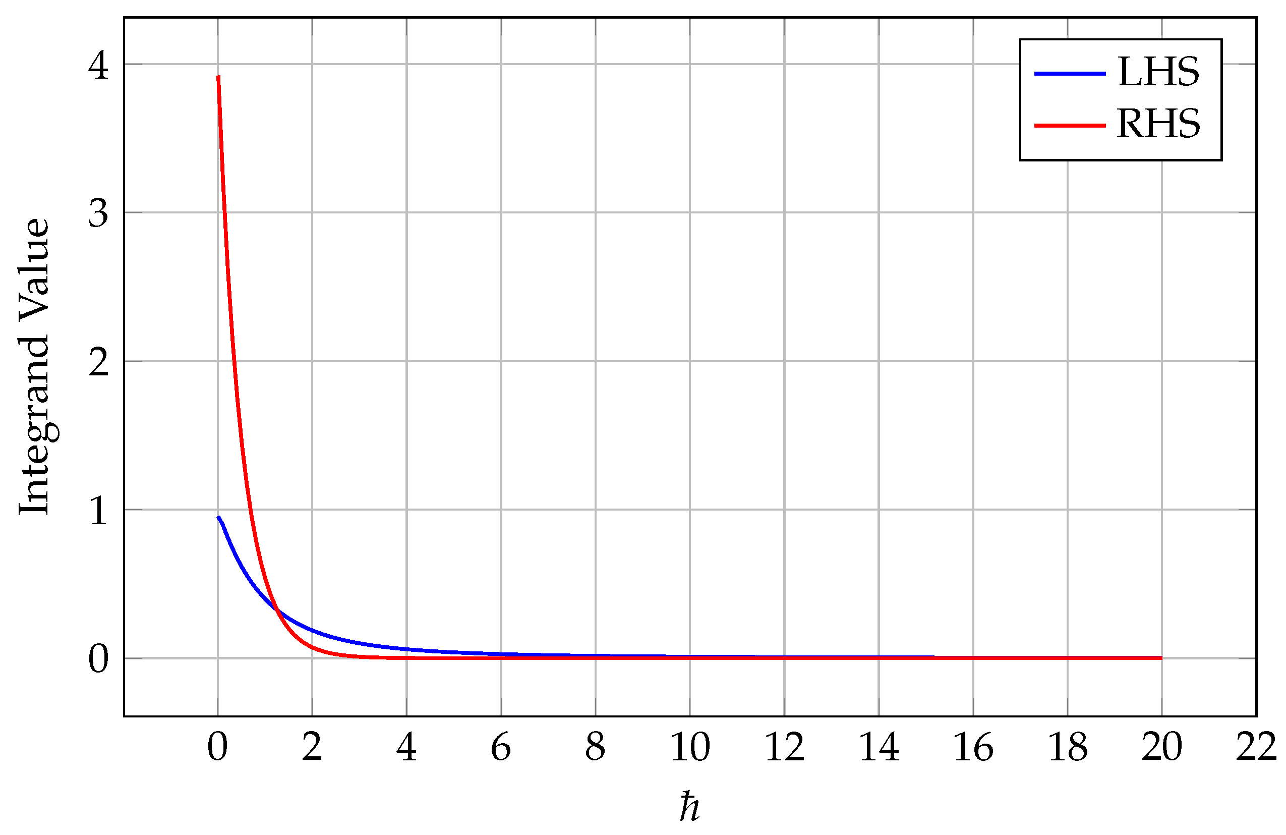
Figure 1. Comparison of the LHS and RHS integrands of (55).
Mathematics 13 02176 g001
Table 1. Key Parameters and Results for Hardy-Type Inequalities on Time Scales.
TheoremChain RuleAlgebraic BoundParameters
6(14)(17) ϱ 2 , χ > 1
7(15)(17) ϱ 2 , χ > 1
8(14)(18) ϱ 2 , χ > 1
9(15)(18) ϱ 2 , χ > 1
Disclaimer/Publisher’s Note: The statements, opinions and data contained in all publications are solely those of the individual author(s) and contributor(s) and not of MDPI and/or the editor(s). MDPI and/or the editor(s) disclaim responsibility for any injury to people or property resulting from any ideas, methods, instructions or products referred to in the content.