Abstract
Real-time lossless image compression based on the JPEG-LS algorithm is in high demand for critical missions such as satellite remote sensing and space exploration due to its excellent balance between complexity and compression rate. However, few researchers have made appropriate modifications to the JPEG-LS algorithm to make it more suitable for high-speed hardware implementation and application to Bayer pattern data. This paper addresses the current limitations by proposing a real-time lossless compression system specifically tailored for Bayer pattern images from spaceborne cameras. The system integrates a hybrid encoding strategy modified from JPEG-LS, combining run-length encoding, predictive encoding, and a non-encoding mode to facilitate high-speed hardware implementation. Images are processed in tiles, with each tile’s color channels processed independently to preserve individual channel characteristics. Moreover, potential error propagation is confined within a single tile. To enhance throughput, the compression algorithm operates within a 20-stage pipeline architecture. Duplication of computation units and the introduction of key-value registers and a bypass mechanism resolve structural and data dependency hazards within the pipeline. A reorder architecture prevents pipeline blocking, further optimizing system throughput. The proposed architecture is implemented on a XILINX XC7Z045-2FFG900C SoC (Xilinx, Inc., San Jose, CA, USA) and achieves a maximum throughput of up to 346.41 MPixel/s, making it the fastest architecture reported in the literature.
MSC:
94A08
1. Introduction
Due to advancements in deep space exploration and Earth observation, the data generated by space-based cameras has been growing exponentially, posing significant challenges for data transmission, storage, and processing. Employing advanced image compression techniques to enhance transmission efficiency and reduce storage and processing costs is crucial in addressing these challenges.
Spaceborne cameras [1,2] typically utilize Bayer filters, a common single-sensor image format widely used in digital cameras equipped with CCD or CMOS sensors. These filters are essential for capturing color images by employing an array of color filters arranged over the pixel sensors. Among the various configurations, the RGGB Bayer pattern is the most prevalent. Bayer patterns include not only the standard RGGB but also other configurations such as BGGR, GRBG, and GBR, each of which alters the sequence of color filters to meet different imaging requirements and sensor designs. Additionally, advanced variants like CYGM (Cyan, Yellow, Green, Magenta) and RGBE (Red, Green, Blue, Emerald) have been developed to address specific imaging challenges and enhance color fidelity under various lighting conditions. There are even more complex configurations with more color channels or different colors.
The design of compression systems capable of adapting to these diverse Bayer configurations presents considerable challenges. Variations in filter arrangements and the number of color channels require a system that is sufficiently versatile to accommodate distinct characteristics while maintaining compression efficiency and image quality. Open challenges in this domain involve the preservation of cross-channel correlations under Bayer mosaicking while retaining low algorithmic complexity, the achievement of radiation tolerance without relying on excessive redundancy or error-correction overhead, and the maintenance of deterministic, high-throughput hardware pipelines that can avoid stalls in the presence of structural and data hazards. Additional unresolved issues include the ability to scale efficiently to ultra-high-resolution imagery while operating within bounded on-chip memory and deterministic latency, and the prevention of boundary artifacts that may arise from tile-based or channel-separated processing while sustaining competitive compression ratios.
Image compression techniques are generally categorized into lossless compression, near-lossless compression, and lossy compression. Lossless compression reduces the size of data files while completely preserving the original information of the image, ensuring no information is lost. This method is widely employed in applications where maintaining data integrity is crucial. The following are several lossless image compression algorithms that have been implemented using hardware:
- JPEG-LS [3,4] is renowned for its simplicity and efficiency in image compression, particularly for continuous-tone images. However, despite the inherent simplicity of its computational framework, attempts to further refine the algorithm for pipeline characteristics have not yet been made [5,6]. While pipeline technology is currently employed to accelerate this algorithm, the frequency remains relatively low [7]. Data hazards or structural hazards present in the pipeline are resolved solely through pipeline stalling [8,9].
- The work by Kagawa, Ito, and Nakano presents a throughput-optimal FPGA implementation of the Lempel–Ziv–Welch (LZW) decompression algorithm [10]. The main advantage of the proposed method is its use of multi-stage pipeline technology, which optimizes throughput and minimizes latency. However, despite its impressive performance, the method has notable limitations. One critical drawback is that the pipeline can become blocked, which leads to a decrease in throughput. This issue arises because the pipeline stages must wait for each other to complete specific operations, creating bottlenecks that hinder the overall performance.
- The field of image compression for spaceborne applications has seen significant advancements. In the recent paper by Tong et al., a lossless compression method was proposed for the Magnetic and Helioseismic Imager (MHI) payload on the Solar Polar-Orbit Observatory (SPO) [11]. This method focused on eliminating background information and employing multiple predictive encoding techniques to achieve a high compression ratio. One critical drawback is the lack of consideration for radiation resistance. Spaceborne instruments are frequently exposed to high levels of cosmic radiation, which can cause bit flips in compressed data. If such bit errors occur, the entire image may become unrecoverable, as the method does not include mechanisms to correct or mitigate the effects of radiation-induced errors.
- Recent advances in deep learning have led to significant improvements in lossless and near-lossless image compression, with methods based on autoregressive models, flow models, transformers, and variational autoencoders demonstrating strong performance [12,13,14]. Similar progress has been reported in hyperspectral imaging, where AI-driven compression pipelines address inter-band correlations and reconstruction challenges [15]. However, these approaches typically require substantial computation and memory, which hinder real-time deployment on radiation-tolerant hardware such as FPGAs and ASICs. For this reason, learning-based techniques are regarded as complementary to lightweight, hardware-efficient designs, which remain essential for spaceborne applications where determinism, throughput, and energy efficiency are paramount.
In summary, while significant progress has been made in the field of lossless image compression, each method presents unique advantages and limitations. JPEG-LS is simple and efficient but lacks pipeline acceleration. The FPGA-based LZW decompression optimizes throughput but faces challenges with pipeline blocking. For spaceborne applications, methods must also consider radiation resistance to ensure data integrity. Deep learning-based methods, while promising in terms of compression performance, are often limited by their encoding speeds and computational demands.
In this paper, a real-time compression system for spaceborne cameras is proposed, designed for the lossless compression of Bayer images, addressing many of the limitations of previous methods.
This system employs a hybrid encoding strategy that combines run length encoding, non-encoding, and predictive encoding, thereby maximizing the benefits of each method. Run length encoding achieves high compression ratios when processing consecutive identical pixels. For pixels that cannot be efficiently compressed using run length encoding, predictive encoding is introduced, encoding the difference between the predicted and actual pixel values to further enhance compression efficiency. When predictive encoding is less efficient than direct encoding, a non-encoding mode is employed to ensure that image details are preserved without unnecessary redundancy. This hybrid strategy allows for the flexible selection of the most suitable encoding method under varying scenarios and image characteristics, achieving optimal compression performance.
Specifically, the image is divided into multiple uniformly sized tiles. After division, the individual color channels within each tile are separated. These separated channels are then sequentially fed into the compression algorithm for processing. This approach ensures that the unique characteristics of each color channel are preserved and optimally compressed.
To facilitate parallel execution of tasks and significantly improve throughput, the compression algorithm is executed within a 20-stage pipeline. To address structural hazards caused by multi-cycle computation operations, computation units have been duplicated to prevent conflicts from accessing the same unit. This duplication ensures that operations can proceed without waiting for the same resource, thereby avoiding delays and maintaining efficient pipeline flow. To resolve flow dependence data hazards within the pipeline, key-value registers and a bypass mechanism have been introduced. This mechanism allows the results from arrays A and N, which have not yet been written back, to be forwarded directly to subsequent stages. This ensures that the pipeline can continue processing without stalling for data dependencies.
Since the three compression modes require different pipeline stages, sequentially input data cannot exit the pipeline in the same order without causing blockage. Reorder architecture was adopted to keep the pipeline flowing smoothly and to enhance system throughput. By implementing these architecture, the proposed system ensures smooth and continuous operation, maximizing the system’s operating frequency and efficiency.
In summary, the major contributions of this research are as follows:
- To avoid the use of floating-point and transform calculations and facilitate implementation on high-frequency pipeline architectures, we propose a hybrid strategy-based lossless compression algorithm similar to JPEG-LS. By eliminating complex computations, the lightweight nature of this computational structure makes it well suited for resource-constrained space environment.
- To maximize the system’s operating frequency, the compression algorithm is executed within a 20-stage pipeline. To address structural hazards and flow dependence data hazards, computation unit duplication, and key-value registers and a bypass mechanism have been introduced. By implementing these strategies, the pipeline can continue processing without stalling due to data and structural hazards, ensuring smooth and continuous operation.
- To resolve the issue of pipeline blocking, a reorder architecture [16,17] was introduced following the pipeline. The reorder architecture allows for the reordering of pipeline outputs, ensuring that data is written back to the storage area in the same order it was input into the pipeline.
- To adapt the compression algorithm to various Bayer patterns and enhance radiation resistance, a method involving tile-based and channel-separated compression is proposed. When bit errors occur due to radiation exposure, only the affected tile and its individual color channel are impacted.
The distinction between the proposed method and existing approaches is reflected in both its conceptual framework and technical realization. Conceptually, block-based channel separation is combined with a hybrid strategy. In this way, the worst-case rate is constrained, error propagation is localized, and the characteristics of each channel are preserved. Technically, JPEG-LS-like context modeling is reconstructed into a 20-stage high-frequency pipeline. Within this pipeline, multi-cycle unit replication is employed to address structural hazards. Key-value registers with bypassing are used to mitigate RAW hazards. A reorder buffer is applied to manage out-of-order termination. In contrast to other codecs, computationally intensive transforms and floating-point operations are avoided. Fixed-point arithmetic and BRAM-friendly dataflow are adopted instead. As a result, deterministic real-time throughput is achieved, while logic and memory utilization are significantly reduced.
The balance between compression performance loss and lightweight implementation is regarded as a fundamental design consideration in this work. The lightweight implementation is achieved by eliminating floating-point operations and replacing them with fixed-point arithmetic. Computationally intensive transforms are avoided. Context modeling is simplified by the use of quantized gradients. A streamlined pipeline with minimal control logic is also adopted.
These design choices ensure low computational complexity and high hardware efficiency. However, they also introduce certain limitations in compression performance when compared with more advanced algorithms. Some precision in context modeling may be lost because gradients are quantized into a limited range. In addition, spatial correlations in complex images may not be fully captured due to the simplified prediction mechanism.
Experimental results show that the performance loss is minimal. The difference is typically less than five percent compared to full JPEG-LS implementations. At the same time, significant improvements in throughput and resource efficiency are achieved, with processing speed increased by more than a factor of three. This trade-off is considered highly favorable for spaceborne applications. In such scenarios, low power consumption, radiation tolerance, and real-time processing requirements take precedence over marginal improvements in compression ratio.
Experimental results demonstrate that the proposed compression system achieves competitive lossless image compression performance, and achieves significantly lower resource utilization. Additionally, the system is operated at a clock frequency of 350 MHz, meeting both the power consumption requirements and the 20% timing margin requirement recommended by Consultative Committee for Space Data Systems (CCSDS) [18]. In terms of runtime, the system exhibits an average processing rate of 11,085.33 Mbps, which can compress 2K resolution images in several microseconds.
The rest of the paper is organized as follows. We describe the tile-based and channel-separated compression methods in detail and formulate the hybrid strategy-based lossless compression algorithm in Section 2. The pipeline and reorder architecture are presented in Section 3. Experiments and conclusions are in Section 4 and Section 5, respectively.
2. Method
Initially, the input image is segmented into multiple tiles, as illustrated in Figure 1. The tile sizes can be 4 × 4, 8 × 8, or 16 × 16. At the image boundaries, if a segment is insufficient to form a complete tile, zero padding is applied to fill the gaps, maintaining tile uniformity. After dividing the image into tiles, the individual color channels of each pixel within a tile need to be extracted for compression. Using the RGGB Bayer pattern image format as a case study, each tile is further divided, extracting the R, G1, G2, and B channels from each pixel. The two green channels are distinguished as G1 and G2. Different Bayer patterns can also benefit from this approach. For instance, in BGGR, GRBG, or GBR formats, similar strategies can be employed to segment the image into tiles and compress each color channel independently.
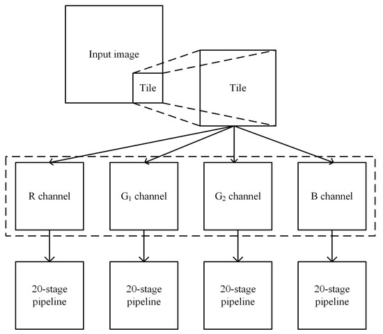
Figure 1.
Tile-based and channel-separated compression method.
The purpose of segmenting the image into tiles is to enhance radiation resistance. When a tile within an image experiences single-bit or multi-bit flips, the image can still be decoded. The independent compression of each color channel within the tiles further enhances radiation resistance. In the event of data corruption, the impact is confined to a single channel within a specific tile, thereby minimizing the overall degradation of image quality. Additionally, compressing each color channel separately preserves the unique characteristics of each channel, allowing the compression method to adapt to various Bayer patterns and different numbers of color channels. This approach ensures the robustness and flexibility of the compression algorithm across different imaging scenarios.
Upon dissection into tiles, each channel is sequentially fed into the compression algorithm for processing. To ensure proper handling of the edges, boundary data is padded to extend the nxn into an (n + 1) × (n + 2) configuration. Taking the 4 × 4 size as an example, the data lying between the red and blue regions in Figure 2 represents the padding. Specifically, the first row is padded with zeros. The subsequent first column is replicated from the second of the preceding row, and the final column mirrors the corresponding row’s first column data from the original channel. The lower right corner of the channel is designated as an irrelevant area and does not participate in the compression.
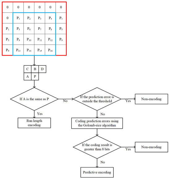
Figure 2.
Overview of the hybrid strategy-based lossless compression algorithm.
Once the channel is prepared and padded, the compression operation is executed in ascending order of indices for each component ‘P’. In addition to the target component that needs to be compressed, contextual elements ‘A’, ‘B’, ‘C’, and ‘D’ are also required. If ‘P’ matches ‘A’, run length encoding is applied to compress the component. In cases of non-matching, a decision between non-encoding and predictive encoding is made based on the prediction error and the bit count of the Golomb–Rice coding (GRC) [19]. If the prediction error exceeds a predefined threshold or if the GRC requires more bits than the storage capacity of the component, the algorithm opts for non-encoding. Otherwise, predictive encoding is used. It is assumed that the components are 8 bits. If the GRC exceeds 8 bits, non-encoding should be selected.
2.1. Run Length Encoding
Run Length Encoding (RLE), a potent lossless compression algorithm, leverages the redundancy prevalent in spatially correlated pixels. The mechanism of RLE entails sequentially scanning an image and transmuting the contiguous runs of identical pixels into a condensed format.
The RLE method deployed in this study extends the conventional definition of a “run”, which we redefine as a series of spatially consecutive components that replicate the value of their antecedent component ‘A’. As shown in Figure 3, the components are part of a channel. The components ‘0xEE 0xAA,’ encapsulated by the orange border, are filled based on predefined rules. The examination commences from left to right within the first row. The initial ‘0xBB’ component’s antecedent ‘A’ is ‘0xAA’, necessitating predictive encoding or non-encoding for its compression. The subsequent two ‘0xBB’ components, having a preceding ‘A’ of ‘0xBB’, are merged into the same run sequence. Subsequent scrutiny progresses in a left to right manner along the second row. The filling strategy facilitates that the antecedent component for the first ‘0xAA’ is not ‘0xBB’ but the fill-inferred ‘0xAA’. Similarly, the following two ‘0xAA’ components, with a preceding ‘A’ of ‘0xAA’, allow the ‘0xAA’ component in the second row to be encoded into the preceding run. This results in a run length of 4, despite ‘0xBB’ and ‘0xAA’ being different values. This augmented “run” definition enhances the compressive capabilities of RLE, enabling a greater quantity of components to be subsumed within the same run sequence. Ultimately, the run length ‘n’ is converted into ‘n − 1’ bits of binary 1’s followed by a single bit of binary 0, culminating in the resultant run length code. In the above example, with a run length of 4, the components ‘0xBB 0xBB 0xAA 0xAA’ would be compressed into 3 bits of binary 1s followed by 1 bit of binary 0. In the event that the run length exceeds the maximum value that can be represented by the bit depth, the run will be interrupted and the maximum value that the bit depth can represent will be output.
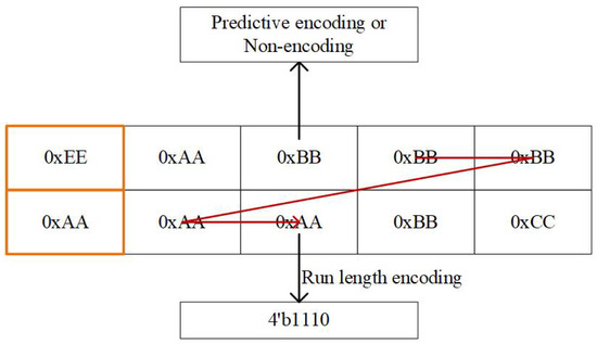
Figure 3.
Example of the RLE method we used.
This methodology amplifies compression efficacy without sacrificing the lossless nature of the output, showcasing a significant improvement over traditional RLE approaches. The extended run concept embodied in our algorithm not only optimizes the encoding length but also simplifies the decoding process.
2.2. Predictive Encoding
The essence of predictive coding lies in context modeling. Context modeling involves capturing the correlation between subpixel ‘P’ and its neighboring subpixels ‘A’, ‘B’, ‘C’, and ‘D’. Initially, context modeling estimates local gradients , , and based on the values of the adjacent pixels, as shown in Equation (1).
As shown in Equation (2), we obtain the quantized gradients , , and by quantizing the local gradients. Here, , as defined in Equation (3), is a piecewise function that maps the range [−255, 255] to [−4, 4].
After obtaining the quantized values, q is calculated using Equation (4), which ranges from [1, 364]. The SIGN represents the sign bit of the first non-zero element among , , and .
The value q is used to address the context arrays N and A, obtaining the context parameters and , as shown in Equation (5).
As shown in Equation (6), a median edge detection is performed on the context to form the predicted value for the current component ‘p’.
After obtaining the Golomb encoding parameter k, calculate the remaining two encoding parameters and using Equation (10). Once parameters are determined, encode using GRC to obtain the predicted encoding result.
2.3. Non-Encoding
In the intricate field of image compression, the strategic omission of encoding under specific conditions has emerged as a pivotal technique to enhance compression ratios while concurrently expediting the encoding and decoding processes. The judicious application of non-encoding, in scenarios where predictive encoding breaches specified bit thresholds, necessitates a decision within the compression algorithm.
Non-encoding is primarily applied in two situations. The first occurs when the bit count required by Golomb–Rice coding exceeds the available storage capacity, making the encoded length larger than that of the non-encoded representation. In such cases, encoding is bypassed to conserve storage space, although arrays A and N must still be updated. The continuous update of these arrays plays a vital role in refining the predictive process and guiding the algorithm’s parameters toward an optimal balance.
The second situation arises when the absolute value of the prediction error surpasses a predefined threshold, set to 64 in this study. Under these conditions, encoding the prediction error would require more bits than the available storage capacity, so the process is terminated in favor of non-encoding. In this case, updates to arrays A and N are unnecessary. This approach reduces computational overhead and improves the compression ratio.
This non-encoding strategy ensures that the worst-case scenario is capped to the size of the original data. This constraint is not merely a safeguard but also a facilitator for augmenting compression capability and accelerating the compression-decompression cycle. By integrating non-encoding strategies, the compression algorithm is fortified against inefficiencies when predictive encoding fails, thus maintaining high performance.
3. Implementation
The compression module designed in this paper adopts pipeline architecture, and the architecture is shown in Figure 4. The whole architecture is divided into the 20 stages of the pipeline. The main functions of each stage of the pipeline are introduced below.
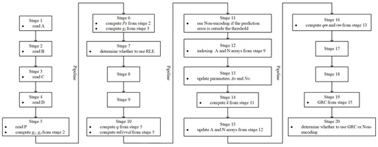
Figure 4.
Twenty-stage pipeline for the hybrid strategy-based lossless compression algorithm.
Stage 1 to Stage 4: Contextual elements ‘A’, ‘B’, ‘C’, and ‘D’ are read.
Stage 5: The component ‘P’ is read. Following the completion of stage 3 and the acquisition of ‘C’, the parameters and begin to be calculated, according to Equation (1).
Stage 6: After stage 3 completes, parameter starts to be calculated, according to Equation (6). Once stage 4 completes, the calculation of parameter begins, according to Equation (1).
Stage 7: ‘A’ and ‘P’ are checked for equality. If they are equal, the pipeline terminates and RLE is used. If they are not equal, the pipeline continues execution.
Stage 10: Following the completion of stage 6, parameters q and begin to be calculated, according to Equations (2), (4), (7) and (8).
Stage 11: is checked against a threshold. If it exceeds the threshold, the pipeline terminates and non-encoding is used. If it does not exceed the threshold, the pipeline continues execution.
Stage 12: Following the completion of stage 10, q is used to index arrays A and N to retrieve parameters and . Arrays A and N are stored in a block RAM (BRAM). To improve the timing of the BRAM output interface, the output interface register is enabled, requiring two clock cycles to index this BRAM.
Stage 13: The updated values for parameters and are calculated based on predefined rules, according to Equations (11) and (12).
Stage 14: Following the completion of stage 12 and the stabilization of BRAM output, the calculation of parameter k begins, according to Equation (9).
Stage 15: Following the completion of stage 13, q is used as the index for arrays A and N, and the updated values of and are written into the corresponding arrays.
Stage 16: Following the completion of stage 13, the calculation of parameters and begins, according to Equation (9).
Stage 19: Following the completion of stage 16, is coded using GRC.
Stage 20: After obtaining the GRC coding of , if the coding exceeds the storage capacity of component ‘P’, non-encoding is used. Otherwise, predictive encoding is used, with the GRC coding as the result of predictive encoding.
To increase the clock frequency, the calculations of , , , q, , k, , , and GRC within the pipeline are designed as multi-cycle operations. These multi-cycle operations introduce structural hazards. The updating and reading of arrays are discrete processes, with updates completing in stage 15 and reading completing in stage 12. If the same index is used, reading the arrays before updating will cause flow dependence data hazards. The pipeline has three potential termination points: stage 7, stage 11, and stage 20. If the current pipeline terminates at stage 11 and the subsequent pipeline terminates at stage 7, it leads to the latter pipeline finishing earlier than the former. This discrepancy can result in the termination order being inconsistent with initiation order, potentially disrupting the orderly flow of data. To manage the above challenges, three methods are proposed.
The 20-stage pipeline architecture is designed to enhance operating frequency, but it also introduces significant complexity and synchronization challenges. The main difficulty arises from the control overhead required to manage three distinct termination points, located at stages 7, 11, and 20, together with the corresponding data flow control. Each termination point must be supported by different control logic and data handling mechanisms, which increases the overall complexity of the control system. Synchronization issues appear because the reorder buffer must accommodate variable-latency outputs from multiple termination points, while the key-value register system must preserve consistency across all pipeline stages. At the same time, the bypass mechanism is required to route data correctly according to the specific termination path.
To address these challenges, a centralized control unit is employed to monitor the state of each pipeline instance and to coordinate the movement of data. The control overhead is further reduced through the use of dedicated control signals for each termination path and by implementing simplified state machines for pipeline management. As a result, the trade-off between deeper pipelining and greater control complexity is carefully balanced, ensuring that the performance gains obtained from higher operating frequencies outweigh the additional control cost.
The 20-stage pipeline was not chosen arbitrarily but was derived through stage-level timing decomposition. Complex arithmetic operations, memory accesses, control decisions, and entropy coding were each assigned to logically distinct stages in order to minimize the logic depth per stage and the corresponding clock period. Several operations within the pipeline are inherently multi-cycle, meaning they cannot be completed within a single clock cycle. For example, in stage 10, the calculation of the parameters q and is initiated as early as stage 5, but under high-frequency timing constraints, five cycles are required to produce the results. Stages 8 and 9 were therefore inserted to satisfy the required five-cycle delay, and the same rationale applies to stages 17 and 18. In addition, the computational units within the pipeline are replicated as needed so that new operations can be admitted on every cycle, ensuring continuous execution. Further details regarding this aspect are provided in the section on structural hazards.
3.1. Structural Hazards
Structural hazards in a pipeline occur when resources are insufficient to support all the concurrent operations required in a given clock cycle. These hazards arise due to conflicts over the usage of the same resources. Certain operation, such as the computation of G2 in stage 5, require two clock cycles to complete, necessitating the calculation to commence as early as the end of stage 3. When adjacent pipeline instances need to compute G2, a conflict arises because the subsequent pipeline cannot proceed until the current pipeline releases the occupied resource.
To address this issue, dual instances of the computing unit for G2 are instantiated. This ensures that subsequent operations can proceed unhindered by utilizing the alternate computing unit. The replication of computing units, scaled to match their computation cycles ‘n’, is an effective resolution of structural hazards. Specific measures to address the remaining structural hazards within the pipeline are detailed in Table 1.

Table 1.
Number of replications of computer units.
3.2. Data Hazards
Flow dependence data hazards, also known as read-after-write (RAW) hazards, occur when a subsequent operation attempts to read data before the previous write operation has completed. Consider a pipeline instance that uses the index to access arrays A and N at the end of stage 10. This instance updates the parameters and based on at the end of stage 15. It is only after the completion of stage 15 that other pipeline instances can safely access A[] and N[]. If the subsequent pipeline instances attempt to access A[] and N[] before the update is complete, flow dependence data hazards will occur. These hazards arise because the subsequent instances might read outdated values from arrays A and N.
To circumvent these hazards, key-value registers and bypass are introduced, as illustrated in Figure 5. The keys of these registers correspond to the BRAM index addresses, while the value entries hold the updated parameters and . Key-value registers are added for stages 12, 13, 14, and 15. Specifically, the value for stage 12 is bypassed directly from the computation results of stage 13. The comparison and selection processes are completed within two pipeline stages, with their operations described by Equations (13) and (14), respectively. These equations describe the operation of the Comparison Q and Selection Q modules illustrated in Figure 5. The Comparison Q module, which follows Equation (13), receives five inputs , , , , and . Its function is to identify the first matching parameter among the inputs and to generate a one-hot code that marks the position of the match. The Selection Q module, which follows Equation (14), receives inputs , , , , together with the one-hot code C. Based on this code, the corresponding parameter is selected as the output. In stage 11, q is compared with four keys, generating a one-hot code used for selection. Each clock cycle, q is written into the key register of the next stage. In stage 12, the code generated in the previous stage is used to decide whether to read and from BRAM or use the values from other stages. Specifically, whether to use the stage 12 value is determined in stage 13. When one-hot code[1] is 1, the input for updating parameters and uses the output and from the same stage. When one-hot code[1] is 0, the stage 12 value is not used, and the output a and n from stage 12 are used instead. Each clock cycle, the stage 12 value is sequentially written into the value register of the next stage. This mechanism ensures that the most recent data is used.
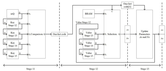
Figure 5.
Architecture for solving data hazards.
3.3. Reorder Buffer
To avert such blocking, a reorder buffer is implemented, depicted in Figure 6, allowing for the resequencing of out-of-order pipeline outputs. The worst-case scenario is characterized by the first component concluding at stage 20 while subsequent components complete at stage 7, with 12 subsequent component results being outputted before the first. To account for this, the reorder buffer is sized beyond 12, set to 16 in our design, to accommodate any potential out-of-order outcomes. The reorder buffer utilizes cyclical counters on both the read and write sides for indexing, with a one-bit valid flag indicating the buffer’s status, initialized to 0. The counters are five bits wide, with the lower four bits, initially set to 0, used for indexing and the upper bit, initially set to one, serving as the valid flag. On the write side, after data insertion using the lower four bits as the address, the fifth bit updates the valid flag. On the read side, when the valid flag matches the counter’s highest bit, the data is ready for retrieval. The read side uses the lower four bits of the counter to index the reorder buffer. In the example illustrated in Figure 7, the write side has already inserted data into addresses 1 and 2 of the reorder buffer. The read side is waiting for data at address 0. Once the data at address 0 becomes valid, the read side will sequentially read the data from addresses 0, 1, and 2. Thus, data written out of order to addresses 1, 2, and 0 will be read in the correct order as 0, 1, and 2 by the read side.
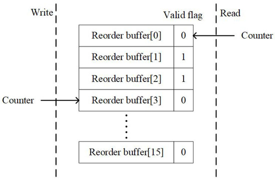
Figure 6.
Example of reorder buffer.
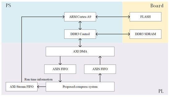
Figure 7.
Experimental platform for public datasets.
The reordering procedure introduces additional latency that must be carefully controlled in order to preserve the benefits of pipelining. The extent of this latency is determined by the degree of out-of-order execution and the level of reorder buffer utilization. In the worst case, when the first component requires 20 stages while subsequent components require only 7 stages, the reorder buffer must wait for the longest operation to complete before the first result can be released. This situation produces a latency penalty of up to 13 clock cycles, although the penalty is distributed across the processing of an entire tile. Because of the continuous operation of the pipeline, overall throughput remains high despite this delay.
The reorder buffer has been designed to minimize the effect of latency through careful architectural choices. The buffer size of 16 entries was selected to balance latency with resource usage. A cyclical counter system has been introduced to enable efficient buffer management without the need for complex address calculations, while a valid-flag mechanism allows immediate output as soon as data becomes available. The architecture further ensures that output order is maintained without additional synchronization overhead, since the read and write pointers are managed independently. As a result, the latency penalty is considered acceptable in view of the significant throughput gains offered by the pipeline, and deterministic output ordering is preserved to guarantee accurate image reconstruction.
The depth of the reorder buffer is determined by the timing at which data exits the pipeline. In the pipeline design under consideration, the worst-case scenario occurs when the first component completes at stage 20, while subsequent components finish at stage 7. In this interval, up to 12 components may exit the pipeline out of order. The capacity of the reorder buffer is therefore specified based on the maximum number of out-of-order data items in this worst-case scenario. For larger data volumes, the depth of the reorder buffer remains unaffected. As the pipeline depth increases further, the number of out-of-order data items in the worst case may also increase, necessitating a corresponding increase in the reorder buffer capacity. Deeper pipelines require larger buffers, which increases memory demand and may potentially impact timing closure. The circular counter system can be effectively scaled with the buffer size, as the counter width can be increased to accommodate a larger buffer without requiring significant architectural modifications. However, larger buffers introduce additional complexity in managing valid flags and coordinating read/write pointers.
4. Validation and Analysis
4.1. Experimental Settings
The compression system was implemented on the Xilinx ZC706 evaluation board [20]. The FPGA used is the Zynq-7000 XC7Z045-2FFG900C (Xilinx, Inc., San Jose, CA, USA) SoC [21], which features two ARM Cortex-A9 MPCore processors (Xilinx, Inc., San Jose, CA, USA), 218,600 LUTs, 437,200 FFs, and 19.16 Mb of BRAM. Experiments were conducted using both public datasets and bayer pattern spaceborne camera. The experimental platforms used are described as follows:
- The experimental platform used to validate the system with public datasets is illustrated in Figure 7. Initially, the dataset is written into the FLASH. The ARM processor in the Processing System (PS) initializes the DDR3 controller to transfer data from FLASH to DDR3 SDRAM. Once the data transfer is complete, the ARM processor again controls the DDR3 controller, sending data from DDR3 SDRAM to the compression system via AXI DMA for compression operations. The ARM processor sends one tile of data to the compression system at a time. Simultaneously, it controls the AXI DMA to forward the compressed data back to DDR3 SDRAM. If the compression system waits for a period without receiving new data, it concludes the compression process and sends an interrupt to the ARM processor via AXI-Stream FIFO, along with information on the runtime. This information is used to calculate the compression efficiency of the system. After compression is complete, the ARM processor reads the compressed data from DDR3 SDRAM and stores it in FLASH for further compression rate calculations.
- The experimental platform used to validate the system with a bayer pattern spaceborne camera is illustrated in Figure 8. Initially, the camera sends photos to the FPGA through an external connector. Upon receiving the data, the FPGA buffers it in DDR3 SDRAM. Once enough data is buffered to extract a tile, the photo is sent to the compression system tile by tile. After the compression system completes the compression, the compressed data is written back to DDR3 SDRAM. When DDR3 SDRAM has available bandwidth, the compressed data is read out and written into FLASH via the FLASH controller. When the first tile of a photo is read from DDR3 SDRAM, the system writes a start timestamp into FLASH. Following the start timestamp, the compressed data for the entire image is stored. After writing the compressed data for the last tile of the photo into DDR3 SDRAM, an end timestamp is written. Once the start timestamp, compressed data, and end timestamp are sequentially written into FLASH, the time taken by the compression system can be calculated by subtracting the start timestamp from the end timestamp.
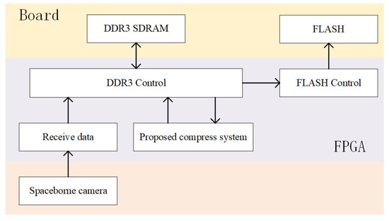 Figure 8. Experimental platform with a Bayer pattern spaceborne camera.
The proposed system was evaluated on six image datasets:
- ImageNet64 [22]: The ImageNet64 dataset is a variant of the widely recognized ImageNet dataset, specifically downsampled to a resolution of 64 × 64 pixels, consisting of 50,000 images.
- DIV2K [23]: The DIV2K dataset contains 100 high-resolution images, featuring diverse and 2K content sourced from various real-world scenes.
- CLIC.p [24]: The CLIC professional dataset features 41 high-quality color images taken by professional photographers, primarily in 2K resolution, used for benchmarking image compression and quality enhancement algorithms.
- CLIC.m [24]: The CLIC mobile dataset includes 612K high-resolution images captured using mobile devices. While most images in the CLIC.m dataset are in 2K resolution, some are smaller in size.
- Kodak [25]: The Kodak dataset consists of 24 uncompressed color images at a resolution of 768 × 512 and is widely used for evaluating image compression methods.
- Custom: The custom test image set, consisting of 10 images of various types with 8-bit depth and multiple sizes, was used to validate and analyze the performance of the proposed system.
The rationale for dataset selection is to cover a broad spectrum of image characteristics. The datasets span from low to high resolutions and include both professional and mobile imagery, as well as established benchmarks. They contain diverse textures, smooth regions, and edges, which affect predictive coding and run-length encoding in different ways. ImageNet64 is used to examine behavior under low resolution with high content diversity. DIV2K and CLIC.p capture the fine details of professional high-resolution images. CLIC.m reflects the statistical properties and noise patterns of mobile imagery. Kodak serves as a long-standing benchmark that enables comparison with prior lossless codecs. A custom dataset is included to address Bayer-like patterns and operational dimensions. This combination provides a representative basis for evaluating Bayer-oriented lossless compression under different statistical conditions and scales. It also aligns with the requirements of spaceborne scenarios, which range from smooth terrains to high-contrast structures.
The following criteria are commonly used to evaluate the hardware compression performance:
- Compression ratio: The compression ratio is defined as the ratio of the information amount of the source image to the information amount of the compressed image, as shown in Equation (15). Here, c represents the compression ratio, n1 denotes the information amount of the source image, and n2 signifies the information amount of the compressed image. In lossless compression, a higher compression ratio indicates better compression performance.
- Clock frequency: Clock frequency refers to the operating frequency of the timing logic within the FPGA and is closely related to the computational capacity of the FPGA. A higher clock frequency indicates that the hardware architecture operates at a faster speed.
- Throughput: In compression, throughput refers to the amount of data compressed per unit of time, typically measured in pixel per second (pixel/s) or subpixel per second (subpixel/s). Throughput serves as an indicator of the performance and efficiency of a compression system. Generally, higher throughput signifies faster compression speeds.
- Resource utilization: Lookup Table (LUT) resources and slice resources are two types of logic resources in an FPGA, each serving different functions. LUTs can store truth tables to implement combinational logic or distributed memory. Slices, composed of multiple LUTs and flip-flops (FFs), can perform sequential logic, arithmetic operations, data selectors, and more. Generally, lower resource utilization indicates lower power consumption and greater robustness in resource-constrained environments.
4.2. Compression Ratio of Proposed System
The lossless image compression ratio of the proposed system was evaluated using tile sizes of 4 × 4, 8 × 8, 16 × 16, and the full image. To objectively assess the compression efficiency of the proposed system and facilitate comparison with other methods, it was applied to publicly available ARGB and RGB datasets. It is important to note that, although the system is specifically designed for Bayer pattern images, it is also capable of compressing ARGB or RGB images. We compare with eight traditional lossless image codecs, including PNG [26], JPEG-LS [3], CALIC [27], JPEG2000 [28], WebP [29] and BPG [30], and two recent learning-based lossless image compression methods, including L3C [13] and RC [31]. The results are detailed in Table 2. Table 2 is primarily used for cross-comparing the compression results of different methods. Regarding the impact of different image patterns on compression, further discussion and analysis will be provided in subsequent articles.
Table 2.
Comparisons with other method using compression ratio metric.
It should be specifically noted that when tile sizes of 32 × 32 or larger are used, the compression ratio remains essentially the same as that obtained with 16 × 16 tiles. For this reason, only the results for 16 × 16 tiles and full-frame compression are reported in the table. The proposed encoding system has been demonstrated to achieve optimal compression performance across a range of datasets, including ImageNet64, CLIC.p, CLIC.m, and Kodak, under full-image compression conditions. The system demonstrates superior compression on the ImageNet64 validation dataset with WebP and BPG, and outperforms JPEG-LS. When the tile size is set to 16 × 16, the system achieves the second-best ranking on the ImageNet64 and CLIC.p datasets, while demonstrating the best performance on the remaining datasets. However, a notable decline in compression efficiency is observed when the tile size is set to 4 × 4. These results indicate that our compression system delivers excellent lossless image compression performance for both full-image and 16 × 16 tile sizes, making it highly applicable to various domains and image modalities.
4.3. Performance of Proposed System
The performance of the proposed hardware implementation is compared with seven other designs, as shown in Table 3. In the case that the necessary resources are available, simply replicating the system can facilitate parallel compression. In order to facilitate an objective comparison of the relative merits of each method, the table only includes scenarios where each system operates independently. The comparison considered throughput, logic overhead, memory usage, and hardware platform. To intuitively analyze the impact of different image patterns and tile sizes on compression results, a custom test set was used to test the compression system with tile sizes of 4 × 4, 8 × 8, 16 × 16, and the full image. For a more equitable cross-comparison, our design has been implemented across multiple platforms. In designs developed after 2018, devices from the Virtex-6, Virtex-7, and Zynq-7000 (Xilinx, Inc., San Jose, CA, USA) families have been primarily adopted by other research efforts. Therefore, our design has also been implemented on devices belonging to these three families to enable a more equitable cross-comparison and eliminate the influence of device variations.
Table 3.
Comparisons with other implementations.
- Throughput: The PEP architecture [32] is currently the most performant hardware implementation of the JPEG-LS algorithms, without considering software–hardware co-design and multi-core parallel processing. This method implemented the proposed architecture on the XILINX Virtex-6 FPGA (xc6vcx75t-1ff484). For a fair comparison, our system was also implemented on the same FPGA part. The PEP architecture employs a six-stage pipeline operation. Within this pipeline, the critical data path of the PEP architecture uses a two-stage pipeline for calculating prediction errors and updating context parameters. Additionally, the context conflict detector and the proposed equivalent simplified reconstruction scheme further shorten the critical data path. For the PEP architecture, the critical data path delay is 19.35 ns, and the maximum throughput is 51.684 Mpixel/s. In our proposed architecture, a 20-stage pipeline was used, which adds 14 more stages compared to the PEP architecture. Specifically, a 10-stage pipeline is used from the prediction error calculation to the context parameter update, significantly reducing the critical data path. Furthermore, the read and update of the context parameters were refined into a five-stage pipeline. Considering the large data path delay caused by BRAM read and write operations, an additional register was added on both the read and write sides of the BRAM to reduce this delay. This extends the read/write operation from occupying a single pipeline stage to two pipeline stages. Additionally, the operations of BRAM reading, context parameter updating, and BRAM writing were separated, extending the single pipeline stage in the PEP architecture to five pipeline stages. Consequently, the delay of the critical path was optimized to 3.33 ns (300 MHz), and the maximum throughput increased to 296.92 Mpixel/s. It is evident that the proposed architecture achieved more than a 3× throughput speedup compared to the PEP architecture.
- Memory usage: Generally, the pipeline processes images according to the tile scanning order, thereby minimizing memory consumption. Three main processes require memory units: the data buffer, the tile buffer, and the parameter array. The data buffer, primarily an FIFO, is used to cache data after being read from DDR and before being written back. The tile buffer, primarily BRAM, is used to cache a complete tile after the image has been divided into tiles and before being fed into the compression algorithm. The parameter array, also primarily BRAM, stores context parameters. The depth of the data buffer is determined by the data volume that can be transmitted in a single burst operation from DDR, and it is not influenced by the pipeline architecture. The tile buffer size is determined by the maximum tile size the system can support. The depth of the BRAM for context parameters a and n is fixed at 365, with the width determined by the bit depth. In our proposed architecture, the maximum supported tile size is 16 × 16 with a bit depth of eight bits, and it supports up to four channels. Consequently, each tile buffer has a size of 17 × 18 with a width of eight bits. Specifically, the tile buffer stores a complete expanded tile, where the original tile size is nxn, and the expanded size is (n + 1) × (n + 2). We adopted a subpixel approach, with the number of tile buffers determined by the number of supported pixel channels. Thus, our system employs four tile buffers, each with a width of eight bits and a size of 306. The BRAM depth for storing context parameters is 365, with the widths of parameters and being 16 bits and 8 bits, respectively, for an 8-bit subpixel.
- Effect of the image pattern on compression ratio: The smoothness of an image significantly affects the compression performance of the proposed algorithm. Images with high smoothness exhibit small variations in the grayscale values of adjacent pixels, resulting in mostly small or zero prediction errors that can be represented with fewer bits, thereby enhancing both compression ratio and speed. Conversely, images with low smoothness show large variations in grayscale values between adjacent pixels, leading to larger and less frequent zero or near-zero prediction errors, which require more bits to represent, thereby reducing both compression ratio and speed. For instance, due to the high smoothness of sample 1, many pixels fall into flat regions, allowing the use of run-length encoding for a majority of the pixels, resulting in efficient compression, as show in Table 4. In contrast, sample 9 has lower smoothness, with fewer pixels falling into flat regions, meaning fewer pixels can be encoded using run-length encoding, resulting in a lower compression ratio. In the context of spaceborne camera images, which are typically smooth, this algorithm is expected to achieve favorable compression results.
Table 4. Compression results of custom dateset.
- Effect of the tile size on compression ratio: To investigate how to determine the appropriate tile size, the compression ratio was tested with image tiles of various sizes. The compression ratio results for each tile size are presented in Table 4. It can be observed that as the tile size increases, the compression ratio moderately increases. Compared to the full-size image, the compression ratio for a tile size of 16 × 16 shows a slight reduction, with an summary loss of approximately 0.005. Additionally, the compression ratios for smaller tile sizes indicate that their compression ratio values are relatively close to each other. However, larger tile sizes lead to increased memory usage and longer compression delays. Therefore, the block size cannot be set too large. Consequently, a 16 × 16 tile size is preferred as the maximum block size for our implementation. Tile size selection significantly impacts both error resilience and compression efficiency, creating a fundamental trade-off that must be carefully balanced. Larger tiles provide better compression efficiency due to increased context availability and reduced boundary effects, but they also increase the impact of single-bit errors. When a bit flip occurs in a large tile, the error can propagate throughout the entire tile, affecting up to 256 pixels in a 16 × 16 tile. Conversely, smaller tiles provide excellent error isolation, limiting error propagation to at most 16 pixels, but suffer from reduced compression efficiency due to limited context and increased boundary overhead. The experimental results demonstrate this trade-off clearly: 16 × 16 tiles achieve compression ratios close to full-image processing, within 0.005, while 4 × 4 tiles show significantly reduced compression ratios, approximately 15–20% lower. The error resilience analysis reveals that larger tiles are more susceptible to radiation-induced bit flips, as a single error can corrupt a larger portion of the image. However, the tile-based approach still provides substantial protection compared to full-image processing, where a single error could potentially corrupt the entire image. The 8 × 8 tile size represents a reasonable compromise, offering moderate compression efficiency while maintaining good error isolation. For spaceborne applications where radiation tolerance is critical, the choice between tile sizes should be based on the specific mission requirements, with smaller tiles preferred for high-radiation environments and larger tiles for applications where compression efficiency is paramount.
- Computational complexity and runtime analysis: An analysis of computational complexity and execution time demonstrates the efficiency of the proposed encoder. For each component, the operations required by the design consist of constant-time neighborhood access, fixed-cost gradient quantization combined with median-edge prediction, addressing and updating of context arrays, and Golomb-Rice coding of the prediction error. Each of these operations is characterized by complexity with a small constant factor, and they are executed within a 20-stage pipeline equipped with multiple functional units. In contrast, conventional JPEG-LS software (version 2.2) implementations exhibit similar asymptotic complexity but lack the advantages of deep hardware pipelining, particularly at high operating frequencies. Experimental evaluation confirms the benefits of the hardware implementation. A processing speed of up to 346.41 MPixel/s has been achieved, representing at least a threefold improvement over previous JPEG-LS accelerators implemented on comparable chips. The runtime for a 2K frame is reduced to the microsecond level, whereas software implementations of JPEG-LS executed on embedded CPUs or GPUs are slower by several orders of magnitude and consume significantly more energy. The pipeline structure further ensures that the latency per component remains constant, which stabilizes performance across varying workloads. These results highlight the ability of the architecture to combine low computational complexity with high throughput and energy efficiency, making it particularly well suited for real-time spaceborne imaging applications.
4.4. Performance of Proposed System on Bayer Pattern Spaceborne Camera
In space, bit flips caused by radiation can lead to error propagation effects, which are inherent to compression systems. Error propagation occurs when single or multiple bit errors in the bitstream spread, resulting in reconstruction errors for consecutive pixels. In our tile-by-tile, channel-separated compression mode, each tile is independently encoded, naturally limiting reconstruction errors within the tile and preventing error propagation to the rest of the image. We investigated the error propagation effects for different tile sizes through simulation experiment. The results demonstrated that, under three different tile sizes, errors were not propagated. Instead, they were confined within a single tile and did not affect the other tiles.
Error propagation in the deep 20-stage pipeline presents unique challenges that must be carefully mitigated. A single bit flip within the pipeline can influence multiple stages, especially when it occurs in critical data paths such as context parameter updates or prediction calculations. The severity of such an error depends largely on its location. When errors arise in the early stages, context reading and initial calculations are affected. Errors in the middle stages tend to disrupt context parameter updates and prediction error calculations, while those occurring in the later stages primarily influence the final encoding process.
To address these risks, a combination of mitigation techniques has been integrated into the design. Parity checking is applied at critical stages to detect potential bit flips, and redundant computation units are employed for essential operations to enable error detection and correction. Context parameters are validated before updates to prevent corruption of context arrays, and mechanisms for graceful degradation are introduced to allow continued system operation even in the presence of detected faults. Additional protection is offered by the tile-based approach, since errors are confined to individual tiles rather than spreading across the entire image. Moreover, the key-value register system incorporates error detection features that flag corrupted context parameters before they are used in subsequent calculations.
5. Conclusions
This paper proposes a compression algorithm similar to JPEG-LS and presents its high-performance hardware implementation. A tile-based and channel-separated compression approach is adopted to prevent and limit potential error propagation effects within individual tile, thereby enhancing radiation resistance. The algorithm is implemented using a 20-stage pipeline. Within the pipeline, computation unit duplication, key-value registers, bypass mechanism and reorder architecture are employed to resolve structural hazards, data hazards, and out-of-order data issues, respectively. The proposed architecture is implemented on the Zynq-7000 XC7Z045-2FFG900C SoC (AMD, San Jose, CA, USA), achieving a maximum throughput of 346.41 MPixel/s. It is the fastest hardware architecture reported in the literature that implements lossless compression for JPEG-LS or similar algorithms. Our architecture is fully realizable with basic logic resources and can be further mapped onto other FPGA or ASIC technologies. Future work may include further optimizing the timing paths for the computation and updating of context parameters to increase the operating frequency of the hardware implementation.
The proposed design demonstrates significant potential for scaling on parallel architectures and multi-core processors. The tile-based processing approach naturally enables parallel execution, as each tile can be processed independently by separate processing units. However, the current implementation faces certain limitations in pipeline efficiency that could impact parallel scalability. The primary bottleneck lies in the dependency on context parameter updates (arrays A and N) which require sequential access patterns. While the key-value registers and bypass mechanism mitigate some data hazards, the fundamental sequential nature of context modeling limits the degree of parallelization achievable. Additionally, the reorder architecture introduces synchronization overhead that becomes more pronounced as the number of parallel processing units increases. To fully leverage multi-core architectures, future implementations would benefit from context parameter partitioning strategies and more sophisticated load balancing mechanisms.
With respect to scalability for larger datasets and ultra-high-resolution images in future space missions, the proposed system is considered highly advantageous. A tile-based approach is inherently scalable, since memory requirements increase linearly with tile size rather than with overall image size. For 8K or higher resolution images, the system can process data in a streaming manner without the need to load the entire image into memory at once. In addition, the current pipeline depth is fixed. Images of different resolutions are divided into tiles for processing, and the latency remains unchanged. The size of the reordering buffer is also not required to be expanded to accommodate larger tile sizes. Instead, the buffer size depends only on the pipeline depth and the earliest exit point of data from the pipeline, neither of which is affected by image resolution.
Future work will focus on several directions that aim to enhance both performance and adaptability. Adaptive adjustment of tile size is expected to balance compression ratio, radiation robustness, and latency under varying scene statistics. Bayesian or lightweight learning-based priors may be incorporated to improve context modeling without compromising FPGA frequency. Multi-core or NoC deployment is envisioned, where partitioned context arrays and coordinated scheduling enable linear scalability with the number of cores. On-orbit upgrades may be supported through partial reconfiguration, allowing thresholds such as hysteresis margins to be adjusted in response to radiation conditions and imaging environments. The framework may also be extended to multispectral and hyperspectral mosaics by generalizing the channel-separated dataflow and context design.
Author Contributions
Conceptualization, X.L.; Software, X.L.; Validation, X.L.; Formal analysis, X.L.; Investigation, X.L. and L.Z.; Resources, L.Z.; Data curation, X.L.; Writing—original draft, X.L.; Writing—review and editing, X.L.; Visualization, Y.Z.; Supervision, L.Z.; Project administration, Y.Z. All authors have read and agreed to the published version of the manuscript.
Funding
This research received no external funding.
Data Availability Statement
The raw data supporting the conclusions of this article will be made available by the authors on request.
Conflicts of Interest
The authors declare no conflicts of interest.
References
- Takhtkeshha, N.; Mandlburger, G.; Remondino, F.; Hyyppä, J. Multispectral light detection and ranging technology and applications: A review. Sensors 2024, 24, 1669. [Google Scholar] [CrossRef] [PubMed]
- Ye, S.; Yu, X.; Gan, G. Design and implementation of spaceborne multispectral camera imaging system. Acta Opt. Sin. 2023, 43, 2411001. [Google Scholar]
- Weinberger, M.; Seroussi, G.; Sapiro, G. The LOCO-I lossless image compression algorithm: Principles and standardization into JPEG-LS. IEEE Trans. Image Process. 2000, 9, 1309–1324. [Google Scholar] [CrossRef] [PubMed]
- Rane, S.; Sapiro, G. Evaluation of JPEG-LS, the new lossless and controlled-lossy still image compression standard, for compression of high-resolution elevation data. IEEE Trans. Geosci. Remote Sens. 2001, 39, 2298–2306. [Google Scholar] [CrossRef]
- Sun, X.; Chen, Z.; Wang, L.; He, C. A lossless image compression and encryption algorithm combining JPEG-LS, neural network and hyperchaotic system. Nonlinear Dyn. 2023, 111, 15445–15475. [Google Scholar] [CrossRef]
- Miaou, S.G.; Ke, F.S.; Chen, S.C. A Lossless Compression Method for Medical Image Sequences Using JPEG-LS and Interframe Coding. IEEE Trans. Inf. Technol. Biomed. 2009, 13, 818–821. [Google Scholar] [CrossRef] [PubMed]
- Wang, X.; Gong, L.; Wang, C.; Li, X.; Zhou, X. UH-JLS: A Parallel Ultra-High Throughput JPEG-LS Encoding Architecture for Lossless Image Compression. In Proceedings of the 2021 IEEE 39th International Conference on Computer Design (ICCD), Storrs, CT, USA, 24–27 October 2021; pp. 335–343. [Google Scholar] [CrossRef]
- Liu, F.; Chen, X.; Liao, Z.; Yang, C. Adaptive Pipeline Hardware Architecture Design and Implementation for Image Lossless Compression/Decompression Based on JPEG-LS. IEEE Access 2024, 12, 5393–5403. [Google Scholar] [CrossRef]
- Ferretti, M.; Boffadossi, M. A parallel pipelined implementation of LOCO-I for JPEG-LS. In Proceedings of the 17th International Conference on Pattern Recognition, 2004, ICPR 2004, Cambridge, UK, 26–26 August 2004; Volume 1, pp. 769–772. [Google Scholar] [CrossRef]
- Kagawa, H.; Ito, Y.; Nakano, K. Throughput-Optimal Hardware Implementation of LZW Decompression on the FPGA. In Proceedings of the 2019 Seventh International Symposium on Computing and Networking Workshops (CANDARW), Nagasaki, Japan, 26–29 November 2019; pp. 78–83. [Google Scholar] [CrossRef]
- Tong, L.Y.; Lin, J.B.; Deng, Y.Y.; Ji, K.F.; Hou, J.F.; Wang, Q.; Yang, X. Lossless Compression Method for the Magnetic and Helioseismic Imager (MHI) Payload. Res. Astron. Astrophys. 2024, 24, 045019. [Google Scholar] [CrossRef]
- Bai, Y.; Liu, X.; Wang, K.; Ji, X.; Wu, X.; Gao, W. Deep Lossy Plus Residual Coding for Lossless and Near-Lossless Image Compression. IEEE Trans. Pattern Anal. Mach. Intell. 2024, 46, 3577–3594. [Google Scholar] [CrossRef] [PubMed]
- Mentzer, F.; Agustsson, E.; Tschannen, M.; Timofte, R.; Van Gool, L. Practical Full Resolution Learned Lossless Image Compression. In Proceedings of the 2019 IEEE/CVF Conference on Computer Vision and Pattern Recognition (CVPR), Long Beach, CA, USA, 15–20 June 2019; pp. 10621–10630. [Google Scholar] [CrossRef]
- Zhang, S.; Zhang, C.; Kang, N.; Li, Z. ivpf: Numerical invertible volume preserving flow for efficient lossless compression. In Proceedings of the IEEE/CVF Conference on Computer Vision and Pattern Recognition, Nashville, TN, USA, 20–25 June 2021; pp. 620–629. [Google Scholar]
- Hong, D.; Li, C.; Yokoya, N.; Zhang, B.; Jia, X.; Plaza, A.; Gamba, P.; Benediktsson, J.A.; Chanussot, J. Hyperspectral Imaging. arXiv 2025, arXiv:2508.08107. [Google Scholar] [PubMed]
- Zeng, J.; Jeong, J.; Jung, C. Persistent processor architecture. In Proceedings of the 56th Annual IEEE/ACM International Symposium on Microarchitecture, Toronto, ON, Canada, 28 October–1 November 2023; pp. 1075–1091. [Google Scholar]
- Chaturvedi, I.; Godala, B.R.; Wu, Y.; Xu, Z.; Iliakis, K.; Eleftherakis, P.E.; Xydis, S.; Soudris, D.; Sorensen, T.; Campanoni, S.; et al. GhOST: A GPU out-of-order scheduling technique for stall reduction. In Proceedings of the 2024 ACM/IEEE 51st Annual International Symposium on Computer Architecture (ISCA), Buenos Aires, Argentina, 29 June–3 July 2024; pp. 1–16. [Google Scholar]
- Zhang, L.; Zhang, P.; Song, C.; Zhang, L. A Simplified Predictor With Adjustable Compression Ratio Based on CCSDS 123.0-B-2. IEEE Geosci. Remote Sens. Lett. 2025, 22, 5502005. [Google Scholar] [CrossRef]
- Golomb, S. Run-length encodings (Corresp.). IEEE Trans. Inf. Theory 1966, 12, 399–401. [Google Scholar] [CrossRef]
- Xilinx. ZC706 Evaluation Board for the Zynq-7000 XC7Z045 SoC User Guide (UG954), 2.3 ed.; Xilinx: San Jose, CA, USA, 2022. [Google Scholar]
- Xilinx. Zynq-7000 SoC Data Sheet: Overview (DS190), 2.1 ed.; Xilinx: San Jose, CA, USA, 2021. [Google Scholar]
- Chrabaszcz, P.; Loshchilov, I.; Hutter, F. A Downsampled Variant of ImageNet as an Alternative to the CIFAR datasets. arXiv 2017, arXiv:1707.08819. [Google Scholar] [CrossRef]
- Han, Z.; Dai, E.; Jia, X.; Ren, X.; Chen, S.; Xu, C.; Liu, J.; Tian, Q. Unsupervised Image Super-Resolution with an Indirect Supervised Path. arXiv 2019, arXiv:1910.02593. [Google Scholar] [CrossRef]
- Ma, G.; Chai, Y.; Jiang, T.; Lu, M.; Chen, T. TinyLIC-High efficiency lossy image compression method. arXiv 2024, arXiv:2402.11164. [Google Scholar]
- Kodak, E. Kodak Lossless True Color Image Suite (PhotoCD PCD0992). 1993. Available online: https://r0k.us/graphics/kodak/ (accessed on 1 February 2021).
- Öztürk, E.; Mesut, A. Performance evaluation of jpeg standards, webp and png in terms of compression ratio and time for lossless encoding. In Proceedings of the 2021 6th International Conference on Computer Science and Engineering (UBMK), Ankara, Turkey, 15–17 September 2021; pp. 15–20. [Google Scholar]
- Wu, X.; Bao, P. L/sub/spl infin//constrained high-fidelity image compression via adaptive context modeling. IEEE Trans. Image Process. 2000, 9, 536–542. [Google Scholar] [CrossRef] [PubMed]
- Skodras, A.; Christopoulos, C.; Ebrahimi, T. The JPEG 2000 still image compression standard. IEEE Signal Process. Mag. 2001, 18, 36–58. [Google Scholar] [CrossRef]
- Si, Z.; Shen, K. Research on the WebP image format. In Advanced Graphic Communications, Packaging Technology and Materials, Proceedings of the 2015, 4th China Academic Conference on Printing and Packaging, Hangzhou, China, 22–24 October 2015; Springer: Singapore, 2016; pp. 271–277. [Google Scholar]
- Albalawi, U.; Mohanty, S.P.; Kougianos, E. A Hardware Architecture for Better Portable Graphics (BPG) Compression Encoder. In Proceedings of the 2015 IEEE International Symposium on Nanoelectronic and Information Systems, Indore, India, 21–23 December 2015; pp. 291–296. [Google Scholar] [CrossRef]
- Mentzer, F.; Gool, L.V.; Tschannen, M. Learning Better Lossless Compression Using Lossy Compression. arXiv 2020, arXiv:2003.10184. [Google Scholar] [CrossRef]
- Chen, L.; Yan, L.; Sang, H.; Zhang, T. High-Throughput Architecture for Both Lossless and Near-lossless Compression Modes of LOCO-I Algorithm. IEEE Trans. Circuits Syst. Video Technol. 2019, 29, 3754–3764. [Google Scholar] [CrossRef]
- Murat, Y. Key Architectural Optimizations for Hardware Efficient JPEG-LS Encoder. In Proceedings of the 2018 IFIP/IEEE International Conference on Very Large Scale Integration (VLSI-SoC), Verona, Italy, 8–10 October 2018; pp. 243–248. [Google Scholar] [CrossRef]
- Dong, X.; Li, P. Implementation of A Real-Time Lossless JPEG-LS Compression Algorithm Based on FPGA. In Proceedings of the 2022 14th International Conference on Signal Processing Systems (ICSPS), Zhenjiang, China, 18–20 November 2022; pp. 523–528. [Google Scholar] [CrossRef]


Disclaimer/Publisher’s Note: The statements, opinions and data contained in all publications are solely those of the individual author(s) and contributor(s) and not of MDPI and/or the editor(s). MDPI and/or the editor(s) disclaim responsibility for any injury to people or property resulting from any ideas, methods, instructions or products referred to in the content. |
© 2025 by the authors. Licensee MDPI, Basel, Switzerland. This article is an open access article distributed under the terms and conditions of the Creative Commons Attribution (CC BY) license (https://creativecommons.org/licenses/by/4.0/).